Abstract
A primary energy consumption and CO2 emission source stems from buildings and infrastructures due to rapid urbanisation and social development. An accurate method to forecast energy consumption in a building is thus critically needed to enable successful management of adaptive energy consumption and ease the level of CO2 emission. However, energy forecasting for buildings, especially residential buildings, has several challenges, such as significant variations in energy usage patterns due to unpredicted demands of the residences and some intricate factors, which can randomly affect the patterns. Traditional forecasting approaches require a tremendous number of inputs needed for building physic models and variations often exist between as-built and as-designed buildings in reality. Most recent studies have adopted only ambient weather conditions, building components, and the occupant’s behaviours. As a result, in order to take into account the complexity of factors that can affect the building energy model development and its computation, we develop advanced machine learning models driven by the inherent electricity consumption pattern associated with the day and time. In this study, we demonstrate benchmarking results derived from three different machine learning algorithms, namely SVR, XGBoost, and LSTM, trained by using 1-year datasets with sub-hourly (30 min) temporal granularity to determine the outperformed predictor. Ultimately, the machine learning model robustness and performance on a basis of the coefficient of variation (CV) obtained by the SVR is benchmarked across XGBoost and LSTM trained by the same datasets containing attributes related to the building type, data size, and temporal granularity. The insight stemming from this study indicates that the suitable choice of the machine learning models for building energy forecasts largely depends on the natural characteristics of building energy data. Hyperparameter tuning or mathematical modification within an algorithm may not be sufficient to attain the most accurate machine learning model for building energy forecast.
1. Introduction
According to the United Kingdom (UK) Green Building Council, the UK is undergoing widespread climate changes attributed to greenhouse gas emissions, as most electricity is produced by foil fuels [1]. After 2010, a 30% emission reduction was seen mainly owing to the decarbonisation of the electricity grid [2]. However, the energy efficiency of buildings remains unresolved. Residential and commercial buildings account for around 40% of total building emissions in the United States [3]. Moreover, electricity demand for buildings has been increasing over the decades and forecasting electricity to match the supply and demand for buildings is essential because a large amount of electricity cannot be stored. Therefore, predicting future energy consumption has emerged as a powerful platform for demand and supply management which retrofits the energy efficiency of residential and commercial buildings. More importantly, the expansion of electricity efficiency alleviates fuel consumption and the emission of greenhouse gases. At the same time, energy consumption prediction guides renewable energy supply operators to provide enough renewable energy sources to match building energy demands. However, the foresight of electricity consumption can be operose since plenty of factors contribute to electricity consumption, such as the design of the buildings, weather conditions, and occupants’ way of life [4].
In the present age, building energy consumption prediction and estimation has gained focus from researchers and industries. Amasyali et al. extensively reviewed data-driven and physical modelling approaches predicting energy consumption [5]. The physical model is dedicated to using physical principles such as the design of buildings, operation, heating, ventilation, air conditioning (HVAC) equipment, and climate conditions to calculate the building’s energy behaviour and thermal dynamics [6]. More in-depth calculations can be found in [7,8,9] for the physical model.
The data-driven method, mainly focusing on machine learning methods, relies on acquiring energy usage patterns from historical data. This approach benefits from not diving into detailed calculations like the physical model. In recent years, there has been an increasing interest in this domain using Artificial Neural Network (ANN) [10], Support Vector Machine (SVM) [11], Long-Short Term Memory (LSTM) [12,13], XGBoost [14], etc.
This study proposes a data-driven method using historical and temporal dependency to predict electricity consumption. At the same time, this study also explores the effect of more outputs. A recent systematic literature review [5] summarised 63 pieces of literature predicting energy consumption in terms of algorithms, building types and features, etc. Researchers favoured using four categories of features, namely, weather conditions, conditions of buildings, time, and occupant behaviours [15]. Weather conditions refer to temperature, humidity, wind speed, etc., while conditions of buildings point to the indoor environmental conditions and designs of buildings. Time features are day types, such as a holiday or special event, and the type of hour. Occupant behaviour covers the number of occupants and building use schedule. The performance using these features can be good; however, it is not easy to implement as it needs more sensors to monitor the temperature or other weather indicators. The authors of [16] predicted the hourly energy consumption for the cooling system at a non-residential building using seven weather indicators like temperature, dew point temperature, wind speed etc. A good R2 (0.71–0.95) was delivered for the 27.5 months of actual data. Edwards et al. have conducted two branches of tasks using 7 AI models, which were trained by a dataset collected by 140 different sensors in 1 year, acquiring the lowest CV of 20.15%. At the same time, they also trained the same model with another 6-months’ data (including solar flux, temperature, cosine of the hour, sine of the hour, and date) from the American Society of Heating, Refrigerating, and Air-conditioning Engineers (ASHRAE) achieving a better CV of 2.71% than the model using 1-year dataset [17]. It is observable from [17] that a large number of features (150 sensory data) is sometimes not helpful compared to the dataset with five features. Long-term energy prediction has also gained interest where [18,19] employed a variety of features, mainly from the designs of the buildings and the weather conditions to train models to envisage the overall energy consumption for residential buildings next year. However, the yearly prediction is beyond the scope as a short-term prediction is favourable to achieving more live assistance for the suppliers adapting their strategy. To predict future energy usage, the type of building is also critical as commercial buildings present a more consistent pattern than residential buildings. The commercial building is subjected to a pre-defined schedule, but the residential building is confounded by a more changeable time plan. Most of the non-residential based models provided better performance than the residential-based model, such as the non-residential models from Leung et al. [20] and Platon et al. [21], compared to the residential-based models in [17,22]. Compared to all the literature above, our novelty refers to using as few features as possible (the least number of features used by [17] is five so far) to deliver lightweight ML models and less computational cost. More importantly, this paper explores the multi-output case that allows delicate management. To the best of our knowledge, very little about the multi-output is currently known in this domain. Specifically, the multi-output contributes to predictions every time granularity in the following hours, unlike a long-term prediction with an overall value.
In this study, electricity consumption and day are the only two types of attributes. Weather data are not employed to alleviate the tedium caused by acquiring data and the computational cost abatement. The focal point of this article is the inherent pattern of electricity consumption demonstrated in Figure 1 instead of factors affecting consumption. Figure 1 exemplifies an example using features at four previous timestamps to predict the energy consumption at the future two timestamps.
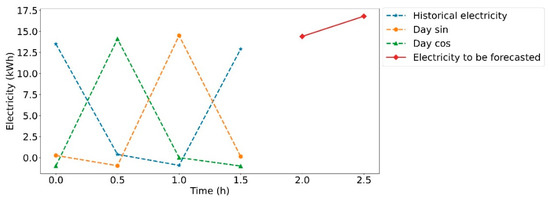
Figure 1.
A sample of the dataset predicting every half an hour in the following 1 h.
Day feature is converted to Day sin and Day cos, which, to some extent, can reflect the pattern of temperature variation, such as night-time is cooler than daytime. Machine Learning (ML) is adopted in this research to avoid complex calculations but maintain satisfying performance. The contributions of this study can be summarised in the following two points:
- The study confirms the model’s performance in the absence of weather features which makes the model less computational cost. It is almost effortless to deploy from an engineering prospect since no sensors for weather conditions are needed;
- The multi-output allows a detailed scenario to respond to the electricity usage in the following hours.
The remainder of the paper is organised as follows: Section 2 unveils the overview of the whole process from raw data collection and the development of ML models. Section 2 lays out data collection, analysis, and data pre-processing for ML models. Subsequently, details of three different ML algorithms, hyperparameter tuning, and evaluation criteria are discussed in the rest subsections of Section 2. Section 3 provides results for predicting the electricity usage in the next 30 min and discussions for a comparison with other research. Section 4 provides conclusions, limitations, and future directions.
2. Materials and Methods
2.1. Data Collection
The first step in predicting the electric energy consumption of a residential building is to collect energy consumption data. The selected building shall have a monitoring system that collects and monitors electricity consumption. The building studied is the University of Birmingham Chamberlain Halls of Residence. The residential halls of Chamberlain consist of four buildings, Linear Wing A, Linear Wing B, Linear Wing C, and the Tower. Linear Wing A to C is a 4-story construction, and the Tower is a 20-story construction. Chamberlain provides over 120 shared flats and studios. Optima Energy Systems manage chamberlain energy monitoring. After requesting the energy consumption data from the University of Birmingham, the university provided one year of electricity consumption data from December 2020 to December 2021. The temporal granularity of the data is half an hour.
Figure 2 uncovers the shape of the dataset showing that the dataset is slightly longer than one year, which exceeds a majority of studies ranging from two weeks to four years. However, this is not an appropriate justification for the dataset’s size. In [23], the authors well explained a common question arising when using ML—what is the proper size of data needed? The n–p ratio, where n refers to the number of samples and p stands for the number of features, is used to assess the data size. ML models are prone to overfitting when p is much larger than n. Therefore, more samples can be recruited to relieve or mitigate overfitting. The size of data is also sensitive to the complexity of algorithms, as a simple algorithm can present better performance than a complex algorithm when there is a limited number of samples [24]. There is no simple answer to the size of the dataset. However, it is sensible to ensure that the n is large enough to avoid overfitting and that the model can learn a representative pattern.
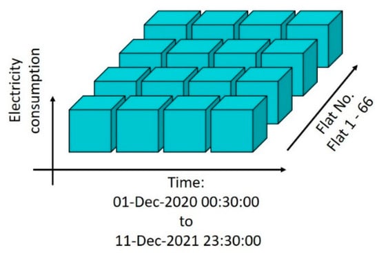
Figure 2.
Dimension of the dataset.
2.2. Exploratory Data Analysis
In this section, data analysis has been conducted to explore and summarise the main characteristics using an additive decomposition model and data visualisation methods. All the insights from this section underpin the ML model part. This section starts with a quick observation of the rolling mean and standard deviation (std), where a rolling window covering one day long is 48 slots, as seen in Figure 3. Several spikes in Figure 3a are considered to be outliers. Apart from the spikes, flat rolling mean and std with slight dip and rise can be found to reflect that the daily consumption is consistent over the year. To study the detail of the dataset, Figure 3b shows a seasonal pattern and pattern based on student timetable. There are three plateaus (after 1 December 2020, 15 March 2021, and 1 July 2020) responding to three breaks of the university and the mean value from 1 May 2021 to 1 July 2021 is lower than other months due to the higher temperature leading to no heating needed. The preliminary assessment infers that the trend in electricity consumption is time-related. It is noted that Figure 3c decomposes the first 2000 slots based on (1), yielding a seasonal trend. All these analyses have been performed to support the deployment of a time-series model since an explicit trend can be found and the rolling mean and std remains stable. To conquer the three plateaus, day features are also introduced.
where yt represents the data; St is the seasonal element; Tt is the trend; and Rt is the remainder component.
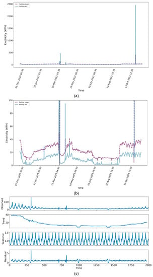
Figure 3.
Data mean and std: (a) the overall plotting, (b) zooming in plotting, and (c) seasonal decomposition by the additive model.
2.3. Data Preprocess
The data cover the electricity consumption for each flat on the selected date. It is not necessary to predict the trivial electricity consumption at the flat level so that the electric usage of each flat adds up to generate the consumption for the whole building according to dates and temporal granularities, as demonstrated in Figure 4.

Figure 4.
Electricity consumption of the whole building.
Outliers which enlarge the mean value and variance of the dataset can jeopardise models and result in biased parameter estimation, model misspecification, and wrong predictions. Therefore, it is necessary to identify them before model development. Boukerche et al. defined an outlier where a value diverges far from the main track [25], as seen in Figure 3a. The interquartile range (IQR) method is employed for the main appeal of IQR’s low sensitivity to distortion, as only the central part of the observation is desired [26]. Q1 (25 percentile) and Q3 (75 percentile) define the IQR, while the minimum and maximum values define where values inside the region are considered sensible. The outliers shown in Figure 5a are replaced by the maximum value defined in Figure 3.
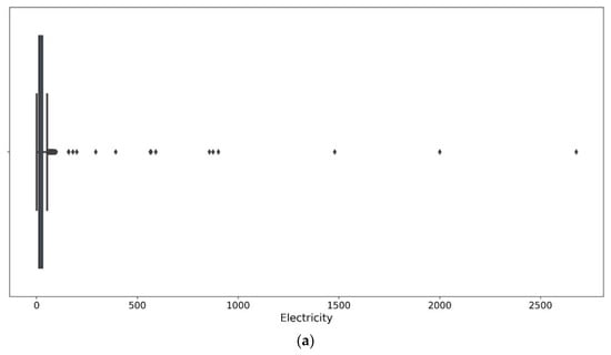
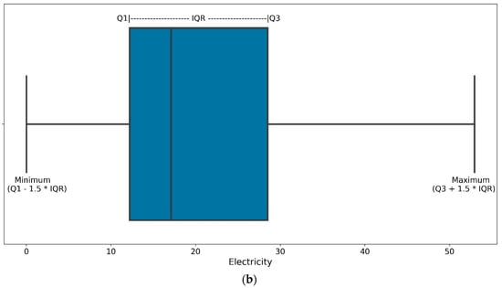
Figure 5.
Outlier processing: (a) before processing and (b) after processing.
The date and time attributes which need to be transformed are noted as they cannot be used by the AI model directly. To show the periodicity of the electricity usage, the date and time feature is converted to Day sin and Day cos using sine and cosine functions, as can be seen in Figure 6. After the above transformation, an example of the input and output can be seen in (2) and (3). It can be seen that (2) depicts an input with four timestamps and (3) provides an output with four timestamps. This means that the input features at the four historical timestamps are adopted to predict the electricity consumption at the future four timestamps. In this study, the number of input and predicted timestamps vary from 1 to 9 to evaluate the impact of the timestamps.
where E is electricity consumption; D is Day; subscript s and c stand for sine and cosine; and the superscript number is the number of timestamps.
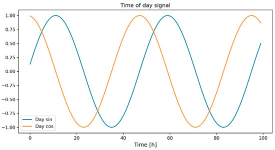
Figure 6.
Date and time transformation.
2.4. Machine Learning Models
Three powerful algorithms, Long Short-Term Memory (LSTM), XGBoost, and SVR, are provided for rigorous evaluation and to avoid potentially biased results.
LSTM, cut out for time-series problems, is famous for its cheap computational cost and high performance. Before Hochreiter et al. developed LSTM, recurrent backpropagation was haunted by the time-consuming issue when it tried to store information over extended time intervals, mainly due to insufficient decaying error backflow [27]. To eliminate this issue, LSTM, also known as the gradient-based method, truncated the gradient that will cause no harm and dedicated to linking up to 1000-time steps by making constant error flow to constant error carousels within special units. Multiplicative input and output gates were used to protect the constant error flow from irrelevant inputs and other units from unimportant memory contents [27].
XGBoost has gained success and has been booming in some competitions, such as Kaggle 2015 and KDDCup 2015. At Kaggle, 17 out of 29 winning teams utilised XGBoost, while a great success could also be seen at KDDCup 2015, which the top 10 teams all employed XGBoost [28]. From [29], the researchers have proposed four crucial factors that make XGBoost great success: highly scalable, a theoretically justified weighted quantile sketch for efficient proposal calculation, a new sparsity-award algorithm for parallel tree learning, and an effective cache-aware block for out-of-core tree learning. These techniques enable XGBoost to run ten times faster than common models on an individual machine.
SVR was proposed based on Vapnik’s concept in [30]. The core goal of SVR is to learn a target function with the most significant deviation from the actual targets for all training samples. Moreover, SVR is desperate for a flat function inferring that SVR is not sensitive to errors smaller than the deviation shown in Figure 7. However, the error outside the and is not tolerable.
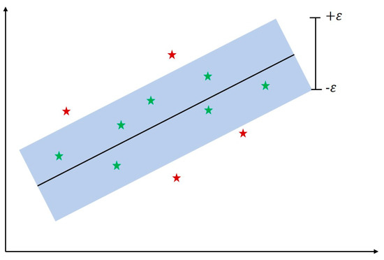
Figure 7.
SVR.
2.5. Hyper-Parameter Tuning
Manual search (MS) and grid search (GS) [31] are widely used to find the optimal hyperparameters of an ML model. MS is not that friendly for people fresh to ML as expertise and understanding of how the model works inside is required. Moreover, it is time-consuming to use MS and GS, while GS can also be a high computational cost if the search area is large. A more effective way, random search (RS), is required for model selection. Bergstra et al. have conducted a parametric analysis using a neural network configured with GS and RS under seven different datasets [32]. They concluded that RS outperforms GS with less computational time, and the performance of RS can be superior if the same computational budget is granted since RS can search in a larger space. Over four out of the seven datasets, the same performance was seen between RS and GS, but RS achieved one superior outcome. Another important finding from [32] is that only a limited amount of hyperparameters is sensitive to a dataset, but those critical hyperparameters vary with datasets. This reveals that if there is a requirement to re-train a model to work with a different dataset, GS is more difficult to use for a new dataset.
2.6. Metrics
Motivated by the growing importance and need for an energy forecasting system, the ASHRAE Great Energy Predictor Shootout leveraged and unified a metric, CV, to accurately compare the methods predicting hourly energy use based on building data [33]. Root Mean Squared Error (RMSE) [34], Mean Absolute Error (MAE) [35], and coefficient of determination (R2) [36,37] are also provided to allow in-depth insights into the results and benchmarking with other research as these metrics have also been widely used. The details of the three metrics are given as follows:
where is actual values; indicates predicted values; is the average value of the total energy consumption; and N is the number of samples. As seen in (4), a large numerator means an extensive error range leading to a high CV. It is noticeable that RMSE pays more attention to the error itself, while R2 focuses on a ratio of the error to actual and average values.
3. Results and Discussions
This section provides results based on the optimal models, which result from the random search method with the defined space in Table A2.
The best R2, RMSE, and CV for the different configurations due to the number of inputs and outputs for the 10% testing set (80% training set and 10% validation set) are in Table 1. In Table 1, the SVR provides the optimal performance by configuring one historical timestamp to predict the electricity consumption at the sequential timestamp. This capital scenario implies that the resident’s living pattern related to electricity usage is highly time-dependent as SVR can use the electricity consumption in this half an hour to predict that in the next half an hour well. Two out of three models in Table 1 depict comparable performance with 14% and 15% CV from the SVR and the XGBoost. The LSTM procures a slightly bigger CV than the other two. More insights regarding the number of inputs and outputs can be gained from Table A1. Table A1 lists how the SVR responds to the different number of inputs and outputs. It is apparent that the SVR is subjected to a large number of outputs showing less qualified to predict four or more outputs, especially using limited inputs. However, when three outputs are required, the SVR predictor can still at least promise 90% R2 and 19.801% CV.

Table 1.
Summary of the best result.
Table 2 displays some research in the same area to benchmark this study. They compete in terms of temporal granularity, building type, features, and data size. Compared to [38], which only focused on the cooling system, which relies on fewer features, this study investigates the electricity for the whole building, which can be affected by plenty of factors that make it hard to predict. CV provided by the SVR is slightly higher. However, the absence of weather features leads to no additional sensors being required. The same R2 can be seen from the SVR compared to [16], which also introduced seven weather conditions. It is noted that [16] aimed to predict hourly results, while the SVR model can predict in more detail two slots within one hour with 93% R2. The SVR performs better than [18], which implemented 140 sensors among the three residential buildings. The SVR uses fewer features compared to [22]. The 84-day dataset used in [22] is considered diminutive compared to the 1-year dataset used in this article. The SVR delivered a better CV of 14.25%, while [22] achieved a 14.88% CV for the sub-hourly prediction.

Table 2.
Comparative analysis of the result.
4. Conclusions
In this investigation, the aim is to develop a lightweight model to determine the future electricity consumption of a residential building based on historical information. This study has identified that even three features can work well with an elaborate tuning of an outstanding ML model SVR producing 14% CV. We broaden our investigation to evaluate the influence of the number of inputs and outputs, which has not been done before. Specifically, the time-series model, which depends more on the periodicity of the data, cannot improve itself by effortlessly adding the number of inputs which sometimes is a helpful tactic for the non-time series models. The finding that more output can impede the model’s performance will contribute to the area of multiple steps predictions.
To allow the practical implications for the proposed model, only a smart meter is required to monitor and record necessary features. This approach will provide flexible energy management to meet the net-zero goal and reduce CO2 emissions. A limitation of this study is that the building studied is a student accommodation which reflects high mobility each year due to graduation. Every academic year, many new students will move to the accommodation, resulting in slightly different electricity usage patterns. The model learnt from the previous year can give some biased predictions on the varied new pattern. Therefore, there is a potential that the model needs to be tuned regularly to ensure high performance. The performance of the proposed model for a new academic year can be guaranteed as the main feature of the building resulting from the university’s timetable will not change.
In future works, we will examine ensemble models [39], as the three models discussed here operate separately. There is a possibility that an ensemble method assembling several models in parallel or series can enhance robustness and generalizability over a single model.
Author Contributions
Conceptualisation: S.K., J.H. and M.A.; Investigation: S.K., J.H. and M.A.; Methodology: S.K., J.H. and M.A.; Data Analysis: J.H. and M.A.; Validation: J.H., and M.A.; Draft: J.H. and M.A.; Review and Editing: S.K. and J.H. All authors have read and agreed to the published version of the manuscript.
Funding
This research was funded by H2020 MSCA, grant number 691135. The APC was funded by MDPI’s Invited Paper Initiative.
Institutional Review Board Statement
Not applicable.
Informed Consent Statement
Not applicable.
Data Availability Statement
Data can be made available upon request for collaboration.
Acknowledgments
The authors are sincerely grateful to European Commission for the financial sponsorship of the H2020-MSCA-RISE Project No. 691135 "RISEN: Rail Infrastructure Systems Engineering Network," which enables a global research network that tackles the grand challenge of railway infrastructure resilience and advanced sensing in extreme environments (www.risen2rail.eu (accessed on 26 September 2022)) (Kaewunruen et al., 2016). The authors are grateful to the University of Birmingham’s Estates Department for the technical assistance of data collection and building physics model. The APC has been sponsored by MDPI’s Invited Paper Initiative.
Conflicts of Interest
The authors declare no conflict of interest.
Appendix A

Table A1.
Comparative analysis of the result.
Table A1.
Comparative analysis of the result.
| The no. of Inputs | The no. of Outputs | Testing R2 | RMSE | CV (%) | MAE |
|---|---|---|---|---|---|
| 1 | 1 | 0.953518 | 2.620952 | 14.25236 | 1.700528 |
| 2 | 1 | 0.951107 | 2.691193 | 14.66036 | 1.760021 |
| 4 | 1 | 0.949834 | 2.732484 | 14.87774 | 1.809715 |
| 3 | 1 | 0.948978 | 2.752481 | 14.99133 | 1.793756 |
| 9 | 1 | 0.948214 | 2.789799 | 15.24027 | 1.836671 |
| 8 | 1 | 0.947892 | 2.796634 | 15.26033 | 1.859448 |
| 7 | 1 | 0.947191 | 2.812954 | 15.33542 | 1.843559 |
| 5 | 1 | 0.945543 | 2.850398 | 15.52231 | 1.84593 |
| 6 | 1 | 0.944791 | 2.873362 | 15.65309 | 1.864009 |
| 1 | 2 | 0.928819 | 3.245625 | 17.69942 | 2.078487 |
| 9 | 2 | 0.929776 | 3.249956 | 17.77945 | 2.12982 |
| 8 | 2 | 0.928676 | 3.272915 | 17.88575 | 2.147037 |
| 2 | 2 | 0.926786 | 3.295525 | 17.9669 | 2.120674 |
| 4 | 2 | 0.92628 | 3.314742 | 18.0658 | 2.15817 |
| 7 | 2 | 0.926563 | 3.318645 | 18.11707 | 2.146832 |
| 3 | 2 | 0.924467 | 3.351245 | 18.26608 | 2.153108 |
| 6 | 2 | 0.923579 | 3.382362 | 18.44958 | 2.180407 |
| 5 | 2 | 0.922765 | 3.396789 | 18.51793 | 2.178441 |
| 8 | 3 | 0.912832 | 3.618912 | 19.80815 | 2.382346 |
| 9 | 3 | 0.91182 | 3.643122 | 19.95959 | 2.387658 |
| 7 | 3 | 0.908606 | 3.702905 | 20.24705 | 2.397612 |
| 1 | 3 | 0.90163 | 3.817739 | 20.83863 | 2.398218 |
| 6 | 3 | 0.902258 | 3.826442 | 20.90294 | 2.456909 |
| 2 | 3 | 0.900004 | 3.853622 | 21.02873 | 2.444086 |
| 4 | 3 | 0.899262 | 3.877127 | 21.15628 | 2.470191 |
| 5 | 3 | 0.899529 | 3.8759 | 21.15871 | 2.484479 |
| 3 | 3 | 0.898187 | 3.893086 | 21.24173 | 2.465941 |
| 1 | 4 | 0.873442 | 4.332329 | 23.67179 | 2.704412 |
| 2 | 4 | 0.869945 | 4.397046 | 24.02154 | 2.760474 |
| 1 | 5 | 0.843701 | 4.815976 | 26.34899 | 2.989854 |
| 2 | 5 | 0.839289 | 4.889294 | 26.74877 | 3.036636 |
| 1 | 6 | 0.817151 | 5.20917 | 28.54327 | 3.232244 |
| 1 | 7 | 0.794325 | 5.523127 | 30.31602 | 3.44357 |
| 1 | 8 | 0.776903 | 5.747819 | 31.61279 | 3.621202 |
| 1 | 9 | 0.76303 | 5.915412 | 32.61033 | 3.764738 |

Table A2.
Optimal hyperparameters for the three algorithms.
Table A2.
Optimal hyperparameters for the three algorithms.
| Algorithms | Hyperparameters | Searching Space | Optimal Value |
|---|---|---|---|
| LSTM | The no. of LSTM layers | 1–8 | 4 |
| The no. of units for LSTM layer 1 | 32–256 | 128 | |
| The no. of units for LSTM layer 2 | 32–256 | 64 | |
| The no. of units for LSTM layer 3 | 32–256 | 64 | |
| The no. of units for LSTM layer 4 | 32–256 | 192 | |
| The no. of dense layers | 1–8 | 3 | |
| The no. of units for dense layer 1 | 32–256 | 89 | |
| The no. of units for dense layer 2 | 32–256 | 40 | |
| The no. of units for dense layer 3 | 32–256 | 73 | |
| Learning rate | 1 × 10⁻¹–1 × 10⁻⁶ | 0.001347157 | |
| XGBoost | subsample | 1 × 10⁻³–5 × 10⁻¹ | 0.1 |
| No. of estimators | 1–2000 | 60 | |
| Min samples split | 2–50 | 0.1 | |
| Max depth | 2–50 | 5 | |
| Learning rate | 0.1–0.9 | 0.1 | |
| eta | 1 × 10⁻³–5 × 10⁻¹ | 0.8 | |
| Colsample bytree | 1 × 10⁻³–5 × 10⁻¹ | 0.8 | |
| SVR | Epsilon | 1 × 10⁻²–2 × 10⁻¹ | 0.16 |
| C | 1–2000 | 943 | |
| Kernel | rbf | rbf |
References
- GBC, U. UKGBC’s Vision for a Sustainable Built Environment Is One That Mitigates and Adapts to Climate Change. 2022. Available online: https://www.ukgbc.org/climate-change-2/ (accessed on 8 August 2022).
- Evans, S. Analysis: UK’s CO2 Emissions Have Fallen 29% over the Past Decade. 2020. Available online: https://www.carbonbrief.org/analysis-uks-co2-emissions-have-fallen-29-per-cent-over-the-past-decade/ (accessed on 8 August 2022).
- Langevin, J.; Harris, C.B.; Reyna, J.L. Assessing the potential to reduce US building CO2 emissions 80% by 2050. Joule 2019, 3, 2403–2424. [Google Scholar] [CrossRef]
- Singh, S.; Yassine, A. Big data mining of energy time series for behavioral analytics and energy consumption forecasting. Energies 2018, 11, 452. [Google Scholar] [CrossRef]
- Amasyali, K.; El-Gohary, N.M. A review of data-driven building energy consumption prediction studies. Renew. Sustain. Energy Rev. 2018, 81, 1192–1205. [Google Scholar] [CrossRef]
- Zhao, H.-X.; Magoulès, F. A review on the prediction of building energy consumption. Renew. Sustain. Energy Rev. 2012, 16, 3586–3592. [Google Scholar] [CrossRef]
- Clarke, J.A. Energy Simulation in Building Design; Routledge: London, UK, 2007. [Google Scholar]
- McQuiston, F.C.; Parker, J.D.; Spitler, J.D. Heating, Ventilating, and Air Conditioning: Analysis and Design; John Wiley & Sons: Hoboken, NJ, USA, 2004. [Google Scholar]
- ISO EN 13790:2008; Energy Performance of Buildings—Calculation of Energy Use for Space Heating and Cooling. International Organization for Standardization: Milan, Italy, 2008.
- Tealab, A. Time series forecasting using artificial neural networks methodologies: A systematic review. Future Comput. Inform. J. 2018, 3, 334–340. [Google Scholar] [CrossRef]
- Pisner, D.A.; Schnyer, D.M. Support vector machine. In Machine Learning; Elsevier: Amsterdam, The Netherlands, 2020; pp. 101–121. [Google Scholar]
- Peng, L.; Wang, L.; Xia, D.; Gao, Q. Effective energy consumption forecasting using empirical wavelet transform and long short-term memory. Energy 2022, 238, 121756. [Google Scholar] [CrossRef]
- Jin, N.; Yang, F.; Mo, Y.; Zeng, Y.; Zhou, X.; Yan, K.; Ma, X. Highly accurate energy consumption forecasting model based on parallel LSTM neural networks. Adv. Eng. Inform. 2022, 51, 101442. [Google Scholar] [CrossRef]
- Shahani, N.M.; Zheng, X.; Liu, C.; Hassan, F.U.; Li, P. Developing an XGBoost Regression Model for Predicting Young’s Modulus of Intact Sedimentary Rocks for the Stability of Surface and Subsurface Structures. Front. Earth Sci 2021, 9, 761990. [Google Scholar] [CrossRef]
- Ciulla, G.; D’Amico, A. Building energy performance forecasting: A multiple linear regression approach. Appl. Energy 2019, 253, 113500. [Google Scholar] [CrossRef]
- Solomon, D.M.; Winter, R.L.; Boulanger, A.G.; Anderson, R.N.; Wu, L.L. Forecasting Energy Demand in Large Commercial Buildings Using Support Vector Machine Regression; Department of Computer Science, Columbia University: New York, NY, USA, 2011. [Google Scholar]
- Edwards, R.E.; New, J.; Parker, L.E. Predicting future hourly residential electrical consumption: A machine learning case study. Energy Build. 2012, 49, 591–603. [Google Scholar] [CrossRef]
- Qiong, L.; Peng, R.; Qinglin, M. Prediction model of annual energy consumption of residential buildings. In Proceedings of the 2010 International Conference on Advances in Energy Engineering, Beijing, China, 19–20 June 2010; pp. 223–226. [Google Scholar]
- Hawkins, D.; Hong, S.M.; Raslan, R.; Mumovic, D.; Hanna, S. Determinants of energy use in UK higher education buildings using statistical and artificial neural network methods. Int. J. Sustain. Built Environ. 2012, 1, 50–63. [Google Scholar] [CrossRef]
- Leung, M.C.; Tse, N.C.F.; Lai, L.L.; Chow, T.T. The use of occupancy space electrical power demand in building cooling load prediction. Energy Build. 2012, 55, 151–163. [Google Scholar] [CrossRef]
- Platon, R.; Dehkordi, V.R.; Martel, J. Hourly prediction of a building’s electricity consumption using case-based reasoning, artificial neural networks and principal component analysis. Energy Build. 2015, 92, 10–18. [Google Scholar] [CrossRef]
- Jain, R.; Damoulas, T.; Kontokosta, C. Towards data-driven energy consumption forecasting of multi-family residential buildings: Feature selection via the lasso. In Computing in Civil and Building Engineering; ASCE: Alexander, AL, USA, 2014; pp. 1675–1682. [Google Scholar]
- Bzdok, D.; Krzywinski, M.; Altman, N. Points of Significance: Machine learning: A primer. Nat Methods 2017, 14, 1119–1120. [Google Scholar] [CrossRef] [PubMed]
- Jordan, M.I.; Mitchell, T.M. Machine learning: Trends, perspectives, and prospects. Science 2015, 349, 255–260. [Google Scholar] [CrossRef]
- Boukerche, A.; Zheng, L.; Alfandi, O. Outlier detection: Methods, models, and classification. ACM Comput. Surv. CSUR 2020, 53, 1–37. [Google Scholar] [CrossRef]
- Vinutha, H.; Poornima, B.; Sagar, B. Detection of outliers using interquartile range technique from intrusion dataset. In Information and Decision Sciences; Springer: Berlin/Heidelberg, Germany, 2018; pp. 511–518. [Google Scholar]
- Hochreiter, S.; Schmidhuber, J. Long Short-Term Memory. Neural Comput. 1997, 9, 1735–1780. [Google Scholar] [CrossRef]
- Bennett, J.; Lanning, S. The netflix prize. In Proceedings of the KDD Cup and Workshop 2007, San Jose, CA, USA, 12 August 2007; p. 35. [Google Scholar]
- Chen, T.; Guestrin, C. Xgboost: A scalable tree boosting system. In Proceedings of the 22nd Acm Sigkdd International Conference on Knowledge Discovery and Data Mining, San Francisco, CA, USA, 13–17 August 2016; pp. 785–794. [Google Scholar]
- Cortes, C.; Vapnik, V. Support-vector networks. Mach. Learn. 1995, 20, 273–297. [Google Scholar] [CrossRef]
- Liashchynskyi, P.; Liashchynskyi, P. Grid search, random search, genetic algorithm: A big comparison for NAS. arXiv 2019, arXiv:1912.06059. [Google Scholar]
- Bergstra, J.; Bengio, Y. Random search for hyper-parameter optimization. J. Mach. Learn. Res. 2012, 13, 281–305. [Google Scholar]
- Kreider, J.F.; Haberl, J.S. Predicting hourly building energy use: The great energy predictor shootout—Overview and discussion of results. In Proceedings of the 1994 American Society of Heating, Refrigerating, and Air Conditioning Engineers (ASHRAE) Annual Meeting, Orlando, FL, USA, 25–29 June 1994. [Google Scholar]
- Chai, T.; Draxler, R.R. Root mean square error (RMSE) or mean absolute error (MAE)?–Arguments against avoiding RMSE in the literature. Geosci. Model Dev. 2014, 7, 1247–1250. [Google Scholar] [CrossRef]
- Karunasingha, D.S.K. Root mean square error or mean absolute error? Use their ratio as well. Inf. Sci. 2022, 585, 609–629. [Google Scholar] [CrossRef]
- Piepho, H.P. A coefficient of determination (R2) for generalized linear mixed models. Biom. J. 2019, 61, 860–872. [Google Scholar] [CrossRef] [PubMed]
- Chicco, D.; Warrens, M.J.; Jurman, G. The coefficient of determination R-squared is more informative than SMAPE, MAE, MAPE, MSE and RMSE in regression analysis evaluation. PeerJ Comput. Sci. 2021, 7, e623. [Google Scholar] [CrossRef] [PubMed]
- Wang, J.Q.; Du, Y.; Wang, J. LSTM based long-term energy consumption prediction with periodicity. Energy 2020, 197, 117197. [Google Scholar] [CrossRef]
- Sideratos, G.; Ikonomopoulos, A.; Hatziargyriou, N.D. A novel fuzzy-based ensemble model for load forecasting using hybrid deep neural networks. Electr. Power Syst. Res. 2020, 178, 106025. [Google Scholar] [CrossRef]
Publisher’s Note: MDPI stays neutral with regard to jurisdictional claims in published maps and institutional affiliations. |
© 2022 by the authors. Licensee MDPI, Basel, Switzerland. This article is an open access article distributed under the terms and conditions of the Creative Commons Attribution (CC BY) license (https://creativecommons.org/licenses/by/4.0/).