A Seismic Phase Recognition Algorithm Based on Time Convolution Networks

Abstract

Over recent years, frequent earthquakes have caused huge losses in human life and property. Rapid and automatic earthquake detection plays an important role in earthquake warning systems and earthquake operation mechanism research. Temporal convolution networks (TCNs) are frameworks that use expansion convolution and expansion, which have large and temporal receptive fields and can adapt to time series data. Given the excellent performance of temporal convolution networks using time series data, this paper proposes a deep learning framework based on the temporal convolution network model, which can be used to detect and obtain the accurate start times of seismic phases. In addition, a convolutional neural network (CNN) was added to the temporal convolution network model to automatically extract the deep features of seismic waves and the expansion convolution of each level was added to optimize its structure, which not only reduced the experimental parameters but also produced high-precision seismic phase detection results. Finally, the model was compared to the TCN, CNN-LSTM, SELD-TCN and the traditional AR-AIC methods. Our experimental results showed that the S-TCN method demonstrated great advantages in the accuracy and performance of seismic phase detection.

1. Introduction

At present, artificial intelligence (AI) methods are widely used within the field of geophysical research and have achieved great results using deep neural networks. AI can be used to process massive amounts of seismic data by improving deep network generalization to provide more effective data for the inversion of the geological structures in existing seismic catalogs. Due to the improvements in seismic observation methods over recent years, the rapid and high-precision automatic detection of seismic data has become the focus of research.

Over recent years, deep learning has also developed rapidly and more and more seismologists have begun to use deep neural networks to obtain information from seismic data, such as seismic phase identification, earthquake location detection, seismic phase mechanism solutions, aftershock searches, earthquake early warning systems and forecasts. Yu et al. (2018) trained a 17-layer inception deep network model to detect the start times of near-seismic P and S wave phases [1] (P and S waves are two kinds of seismic waves: P waves are longitudinal waves, i.e., vertical shaking, and S waves are transverse waves, i.e., horizontal shaking; P waves are also faster than S waves). During the training process, the authors considered the addition of noise to the label data, the regularization of the output results from the convolutional layers, the dropout operation and training methods based on noise stepping, which improved the generalization ability of their neural network. This method could directly output the start time of a seismic phase with better stability than the traditional method and it could adapt to seismic signals with different signal-to-noise ratios. Ross et al. (2018) trained a convolutional neural network (CNN) classifier using more than 4.8 million seismograms from Southern California, USA, that were manually labeled with P wave start times and polarities and achieved the automated high-precision measurement of P wave start times and initial motion polarities [2]. Since the network structures of CNN convolution and filtering effectively learn features directly from data, thereby avoiding model construction and other tasks, deep neural networks can achieve great results in seismic phase detection research. Zhu et al. (2019) used U-Net and probability distribution methods to automatically detect earthquake phases in Southern California for the first time, which provided a novel way for image segmentation structures to detect earthquake phases [3] and achieved good results. On this basis, Zhao et al. (2019) redesigned a U-shaped network algorithm to create the Unet_cea structure. They used more than 80,000 seismic data points from earthquakes of different magnitudes and signal-to-noise ratios that were recorded during Wenchuan aftershocks and from the Metropolitan Seismic Network for training and testing. During their testing, the automatic identification and timely detection of seismic phases were realized and a high level of accuracy was also obtained [4]. The U-shaped network had a significantly higher hit rate and a lower root mean square error than the STA/LTA and kurtosis analysis automatic detection methods.

With the development of deep neural networks, forming fusion structures using different structures has gradually become the new trend. Zhou et al. (2019) designed a CNN and recurrent convolutional network tandem structure to detect P and S waves in continuous seismic waveforms [5]. They used an eight-layer CNN to distinguish between seismic signals and noise data and then input a two-layer bidirectional recurrent neural network (RNN) structure to extract the start times of the P and S waves. Their results showed that this method could achieve an extremely small error rate and high accuracy. Liu et al. (2020) designed an improved U-Net model that could use AI to capture competition and Hi-net data training, which achieved accurate time extraction from continuous waveforms [6].

Li et al. (2020) designed a joint loss function for classification and regression and demonstrated the excellent performance of deep neural networks in seismic phase detection by building a multitask convolutional neural network model [7]. Yu et al. (2020) introduced a cascaded classification and regression framework for seismic phase detection, named the classification and regression phase net (CRPN), which contained two convolutional neural network models with different complexities to meet the accuracy and efficiency requirements [8]. Guo et al. (2022) revealed the spatial and temporal distribution characteristics of earthquake sequences and the geometry of seismogenic faults by building a high-resolution earthquake catalog [9]. Liao et al. (2021) processed continuous seismic waveform data and dense seismic sequences in real time and offline by designing a real-time seismic processing system based on artificial intelligence. Scientific research provided important technical support [10].

Recent findings have shown that temporal convolution networks (TCNs) [11,12] outperform baseline recurrent architectures in a wide range of sequence modeling tasks, including action segmentation [13], speech analysis and synthesis tasks [11,14]. The research results that were published by Yan et al. (2020) [15] on the use of TCNs for weather forecasting tasks showed that TCNs performed well in prediction tasks using time series data. Guirguis et al. (2020) [16] proposed an SELD-TCN architecture based on the sound event localization and detection (SELD) and TCN methods. By applying a short-time Fourier transform, the SELD-TCN method could extract the phases and magnitudes of the spectrum and stack them as separate input features, then connect the convolutional and recurrent blocks (bidirectional GRUs) and finally connect the fully connected blocks. The outputs of SELD-Net were sound event detection (SED) and the direction of arrival (DOA). Since the dilated convolutions enabled the network to handle a variety of inputs, deeper networks (which suffer from unstable gradients during backpropagation) could be required. The authors overcame this challenge by adopting a WaveNet [17]. They showed that SELD tasks did not require a recurrent layer and they successfully detected the start and end times of active sound events. Since earthquake phases are sets of time-correlated time series data, TCNs not only achieve a better performance but also reduce the computational costs of training compared to RNNs and their variants, without exploiting repetitive architectures.

In view of the above analysis, this paper proposes an S-TCN model based on temporal convolutional neural networks, which could improve the model by using dilated convolutions and dilation frameworks. We also added a convolution module to extract the deep features of seismic waves to obtain accurate seismic phase detection and provide new ideas for earthquake early warning systems.

2. Data

2.1. Dataset

Since the quality of datasets directly affects the results of network training, this study used the Global Seismic Signals Dataset (STEAD) [18], which was provided by the Seismological Laboratory of Stanford University, to ensure that there were sufficient training data and to ensure the generalization of the network structure. Most of the seismic records in this dataset were recorded in the United States and Europe. The STEAD dataset includes two categories of seismic and non-seismic signals, which were recorded using seismic instruments with 2613 receivers (seismographs) worldwide, as shown in Figure 1. These receivers were located at local distances, i.e., within 350 km of the earthquakes. The non-seismic category currently only contains one subcategory (seismic noise), which includes about 100,000 samples. The locations of the instruments that recorded the noise waveforms are shown in Figure 2.

Figure 3 shows the magnitude distribution of the recorded earthquakes. Small earthquakes (less than magnitude 2.5) make up the majority of the dataset. All seismic data have three components: the vertical, east–west and north–south directions. The sampling rate of the data is 100 Hz and the length of the seismic data is 60 s. Each data window contains longitudinal and shear waves, from the longitudinal waves (P waves) that occur 5–10 s before the start of the earthquakes to at least 5 s after the arrival of the shear waves (S waves). Additionally, all waveforms were detrended, de-averaged and band-pass filtered.

We selected a total of 100,000 data points from the STEAD dataset. We then processed the data are as follows:

(1) The waveforms were cut according to the first arrival sampling points of the P waves and the first arrival sampling points of the S waves, which were provided by the data tags. First, they were cut 3–5 s before the arrival of the P waves as the starting points of the waveforms and 10 s after the arrival of the S waves as the end points of the waveforms, then they were cut it into waveform data with a length of 30 s. When the length after cropping was less than 30 s, the data were randomly supplemented with zero values before and after the cropped data. Then, the data were cut from 60 s to 30 s, with a sampling rate of 100 Hz and a segment length of 3000. We filtered the 30 s data to ensure that they contained the arrival points of the P and S waves, which left us with 97132 data points.

(2) We then evenly distributed the P waves over intervals of 200–600 by performing translation processing on the data. The distributions of the data before and after processing are shown in Figure 4. After processing, a min–max normalization was performed, which left us with 65,000 data points. Then, we randomly scrambled the data.

(3) Next, we divided the processed dataset to obtain a training set with 52,000 data points, a validation set with 6500 data points and a testing set with 6500 data points (8:1:1).

(4) Since the network output length was 371 when one-hot processing was performed on the labels, the labels were processed as one-hot labels with a length of 371. The labeling positions comprised 40 time steps before and after the manual labeling, with a one-hot label length of 11. The original data and the labeled data that corresponded to the labels are shown in Figure 5.

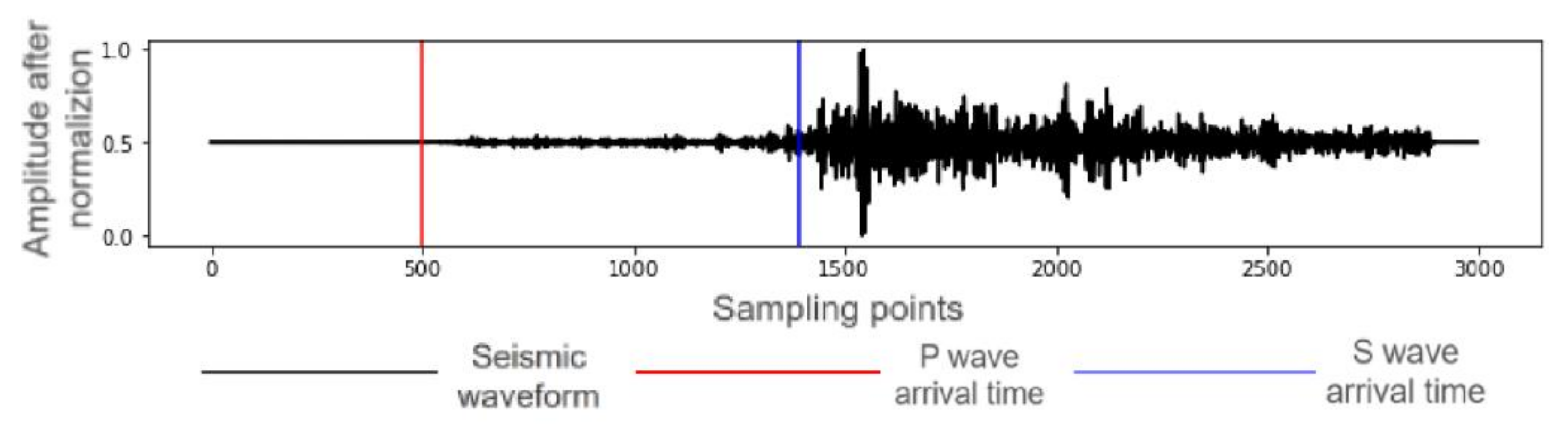
2.2. Data Preprocessing

Data preprocessing is of great significance in the training of neural networks as preprocessing processes directly affect the model convergence effect. The original data in this study comprised continuous waveform segments with a time window length of 30 s and a data frequency of 100 Hz, so the data format was a two-dimensional matrix of 3000 × 3. Due to the existence of low-frequency long-term background disturbances and high-frequency noise in the waveform data, our model received too many useless signal features during the training process, which reduced the fitting effect. Therefore, the band-pass filtering method was first performed during the data processing on [0.1, 20] of the original data. A continuous wavelet transform was then used to decompose the signals into components at different scales [19,20,21,22]. Finally, the amplitude differences between the time steps in the seismic data were too large, so to reduce the variations in the data and make the convergence process of the loss function smoother, it was necessary to normalize each component of the waveform data using the following calculation formula:

$$A_i=\frac{A_i}{max\left(\left|A_i\right|\right)}$$

(1)

where A${}_i$ is the amplitude of the i-th sampling point in each track component. An example original waveform is shown in Figure 6, where the red vertical line represents the arrival time of the P wave and the blue vertical line represents the arrival of the S wave (which were manually marked by seismological researchers).

3. Neural Network Structure

In this section, we introduce our improved seismic phase detection model (S-TCN), which was based on traditional TCNs. The specific parts of our model are discussed in the following subsections: the first subsection introduces the traditional time-domain convolutional network principle and the second subsection introduces the improved S-TCN model.

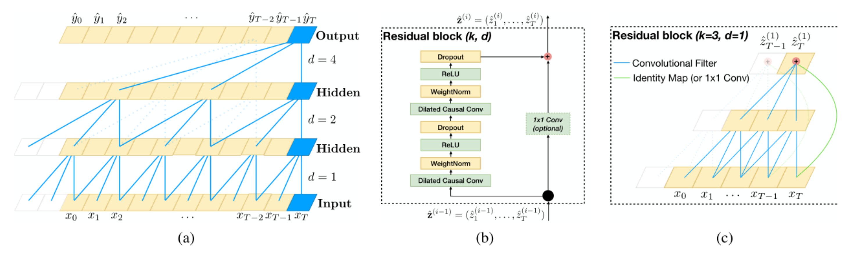
3.1. Temporal Convolutional Network

Traditional time series neural networks, such as RNNs, long short-term memory (LSTM) and other models, have certain problems, such as being time-consuming, poor parallelism and long-term dependencies. However, TCNs can solve these problems. TCNs, which is short for temporal convolutional networks, consist of dilated and causal 1D convolutional layers that have the same input and output lengths.

The design of TCNs is based on two principles: (1) the input and output of the network are the same length; (2) there is no “leakage” of past information. To achieve the same input length, TCNs use 1D fully convolutional networks (1D FCNs), in which each hidden layer is the same length as the input layer. Then, zero-padding (kernel size 1) is added to ensure that all of the layers have the same length. To achieve the same output length, TCNs use causal convolution, in which the output at time t is only convolved with earlier elements from time t and the previous layer. In a nutshell, TCNs = 1D FCNs + causal convolution. Dilated convolution is also used in TCNs. The advantage of using dilated convolution is an increase in the receptive fields without a loss of information in the pooling operations, so each convolution output contains a large range of information. The structure of a generic TCN is shown in Figure 7.

By analyzing Figure 7, it can be seen that TCNs utilize the 1D FCN structure and that TCNs have a stronger ability to retain long-term historical information than LSTM. To maintain the same time step, the input and output of each hidden layer have the same length. Specifically, in the first hidden layer, when the input is n time steps, then the output is also n time steps, regardless of the kernel size and dilation. Similarly, the input and output time steps of other hidden layers are all n, which is very similar to the structure in RNNs. No matter the layer, the input of each time step has a corresponding output.

TCNs use causal convolution. Causal convolution for the output data at time t means that the input can be t or the time before t. This structure is shown in Figure 8. For filter F = (f${}_1$, f${}_2$, …, f${}_K$) and sequence X = (x${}_1$, x${}_2$, …, x${}_T$), the causal convolution at x${}_t$ is defined as:

$$(F\ast X)\left(x_t\right)={\sum }_{k=1}^K{f}_k{x}_{(t-K+k)}$$

(2)

For filter F = (f${}_1$, f${}_2$, …, f${}_K$) and sequence X = (x${}_1$, x${}_2$, …, x${}_T$), the dilated convolution at x${}_t$ with a dilation factor d is defined as:

$$(F\ast dX)\left(x_t\right)={\sum }_{k=1}^K{f}_k{x}_{(t-(K-k\left)d\right)}$$

(3)

Dilated convolution enables networks to process various inputs, so deeper networks are required. To solve the problem of deeper networks potentially causing gradient disappearance, dilated convolution uses a difference block structure, similar to the structure in ResNet [23], through which TCNs can gain a higher generalization ability. As shown in Figure 7c, the residual structure replaces the simple connections between the TCN layers. Since the number of channels in x and F(x) is different, a 1 × 1 Conv has been designed to enable a simple transformation of x, so that the transformed x and F(x) can be added.

3.2. Improved S-TCN Structure Based on TCNs

Our S-TCN model mainly included four modules (the structure is shown in Figure 9):

(a) Input representation: seismic waves that were sampled at 100 Hz were input into the network after data preprocessing using the linear band-pass filtering (continuous wavelet transform) normalization step;

(b) Convolution block: to learn the inter- and intra-channel features, three consecutive 1D convolution blocks were input into the model. The size of the convolution kernel was set to 6*1 and the number of convolution kernels was set to 16, 32 or 64 to extract features at different scales. In addition, the output was batch normalized and the rectified linear unit (ReLU) activation function was used. The block dropout operation was used in the last convolution block;

(c) TCN block: to learn the contextual information of the seismic phases, the output of the convolution block was reshaped into 1D and then sent to three consecutive TCN blocks. The TCN blocks could utilize the full context of the input sequence;

(d) Time distributed module: the output of the TCN blocks was fed into two parallel branches of the time distributed module, each of which consisted of its own time distributed module, which performed the final phase identification and detection.

Figure 9. A network structure diagram of our S-TCN model.

Figure 9. A network structure diagram of our S-TCN model.

Unlike neuron networks, which attempt to learn the underlying structures in sequences using dilated convolution, non-neuron networks can handle a wider range of inputs. In general, when d = 1, normal convolution is performed. On the other hand, the higher the inflation factor, the larger the receptive field, so the kernels expand over a more comprehensive input area. To obtain such a large exponential receptive field for TCNs, deeper networks are required, which suffer from unstable gradients during backpropagation. To overcome this limitation, residual connections are used to learn the modifications to the identity maps. Generally, TCNs utilize causal convolution, in which the output at time t depends on current and past elements. This step can be achieved using zero-padding. However, in this study, convolution within the TCN blocks was modified to be non-causal, with batch normalization employed immediately after dilated convolution to mimic the use of future knowledge by bidirectional neural networks. Next, the normalized output was passed to the ReLU function for activation. Finally, a dropout function with a loss rate of 0.5 was used for correction.

4. Experiments

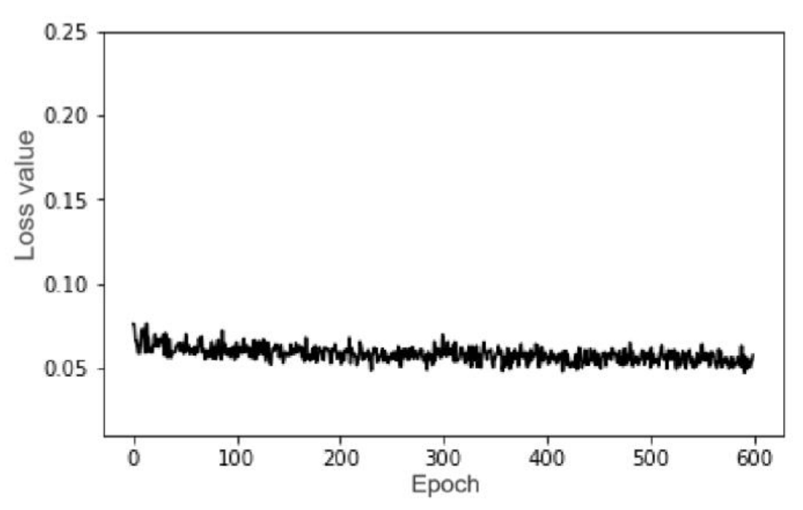
4.1. Training Process

In our experiments, we used the Tensorflow framework to train the network. The loss function used binary_crossentropy. The initial learning rate was 0.01 and was set to decay. The adaptive moment estimate (ADAM) algorithm was used for optimization [24].

Once 20 consecutive epochs did not drop, the loss function training stopped with a total of trained 302 epochs. A loss function graph of the training set is shown in Figure 10 and a loss graph of the testing set is shown in Figure 11.

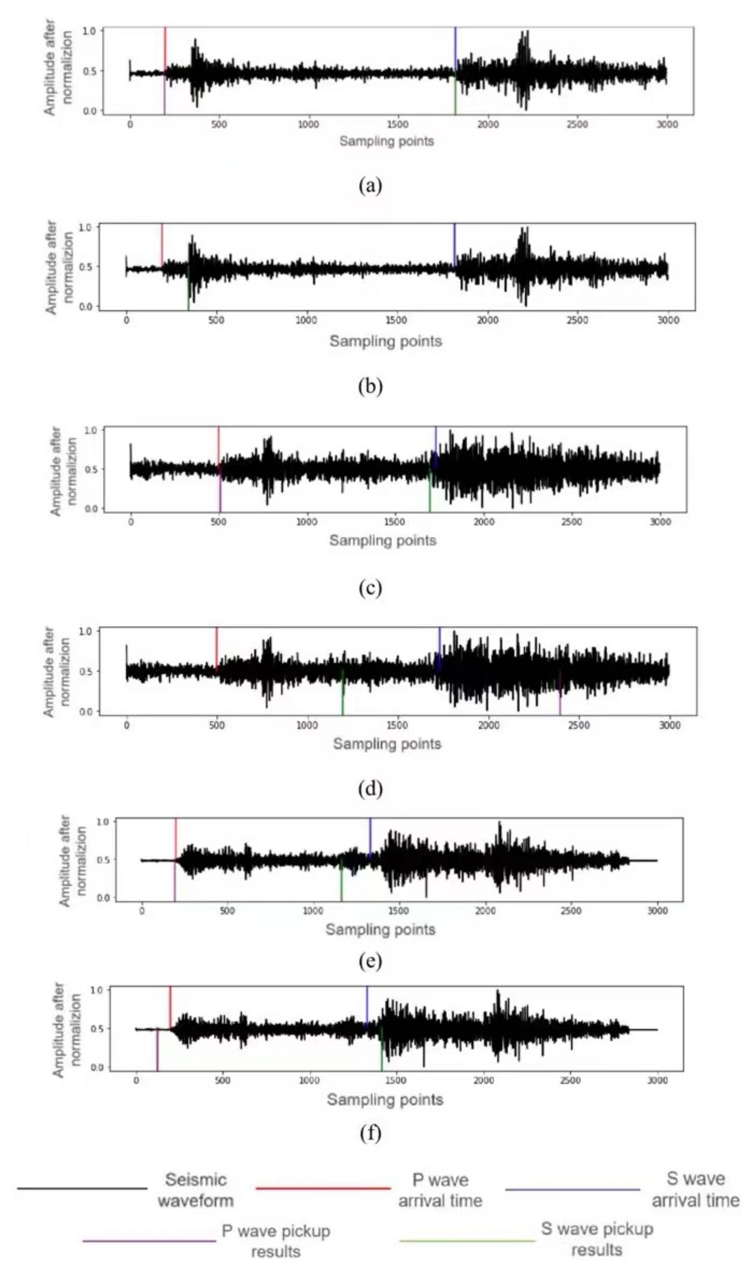
4.2. Evaluation Standards

The mean error refers to the arithmetic mean of the random errors from all values that have been measured using measurements of equal precision. It is a measure of the expected value of the square of the difference between the parameter estimate and the true value of the parameter. The calculation formula is as follows:

$$\eta =\frac{1}{n}{\sum }_{i=1}^n\left|x_i-\overline{x}\right|$$

(4)

The mean errors can also be identified manually using the following error calculation formula:

$$Error=\left||Modelpredictedtime-Manualmeasuringtime\right||$$

(5)

From

Table 1. A comparison of the detection of P and S waves between the TCN and the SELD-TCN models.

Model	P Wave Detection			S Wave Detection
	Average Error	Error within 0.2 s	Error within 0.5 s	Average Error	Error within 0.2 s	Error within 0.5 s
TCN	1.25 s	75%	81.90%	4.01 s	17.30%	29.80%
SELD-TCN-1	0.29 s	57.50%	96.20%	0.84 s	46.10%	79.20%
SELD-TCN-2	0.34 s	74.40%	94.60%	0.91 s	50.30%	76.9%

and

Table 2. A comparison of errors in the detection of P and S waves between the TCN and the SELD-TCN models.

Model	Dataset	P Wave Detection			S Wave Detection
		Average Error	Error within 0.2 s	Error within 0.5 s	Average Error	Error within 0.2 s	Error within 0.5 s
TCN	Training	2.257 s	56.94%	64.95%	6.029 s	6.75%	13.26%
	Testing	1.844 s	63.13%	72.07%	5.699 s	5.03%	12.85%
S-TCN	Training	0.266 s	70.01%	86.01%	1.089 s	49.08%	76.25%
	Testing	0.204s	69.27%	97.76%	1.866 s	50.84%	74.86%
AR-AIC	Testing	1.269 s	60.39%	73.82%	1.498 s	56.61%	68.49%

, it can be seen that the average error of S-TCN was smaller than that of the traditional TCN. On the testing set and for the arrival of P waves, the proportion of S-TCN results with errors that were less than 0.2 s was 69.27%, which was higher than that of the TCN (63.13%), and the proportion of S-TCN results with errors that were less than 0.5 s was 97.76%, which was also higher than that of the TCN (72.07%). For the arrival of S waves, the proportion of S-TCN results with errors that were less than 0.2 s was 50.84%, which was 5.03% higher than that of the TCN, the proportion of S-TCN results with errors that were less than 0.5 s was 74.86%, which was also higher than that of the TCN (12.85%). This comparison showed that the S-TCN model exhibited a similar performance to that of human experts in detecting the arrival of P and S waves, with the automatic detection results being well within the acceptable error range. The detection error for S waves was larger than the loss error of P waves, probably because seismic S waves are more complicated as they are disturbed by P wave coda, reflected waves, etc. Figure 12 shows examples of successful and failed seismic phase detection.

It can be seen from

Table 3. The different testing set error rates.

	Error within 0.1 s	Error within 0.2 s	Error within 0.3 s	Error within 0.4 s	Error within 0.5 s	Average Error
P Wave Detection	5847	5900	5928	5946	5956	0.08824
S Wave Detection	5611	5731	5818	5868	5910	0.09821

that when the 6084 data points were tested, the error increased as more and more P and S waves were identified. The average error of this model was less than 0.1 s and it took 15 s to identify all of the test data under RTX2080Ti, which showed the superiority of this model in terms of recognition accuracy and recognition speed.

It can be seen from Figure 12 that the detection performance of our S-TCN model was better than that of the TCN, but there were examples of detection failures from both networks. From these detection failures, we observed that the signal-to-noise ratio was too low and too much noise was the main cause of the detection failures. Therefore, the efficiency of the current model could be improved by optimizing the noise reduction module, which could be the next scientific research direction.

5. Conclusions

Reliable seismic signal detection is at the heart of observational seismology. While improving the sensitivity and robustness of current algorithms is still an active area of research, improving efficiency has become the center of attention over recent years due to the significant increase in data volume. Good detection algorithms should be sensitive to events with various small and weak waveform shapes, robust to background noise and non-seismic signals and efficient in processing large volumes of data. This paper proposed an S-TCN model based on time-domain convolutional neural networks, which could learn the time–frequency characteristics of the main phases of seismic signals from three-component data that were recorded at a single station and was trained with 100,000 seismic wave data points. By expanding the convolution and expansion framework, the receptive field could be enlarged. We also added a CNN module to extract the deep features of the seismic waves to obtain accurate seismic phase start times. Our improved model used fewer parameters and shorter test times, meaning that it could provide a novel approach for earthquake warning systems.

References

1. Yu, Z.Y.; Chu, R.S.; Sheng, M.H. Pick onset time of P and S phase by deep neural network. Chin. J. Geophys. 2018, 61, 4873–4886. [Google Scholar]
2. Ross, Z.E.; Meier, M.A.; Hauksson, E.; Heaton, T.H. Generalized Seismic Phase Detection with Deep Learning. Bull. Seismol. Soc. Am. 2018, 108, 2894–2901. [Google Scholar] [CrossRef]
3. Zhu, W.; Beroza, G.C. PhaseNet: A deep-neural-network-based seismic arrival-time picking method. Geophys. J. Int. 2019, 216, 261–273. [Google Scholar] [CrossRef]
4. Zhao, M.; Chen, S.; Fang, L.; Yuen, D.A. Earthquake phase arrival auto-picking based on U-shaped convolutional neural network. Chin. J. Geophys. 2019, 62, 3034–3042. [Google Scholar]
5. Zhou, Y.; Yue, H.; Kong, Q.; Zhou, S. Hybrid Event Detection and Phase cc icking Algorithm Using Convolutional and Recurrent Neural Networks. Seismol. Res. Lett. 2019, 90, 1079–1087. [Google Scholar] [CrossRef]
6. Liu, F.; Jiang, Y.; Ning, J.; Zhang, J.; Zhao, Y. An array-assisted deep learning approach to seismic phase-picking. Chin. Sci. Bull. 2020, 65, 1016–1026. [Google Scholar] [CrossRef]
7. Li, J.; Wang, X.; Zhang, Y.; Wang, W.; Shang, J.; Gai, L. Research on the seismic phase picking method based on the deep convolution neural network. Geophys. J. 2020, 63, 1591–1606. [Google Scholar]
8. Yu, Z.; Chu, R.; Wang, W.; Sheng, M. CRPN: A cascaded classification and regression DNN framework for seismic phase picking. Earthq. Sci. 2020, 33, 53–61. [Google Scholar] [CrossRef]
9. Guo, H.; Chang, L.; Lu, L.; Wu, P.; Lu, M.; Ding, Z. High-resolution earthquake catalog for the focal area of the Qinghai Madoi MS7.4 earthquake based on deep-learning phase picker and dense array. Geophys. J. 2022, 65, 1628–1643. [Google Scholar]
10. Liao, S.; Zhang, H.; Fan, L.; Li, B.; Huang, L.; Fang, L.; Qin, M. Development of a real-time intelligent seismic processing system and its application in the 2021 Yunnan Yangbi MS6.4 earthquake. Geophys. J. 2021, 64, 3632–3645. [Google Scholar]
11. Van Oord, A.; Dieleman, S.; Zen, H.; Simonyan, K.; Vinyals, O.; Graves, A.; Kalchbrenner, N.; Senior, A.; Kavukcuoglu, K. WaveNet A Generative Model for Raw Audio. arXiv 2016, arXiv:1609.03499. [Google Scholar]
12. Bai, S.; Kolter, J.; Koltun, V. An Empirical Evaluation of Generic Convolutional and Recurrent Networks for Sequence Modeling. arXiv 2018, arXiv:1803.01271. [Google Scholar]
13. Lea, C.; Flynn, M.D.; Vidal, R.; Reiter, A.; Hager, G.D. Temporal convolutional networks for action segmentation and detection. In Proceedings of the IEEE Conference on Computer Vision and Pattern Recognition, Honolulu, HI, USA, 21–26 July 2017; pp. 156–165. [Google Scholar]
14. Dieleman, S.; Oord, A.V.; Simonyan, K. The challenge of realistic music generation: Modelling raw audio at scal. In Proceedings of the 32nd International Conference on Neural Information Processing Systems, Montreal, QC, Canada, 3–8 December 2018; pp. 8000–8010. [Google Scholar]
15. Yan, J.; Mu, L.; Wang, L.; Ranjan, R.; Zomaya, A.Y. Temporal convolutional networks for the Advance prediction of ENSO. Sci. Rep. 2020, 10, 1–15. [Google Scholar] [CrossRef]
16. Guirguis, K.; Schorn, C.; Guntoro, A.; Abdulatif, S.; Yang, B. SELD-TCN: Sound Event Localization & Detection via Temporal Convolutional Networks. arXiv 2020, arXiv:2003.01609. [Google Scholar]
17. Dario, R.; Pons, J.; Serra, X. A wavelet for speech denoising. In Proceedings of the 2018 IEEE International Conference on Acoustics, Speech and Signal Processing (ICASSP), Calgary, AB, Canada, 15–20 April 2018. [Google Scholar]
18. Mousavi, S.M.; Sheng, Y.; Zhu, W.; Beroza, G.C. Stanford EArthquake Dataset (STEAD): A Global Data Set of Seismic Signals for AI. IEEE Access 2019, 7, 179464–179476. [Google Scholar] [CrossRef]
19. Lin, H.; Xing, L.; Liu, H.; Li, Q.; Zhang, H. Ground roll suppression with synchrosqueezing wavelet transform in time-spatial domain. Chin. J. Geophys. 2022, 65, 3569–3583. (In Chinese) [Google Scholar]
20. Han, S.; Lv, M.; Cheng, Z. Dual-color blind image watermarking algorithm using the graph-based transform in the stationary wavelet transform domain. Optik 2022, 268, 169832. [Google Scholar] [CrossRef]
21. Liang, P.; Wang, W.; Yuan, X.; Liu, S.; Zhang, L.; Cheng, Y. Intelligent fault diagnosis of rolling bearing based on wavelet transform and improved ResNet under noisy labels and environment. Eng. Appl. Artif. Intell. 2022, 115, 105269. [Google Scholar] [CrossRef]
22. Wei, A.; Chen, Y.; Li, D.; Zhang, X.; Wu, T.; Li, H. Prediction of groundwater level using the hybrid model combining wavelet transform and machine learning algorithms. Earth Sci. Inform. 2022, 15, 1951–1962. [Google Scholar] [CrossRef]
23. He, K.; Zhang, X.; Ren, S.; Sun, J. Identity Mappings in Deep Residual Networks; Springer: Cham, Switzerland, 2016. [Google Scholar]
24. Kingma, D.; Ba, J. Adam: A Method for Stochastic Optimization. arXiv 2014, arXiv:1412.6980. [Google Scholar]
Figure 1. A distribution map of the seismic instruments (the dark blue triangles show the locations of the seismic instruments that recorded the earthquakes).
Applsci 12 09547 g001
Figure 2. A distribution map of the stations (the dark blue triangles show the locations of the stations that recorded the seismic noise).
Applsci 12 09547 g002
Figure 3. A distribution map of the earthquake magnitudes.
Applsci 12 09547 g003
Figure 4. The data distributions before and after data processing (the gray bars show the data distribution before processing and the blue bars show the data distribution after processing).
Applsci 12 09547 g004
Figure 5. Data distribution before and after data processing ((a,c) are the original data, (b,d) are the label data after manual labeling.The red vertical line represents the arrival of the P-wave, the blue vertical line represents the arrival of the S wave, the purple box represents the label range of the P-wave, and the green box represents the label range of the S wave).
Applsci 12 09547 g005
Figure 6. An original waveform (the red vertical line represents the arrival of the P wave and the blue vertical line represents the arrival of the S wave).
Applsci 12 09547 g006
Figure 7. A structure diagram of a generic TCN network: (a) the expansion coefficients d = 1, 2 and 4 and the dilated convolution with a kernel size k = 3 enable the receptive field to cover all of the values in the input sequence; (b) the TCN residual block (when residual inputs and outputs have different dimensions, a 1 × 1 convolution is added); (c) an example of residual connections (the blue line shows the convolution kernel in the residual function and the green line represents the identity map).
Applsci 12 09547 g007
Figure 8. A schematic diagram of causal convolution.
Applsci 12 09547 g008
Figure 10. A loss function graph of the training set.
Applsci 12 09547 g010
Figure 11. A loss function graph of the testing set.
Applsci 12 09547 g011
Figure 12. Examples of detection success and failures: (a,c,e) represent the detection results from our S-TCN model; (b,d,f) represent the detection results from the TCN.
Applsci 12 09547 g012