Article

Towards Explainable Deep Neural Networks for the Automatic Detection of Diabetic Retinopathy

by
Hanan Saleh Alghamdi
Information Systems Department, Faculty of Computing and Information Technology, King Abdulaziz University, P.O. Box 80200, Jeddah 21589, Saudi Arabia
Appl. Sci. 2022, 12(19), 9435; https://doi.org/10.3390/app12199435
Submission received: 16 August 2022 / Revised: 2 September 2022 / Accepted: 9 September 2022 / Published: 21 September 2022

Abstract

:

Featured Application

The proposed approach can be applied to any of the Convolutional Neural Networks-based architecture to explain, evaluate and validate the model’s decisions.

Abstract

Diabetic Retinopathy (DR) is a common complication associated with diabetes, causing irreversible vision loss. Early detection of DR can be very helpful for clinical treatment. Ophthalmologists’ manual approach to DR diagnoses is expensive and time-consuming; thus, automatic detection of DR is becoming vital, especially with the increasing number of diabetes patients worldwide. Deep learning methods for analyzing medical images have recently become prevalent, achieving state-of-the-art results. Consequently, the need for interpretable deep learning has increased. Although it was demonstrated that the representation depth is beneficial for classification accuracy for DR diagnoses, model explainability is rarely analyzed. In this paper, we evaluated three state-of-the-art deep learning models to accelerate DR detection using the fundus images dataset. We have also proposed a novel explainability metric to leverage domain-based knowledge and validate the reasoning of a deep learning model’s decisions. We conducted two experiments to classify fundus images into normal and abnormal cases and to categorize the images according to the DR severity. The results show the superiority of the VGG-16 model in terms of accuracy, precision, and recall for both binary and DR five-stage classification. Although the achieved accuracy of all evaluated models demonstrates their capability to capture some lesion patterns in the relevant DR cases, the evaluation of the models in terms of their explainability using the Grad-CAM-based color visualization approach shows that the models are not necessarily able to detect DR related lesions to make the classification decision. Thus, more investigations are needed to improve the deep learning model’s explainability for medical diagnosis.

1. Introduction

Diabetes is a major cause of life-threatening systemic vascular complications, including stroke, heart attacks, kidney failure, and blindness. According to the International Diabetes Federation [1], around 463 million people had diabetes in 2019. The number of people with diabetes had increased to 422 million in 2014 [2] and is estimated to rise to 700 million by 2045. Diabetic Retinopathy (DR) is a common complication of diabetes, found in a third of diabetes patients, and remains the primary cause of avoidable vision loss in working-aged people [3]. DR is caused by damage to the retinal blood vessels; however, it might not have symptoms until it advances to the vision-threatening stage. Early detection of DR is essential to reduce the avoidable vision loss threat of DR. DR screening is performed through the examinations of fundus photographs by a trained clinician to determine DR presence and severity. The severity of DR is determined by the presence of DR lesions, including microaneurysms, hemorrhages, cotton wool spots, and exudates, as demonstrated in Figure 1. Given the limited number of retina specialists and the increased number of diabetes patients worldwide, in-person assessments are impractical and unsustainable. These examinations could result in too-late detection of DR when the treatment is not as effective as in the early stages of the disease. Thus, the necessity of an automated DR screening approach has long been recognized. Significant progress has been made in computer vision, pattern recognition, and machine learning. The automatic detection of DR began to appear in 2010, and since then, analyzing fundus images for DR detection has been performed using numerous approaches. These methods have been applied at different levels of analysis, ranging from general image classification, lesion detection, anatomical structure segmentation, and DR severity determination.
Early methods were based on classical computer vision techniques and thresholds [4]. Later, traditional machine learning algorithms had also been applied to DR detection. For example, in [5], Chowdhury et al. trained a random forest classifier on the DIARETDB1 dataset to detect abnormalities in fundus images. The experiment showed that the random forest achieved a better classification accuracy of 93.58% than the Naïve Bayes classifier, which reached 83.63%. Bourouis et al. in [6] developed a hybrid model for DR classification using three kernels for an SVM-based classifier, including the Fisher, Kullback–Leibler, and Bhattacharyya kernels. The experiments were conducted on multiple public DR datasets and achieved 91.33% accuracy on the DRIVE dataset with the Bhattacharyya kernel. Emon et al. in [7] evaluated eight different machine learning models on a dataset consisting of 1151 instances and contained features extracted from the Messidor image set. According to the study, the logistic regression algorithm resulted in the best performance of 75% accuracy.
Artificial Intelligence (AI) algorithms, particularly deep learning (DL), have shown great potential in almost all domains. In the medical imaging field, DL has demonstrated effectiveness for various tasks such as pathologies detection, diagnosis, and prognosis of diseases, for example, brain tumors, lung infections, and retinal disorders. DL is a subcategory of machine learning consisting of a hierarchical, multilayer neural network model for automatic feature extraction. CNNs are the most common DL approach for image classification. CNNs are well-known DL architecture in which neurons are organized in two-dimensional planes to extract basic features from overlapping regions at the lower layers. Then, at the higher layers, these features are combined to form more complex and comprehensive features. However, despite the wide application of DL in automatic diagnosis systems, most DL algorithms remain as black boxes to medical experts.
A fully automated method with a lack of human verification would be unconscionable and potentially dangerous in a clinical setting. The lack of transparency in such systems and the inability to explain the rationale behind the DL models’ decisions could prevent the clinical acceptance of integrating such components into the healthcare systems. Domain experts, especially in the medical area, often require insights into the DL model’s decision-making process to ensure the reasonableness of the predictions. The increasing demand for explainability by both the end-users and the researchers has led to some noteworthy innovations in the last years. Thus, explainable AI (XAI) has experienced a surge in medical imaging literature. However, how these explanation methods can be used to evaluate and compare DL architectures is still not well explored [8].
The automatic detection of DR began to appear in 2010, and the early methods were based on classical computer vision techniques and thresholds [4]. Later, traditional machine learning algorithms were also applied to DR detection. For example, in [5], Chowdhury et al. trained a random forest classifier on the DIARETDB1 dataset to detect abnormalities in fundus images. The experiment showed that the random forest achieved a better classification accuracy of 93.58% than the Naïve Bayes classifier, which reached 83.63%. Bourouis et al. [6] developed a hybrid model for DR classification using three kernels for an SVM-based classifier, including the Fisher, Kullback–Leibler, and Bhattacharyya kernels. The experiments were conducted on multiple public DR datasets and achieved 91.33% accuracy on the DRIVE dataset with the Bhattacharyya kernel. Emon et al. [7] evaluated eight different machine learning models on a dataset consisting of 1151 instances and contained features extracted from the Messidor image set. According to the study, the logistic regression algorithm resulted in the best performance of 75% accuracy.
However, deep learning and CNNs have proved their superiority over other traditional machine learning algorithms for object detection and image classification tasks. Thus, deep learning and CNNs have been applied and evaluated for the diagnosis of DR [9]. Authors in [10] used the Kaggle DR dataset [11] to train a CNN model to classify referable and nonreferable DR images. They achieved 98.2% accuracy in the Messidor-2 dataset [12]. Transfer learning, which has demonstrated promising results in medical image diagnosis, uses state-of-the-art CNN models pretrained on a large general image dataset. The knowledge learned on a primary task is utilized and transferred to a secondary task. Transfer learning mitigates the need for a vast amount of data and substantial computational resources.
Thus, many recent studies also utilized transfer learning with CNN architectures. The authors in [13] trained AlexNet, VggNet, GoogleNet, and ResNet on the publicly available Kaggle platform and achieved 95.68% accuracy for the best model. The researchers in [14,15] used a dataset provided by APTOS and Kaggle. In [14], the researchers trained ResNet50, Xception Nets, DenseNets, and VGG, all pretrained on ImageNet, and the best model achieved an accuracy of 81.3%, while in [15], the authors tried fine-tuning a pretrained Inception-V3 model for five-class classification. They subsampled a smaller version of the Kaggle DR classification challenge dataset for model training and achieved an accuracy of 90.9%. Table 1 summarizes the related approaches for the DR automatic detection task.
In this paper, we pursue to evaluate some state-of-the-art DL models for the task of DR detection fundus photographs in terms of their accuracy, sensitivity, and specificity. Additionally, we aim to compare these algorithms based on their explainability. This would increase the expert insights and help decide the most reasonable and trustworthy models for DR detection from retinal photographs.
The key contributions of this paper are three-fold:
  • Evaluate three state-of-the-art deep transfer learning algorithm models using color fundus images for automatic DR detection;
  • Optimize the proposed transfer learning deep learning architectures through early stopping and dropout techniques to control the models’ overfitting tendency.
  • Perform Grad-CAM analysis to provide human-interpretable explanations of the deep architectures’ predictions of DR.

2. Materials and Methods

This section discusses our approach in detail, covering the dataset and the evaluated deep learning models, followed by the prediction explainability techniques, performance evaluation metrics, and proposed explainability measure.

2.1. Dataset

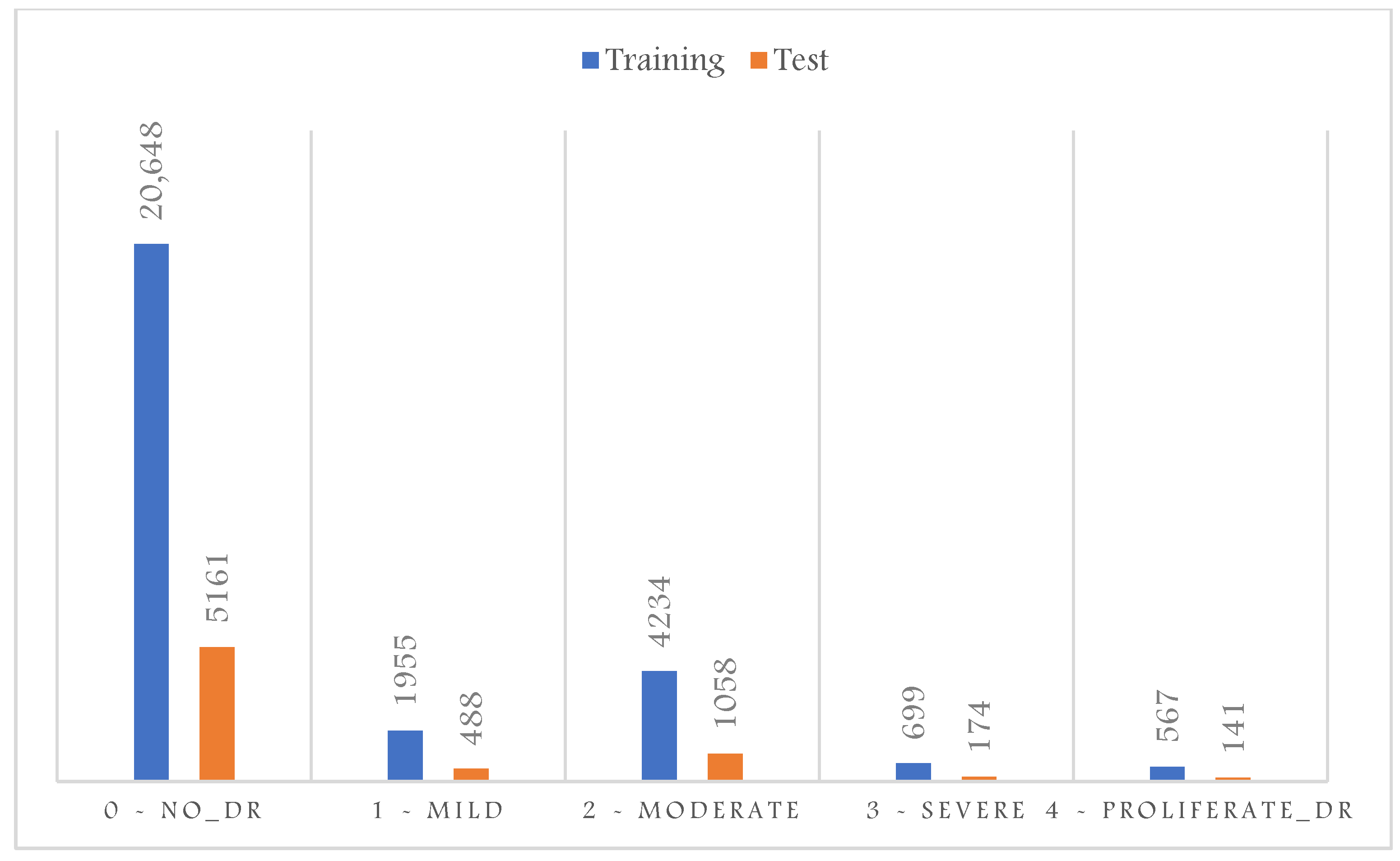
In this work, we used a publicly available dataset at Kaggle [16]. This would allow further investigation and benchmarking comparison. This dataset consists of a wide variety of retinal photographs as it was collected from multiple clinics using different cameras and over an extended period of time. The images were rated by a clinician for the severity of DR on a scale of 0 to 4: 0 for normal, 1 for mild, 2 for moderate, 3 for severe, and 4 for proliferative DR [16]. Images in this dataset may contain artifacts or are out of focus. The level of variation in this dataset introduced complexity and difficulty for any classifier model, and thus, it is very important to validate the models’ decisions. However, the dataset was originally imbalanced, and most samples belong to the normal healthy retina class. In addition, there were no samples dedicated to a validation set. Figure 2 shows the original dataset distribution consisting only of training and test sets of 28,103 and 7022 samples. Indeed, imbalanced training samples would generally lead to a naïve behavior classifier, which tends to classify the samples according to the majority class to minimize the cost function over all training samples.
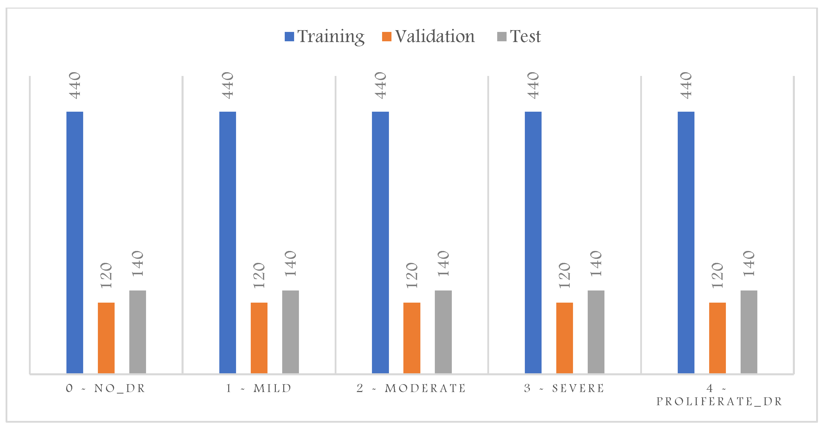
Moreover, the evaluation of imbalanced test samples is biased and misleading. Thus, to overcome this challenge, we sample three sets of training, validation, and testing to contain the same number of samples per class shown in Figure 3. The proliferative DR class contains the least number of samples; thus, the sampling for the training, validation, and test sets was based on the number of samples available for this class. This results in a total number of images in the training set of 2200, 600 for the validation, and 700 for the test set. We also converted the task into a binary classification to detect all abnormal cases in one category; thus, as shown in Figure 4, all abnormal categories were grouped.

2.2. CNN Models

The CNN models employed in this study were pre-trained on the large-scale ImageNet dataset [17], which includes 1000 categories of different objects. These models normally perform highly on general classification tasks, especially for the objects presented in the training dataset. However, their performance can be lowered when applied to specific domains, such as DR detection. In the following subsections, we start by describing the basic architecture of the CNN model. Then, we briefly describe the three pre-trained models used in this work and highlight their main characteristics.

2.2.1. Convolutional Neural Networks

CNNs are the most common artificial neural networks used for performing computing vision tasks such as image classification, object detection, and segmentation. The advantage of CNNs over other machine learning algorithms such as Support Vector Machine, K-Nearest Neighbors, Random Forest, among others, is that the CNNs can automatically learn representative features from the images and has a higher generalization capacity [18]. A CNN is typically divided into three main components: the convolutional, pooling, and dense layers. A convolutional layer learns the features and passes the features to a pooling layer to perform downsampling. A dense layer learns how to classify the extracted features into different categories. The output layer usually uses the softmax activation function to generate the probability distribution of each category in the problem domain.

2.2.2. Visual Geometry Group

The authors in [18] proposed the architecture of the Visual Geometry Group (VGG) network in 2013 and submitted their model for the 2014 ImageNet Challenge. VGG model uses a small receptive field of size 3 × 3 throughout the entire network with a 1-pixel stride. It is worth noting that the two consecutive 3 × 3 convolutional filter layers, without spatial pooling in between, provide a receptive field of size 5 × 5, and the three 3 × 3 convolutional layers filters result in a receptive field of 7 × 7. This unique characteristic allows the network to converge faster, makes the decision functions more discriminative, and reduces the number of weight parameters.

2.2.3. The Residual Network

ResNet architecture is one of the most popular and successful deep learning models for computer vision tasks. The residual network has multiple variants, including ResNet-16, ResNet-18, ResNet-34, ResNet-50, ResNet-101, ResNet-110, ResNet-152, ResNe-t164, ResNet-1202, and so forth. The residual unit is the main building block of the ResNet. The intuition behind the residual unit is to ease the costly training of the very deep networks by using a direct connection that skips some layers in between [19]. This connection is called a ‘skip connection’ or ‘shortcut connection’ and is the core of residual blocks. With the introduction of skip connection, the output is changed to F(x) + x instead of F(x) in the other layers. The skip connections in ResNet solve the vanishing gradient in deep neural networks by allowing the gradient to flow through this alternate shortcut pathway [19]. The deep ResNet is a stack of residual units seen as small neural networks with a skip connection. ResNet18 is a 72-layer architecture with 18 deep layers. The input size to the network is 224 × 224 × 3, which is predefined.

2.2.4. DenseNet-121

DenseNet is another type of CNN that uses dense connections between layers through the Dense Blocks [20]. Dense Blocks connect all layers directly with each other. However, each layer obtains additional inputs from all previous layers and passes its feature maps to all subsequent layers in a feed-forward process. DenseNets alleviate the vanishing gradient problem, encourage feature reuse, and reduce the number of learnable parameters [20]. DenseNet-121 is the simple DenseNet network designed for the ImageNet dataset. It consists of multiple dense and transition blocks. Transition Block performs as a 1 × 1 convolution with 128 filters, followed by a 2 × 2 pooling with a stride of 2, resulting in dividing the size of the volume by dividing volume size and the number of feature maps in half.

2.3. Models’ Explainability Using Grad-CAM

Deep architectures take in more than a million parameters of complex, convoluted operations. Thus, the interpretability of such algorithms is challenging. Class Activation Mapping (CAM) is one technique proposed to enhance the explainability of deep learning models. The basic idea behind CAM is to localize the deep discriminative features and visualize the object parts detected by the CNN [21].
The study in [22] inspired this idea and demonstrates that convolutional layers of CNNs behave as object detectors despite no supervision of the object’s location. To generate the CAMs, the predicted class weights are projected back to the activation maps of the previous convolutional layer to highlight class-specific discriminative regions. This approach provides visual explanations as each activation map contains different spatial information about the input, and when the convolutional layer is close to the classification layer, its activations are sufficiently high-level to provide a visual localization to explain the final decision. Let f be a CNN-based classification model and c a target category. Given an input image x and a convolutional layer of f , the CAM with respect to c can be defined as a linear combination of the activation maps of the convolutional layer, as follows [23]:
CAM c ( x ) = k = 1 N f w k c A k
where N f denotes the number of filters of the convolutional layer, A k is the kth filter of the activation, and w k c are weight coefficients indicating the importance of the activation maps with respect to the target class c . However, CAM is restricted to having a global average pooling (GAP) layer after the final convolutional layer and then a dense linear layer. The GAP computes the average of each feature map for each corresponding class, and the resulting vector is fed into the softmax activation layer, which outputs the class probabilities. If the CNN-based model does not have a GAP in the final layer, CAM requires removing the fully connected layer before the final output and replacing it with the GAP [21]. Gradient-weighted Class Activation Mapping Grad-CAM has been suggested as a generalization version of CAM, as it can be applied to any CNN-based models without modifying their architectures [23]. Similar to the CAM, Grad-CAM employs the spatial information preserved through convolutional layers to highlight the parts of an input image that are important for the classifier decisions. However, Grad-CAM uses class-specific gradient information produced by the feature maps of the last convolutional layer to generate a class-discriminative localization heatmap corresponding to a particular class [23]. The importance of feature map k   for the target class c is computed using the gradient of the logits of class c with respect to the activation maps of the final convolutional layer, and the gradients are averaged across each feature map, a ReLU nonlinearity is applied to only consider the pixels that have a positive influence on the score of the target class [23]:
L G r a d C A M c = R e L U ( k = 1 N f w k c A k )

2.4. Performance Evaluation Metrics

In this work, five evaluation metrics were employed to provide complete coverage and unbiased analysis of the results. This includes the following:
  • Accuracy: calculated as the percentage of the correctly classified images by:
    Accuracy = T P + T N   N
    where N is the total number of images in the evaluated set, T P is the true positive, i.e., detected abnormal cases, and T N is the true negative, i.e., normal cases not detected as abnormal.
  • Precision: calculated as the number of T P divided by the sum of T P and false positives, normal cases detected as abnormal.
          Precision   = T P   T P + F P
  • Sensitivity/Recall: calculated as the number of, divided by the sum of T P and false negatives F N , abnormal cases detected as normal:
          Recall   = T P   T P + F N    
  • F1-Score: defined as the harmonic mean of precision and recall:
    F 1 Score   = 2   Precision Recall     Precision + Recall  
  • Confusion matrix: A confusion matrix is a table used for summarizing a classifier’s performance. The number of correctly and incorrectly classified samples are summarized with count values and broken down by each category.

2.5. Proposed Explainability Evaluation Metric

In this paper, we propose a novel explanatory metric to validate a deep learning model’s decision, a model’s conformity that measures the proportion of model attention to DR-related lesions. To calculate a model’s conformity over the whole test set, we average the conformity of each instance in that set. We visualize the evaluated deep learning models’ Grad-CAM and evaluate the results using the conformity measure as follows:
conformity = { 1 N   i = 1 N 1 F D L i 1 + F D L i                                               w h e n   N l = 0   1 N i = 1 N T D L i T D L i + F U L i + F D L i                                 w h e n   N l > 0    
where N is the total number of images in the evaluated set, N l . is the number of DR lesion regions present in image i , T D L i   is the number of correctly detected lesions, F U L i . is the number of undetected lesions, and F D L i is the number of incorrectly detected lesions. When N l = 0   , i.e., in the case of normal images, we assume that the whole image should contribute to the classifier prediction. Thus, no specific region should be highly activated and highlighted using Grad-CAM. Therefore, the conformity   of a model, when tested on image i , equals one in this case. In contrast, if the model highlights many irrelevant regions, the conformity approaches zero. When N l > 0   , i.e., in case of abnormal images, all lesions’ regions should be highlighted using Grad-CAM. The conformity would equal one if all lesions’ regions were highlighted and approach zero if the classifier either detects false regions or misses relevant DR signs regions.

3. Results

In this study, we first compared the performance of the three models on the test set for both five classes and binary classification to see how well each model differentiates abnormal and abnormal fundus photos in these two tasks. Then, we evaluated each model’s explainability as measured by our proposed conformity metric to validate the models’ performance. We visualized the Grad-CAM outputs to compute the conformity of normal and abnormal retinal photographs. Finally, we discussed the correlation between explainability and the models’ performance.

3.1. Model Performance on the Test Set

3.1.1. Binary Classification

Table 2 presents the three models’ performance evaluation on the test and train sets for the binary classification of retinal images, i.e., whether normal or contains DR-related signs. As shown, VGG-16 resulted in the highest accuracy on the test set with the least variance between train and test set accuracies. On the other hand, Dense-Net121 clearly overfits, resulting in much lower test accuracy than training accuracy.
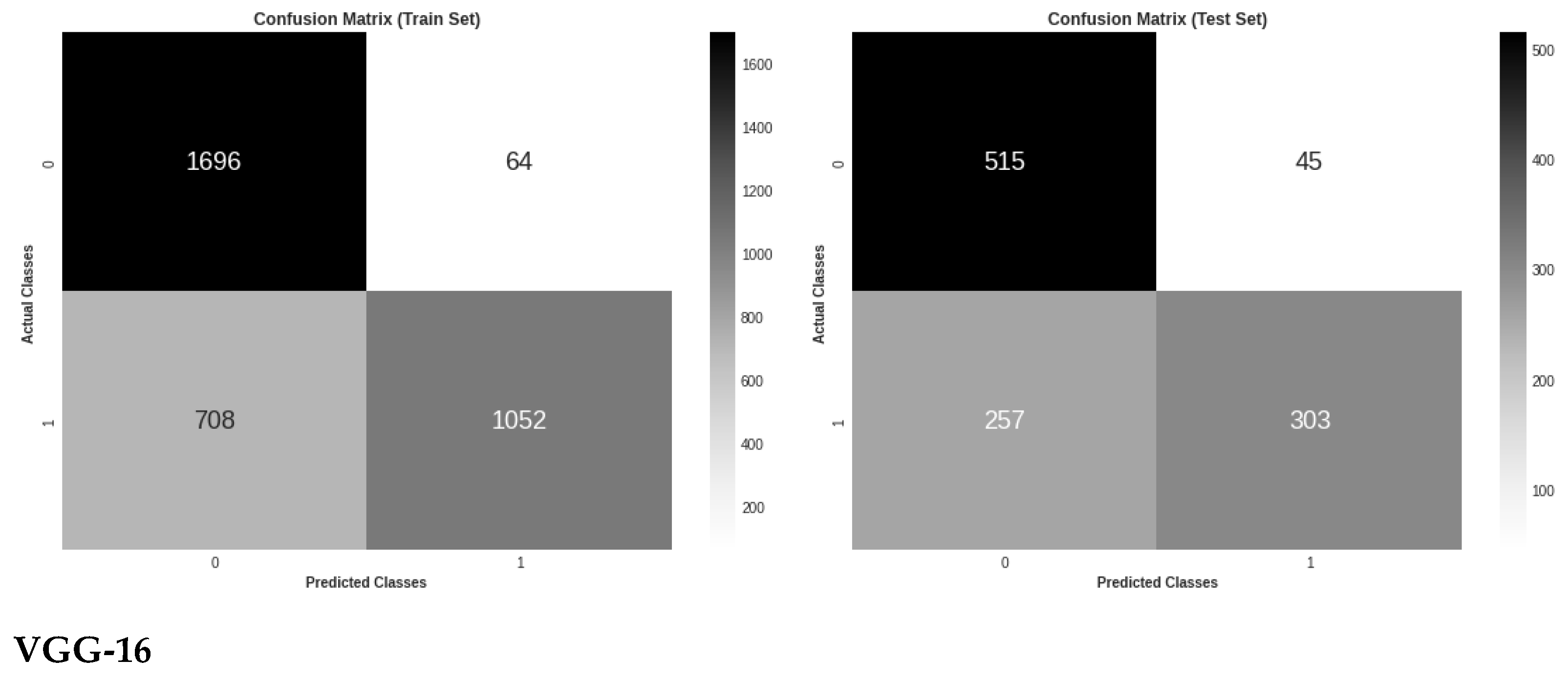
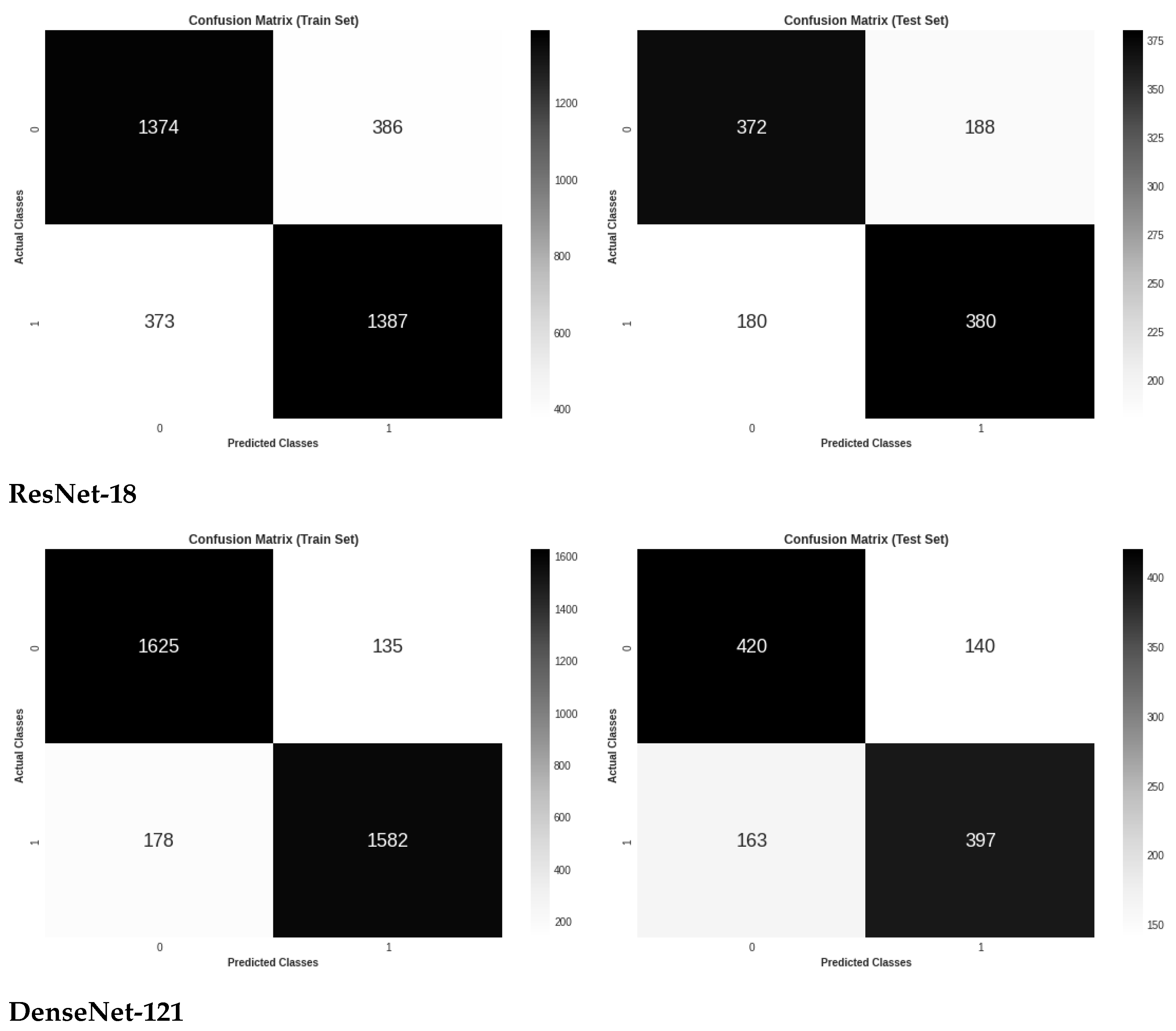
Figure 5 shows the three models’ confusion matrices on the test and train sets also for the binary classification of retinal images. As can be seen, VGG-16 resulted in the lowest number of false positives and the highest number of true positives, while ResNet-18 has the highest number of false positives and the lowest number of true positives.

3.1.2. Multiple Classification

Table 3 presents the three models’ performance evaluation on the test and train sets for the five DR stages classification of retinal images. Again, as shown, VGG-16 resulted in the highest accuracy on the test set with the least variance between train and test set accuracies, and Dense-Net121 overfitted the train set, resulting in much lower test accuracy than training accuracy.
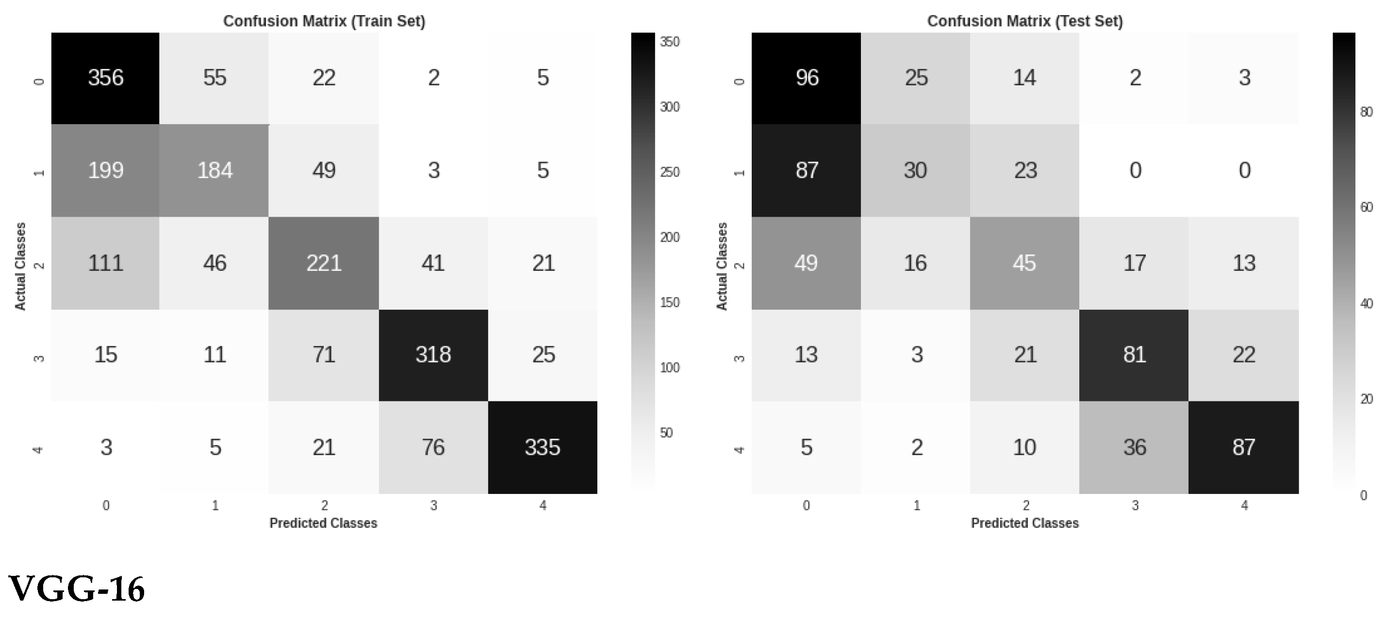
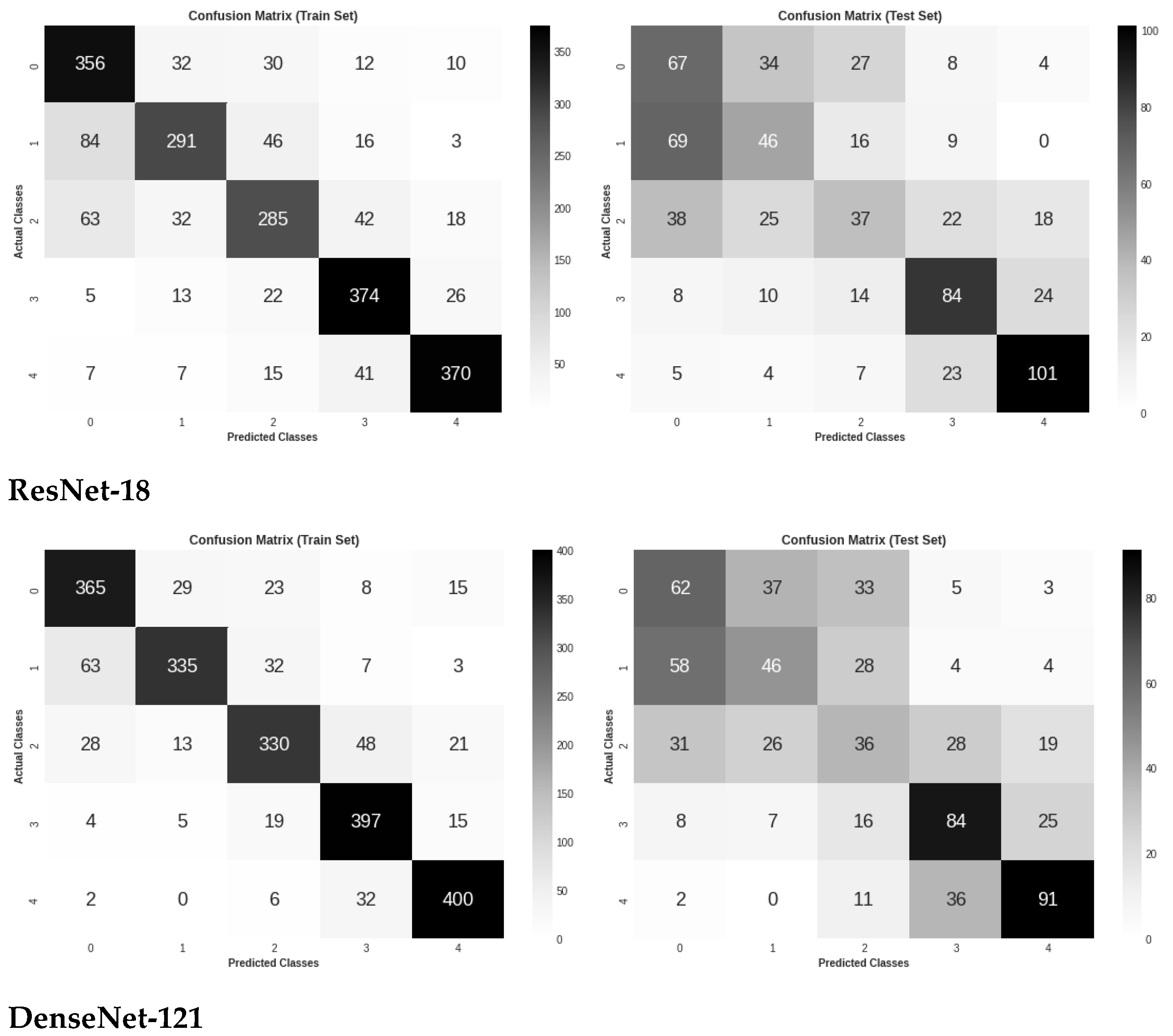
Figure 6 shows the three models’ confusion matrices on the test and train sets for the five DR stages classification of retinal images. It is worth noting that VGG-16 demonstrated the highest classification accuracy between the two early stages of DR, which might mean the ability to capture some DR lesions not seen by other models.

3.2. Models Explainability on the Test Set

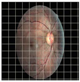
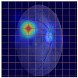
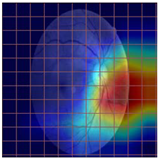
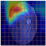
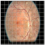
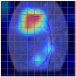
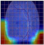
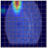
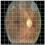
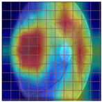
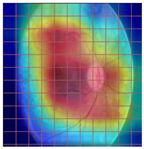
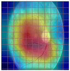
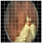
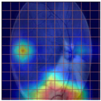
Table 4 demonstrates some examples of Grad-CAM outputs along with the original fundus photos. Table 5 presents the results of the proposed explainability metric, conformity. As can be seen from Table 4, classifiers might activate irrelevant background regions or normal retinal structures such as the optic disc or the macula. Additionally, the deep learning classifiers do not capture some clear lesion sign regions. For example, as shown in Table 4, image b, ResNet-18 model decisions were based on the background regions. Furthermore, in image c, ResNet-18 and DenseNet-121 models emphasized some irrelevant regions and failed to find DR-related signs even though the DR lesions are distinctive. Lastly, ResNet-18 and DenseNet-121 models are confused by the normal retina structure, which caused false classification by these models.

4. Discussion

In recent technological advancements, the diffusion of deep learning architectures allows for more promising results corresponding to various applications, including medical imaging and DR diagnosis. Despite achieving remarkable results in terms of model accuracies, deep learning-based methods have not achieved a significant deployment in clinical settings. One major reason is the lack of tools to inspect the decisions of deep learning models, as these models might make the right decision due to wrong reasoning. This is a serious issue, which makes it essential to give more attention to analyzing the black box nature of deep learning models. Another issue related to the performance evaluation of deep learning models in the medical field is the skewness of the data used for training and testing. This is usually due to the domination of normal over abnormal cases. Highly skewed data means the data are not evenly distributed. Machine learning models are designed to improve accuracy by reducing error and tend to produce biased and inaccurate results when faced with imbalanced datasets. Evaluation of an imbalanced dataset using accuracy metric, for example, can also be misleading as the minority class is normally the class of interest, i.e., the disease cases.
In this work, we started by creating a balanced DR dataset by obtaining the same number of instances for all classes. The main objective of dataset balancing is to train unbiased models and to have an accurate and valid evaluation. In this work, balancing data experiments reveal that the deep learning models tend to overfit the training set and do not necessarily perform well on unseen fundus photographs. This highlights the importance of giving more attention to this difficulty before feeding the algorithms with skewed data and validating the experimental results.
To overcome the challenge of unexplained predictions, we proposed a new metric that measures the models’ attention to the DR symptoms. We conducted two experiments to classify the fundus images into two and five classes. We fine-tuned three state-of-the-art deep learning architectures in both cases and visualized their decisions using Grad-CAM techniques. Our conformity metric is designed to demonstrate the models’ capability to generate a valid rationale for the classification decision. The conformity values range between 1 if all DR signs regions are highlighted by the attention techniques and approach zero if the classifier either detects false regions or misses relevant DR relevant regions. Analyzing the three fine-tuned models results in their conformity and discloses some interesting characteristics of these models and the attention methods. First, Grad-CAM, as a class-discriminative localization technique, can generate visual explanations for all three CNN-based models without requiring architectural changes or re-training. However, visualizations lend insight into the failures of these models to capture the region of interest related to the DR diagnosis task. Second, as shown in Table 2, Table 3 and Table 5, the VGG-16 model manifests the lowest generalization error and the highest conformity and explainability capabilities. This could be due to the small receptive field size used throughout the entire network and the lack of skip connections.
Third, as seen in Table 2, Table 3 and Table 5, DenseNet-121 led to the highest generalization error and overfitting of the training. Interestingly, the conformity metric of this model is the lowest compared to the other models. This emphasizes the necessity for both the data balancing step and the regularization of these models. Additionally, it highlights the correlation between the models’ performance and our proposed explainability metric.

5. Conclusions

In this paper, we evaluated three state-of-the-art models for DR binary and five-stage classification using a fundus images dataset. First, we created balanced training, validation, and test sets to ensure the validity of the evaluation results. Evaluating imbalanced sets can be misleading, especially with a skewed dataset and the domination of one class over another. Second, we optimized and fine-tuned the three models and evaluated their performance. The results show that the complexity and depth of these models make them prone to overfitting. Thus, their performance on the test degrades significantly. However, VGG-16 resulted in the least gap between training and test set accuracies and achieved the best generalization among the other models. Third, we proposed a new metric to compare the classification performance of the three models from the explainability aspect, conformity. The proposed metric utilizes the Grad-CAM technique to measure the proportion of model attention to DR-related signs. The superiority of VGG-16 was further demonstrated when evaluating the models using conformity metrics. VGG-16 achieved significantly higher conformity and showed much more justified decisions than the other models. In the future, we aim to evaluate other deep learning models’ explainability using our proposed metric and to incorporate lesion detectors with a general classifier to achieve more interpretable classification decisions.

Funding

This project was funded by the Deanship of Scientific Research (DSR) at King Abdulaziz University, Jeddah, Saudi Arabia, under Grant No. J:4-612-1441.

Institutional Review Board Statement

Not applicable.

Informed Consent Statement

Not applicable.

Data Availability Statement

Publicly available datasets were used in this study. These data can be found at https://www.kaggle.com/ratthachat/aptos-eye-preprocessing-in-diabetic-retinopathy (accessed on 4 July 2022).

Acknowledgments

The author acknowledges with thanks the DSR for technical and financial support. The author also thanks Kaggle for making the DR dataset used in this work available.

Conflicts of Interest

The author declares no conflict of interest.

References

  1. Arcadu, F.; Benmansour, F.; Maunz, A.; Willis, J.; Haskova, Z.; Prunotto, M. Deep learning algorithm predicts diabetic retinopathy progression in individual patients. NPJ Digit. Med. 2019, 2, 92. [Google Scholar] [CrossRef]
  2. WHO. Diabetes. 2021. Available online: https://www.who.int/news-room/fact-sheets/detail/diabetes (accessed on 16 July 2021).
  3. Retinopathy, D.; Understanding, D. Diabetic Retinopathy—Epidemiology Forecast to 2029. 2021, pp. 1–5. Available online: https://www.reportlinker.com/p05961707/Diabetic-Retinopathy-Epidemiology-Forecast-to.html?utm_source=GNW (accessed on 26 August 2022).
  4. Abràmoff, M.D.; Reinhardt, J.M.; Russell, S.R.; Folk, J.C.; Mahajan, V.B.; Niemeijer, M.; Quellec, G. Automated Early Detection of Diabetic Retinopathy. Ophthalmology 2010, 117, 1147–1154. [Google Scholar] [CrossRef]
  5. Chowdhury, A.R.; Chatterjee, T.; Banerjee, S. A Random Forest Classifier-Based Approach in the Detection of Abnormalities in the Retina. Med. Biol. Eng. Comput. 2019, 57, 193–203. [Google Scholar] [CrossRef] [PubMed]
  6. Bourouis, S.; Zaguia, A.; Bouguila, N.; Alroobaea, R. Deriving Probabilistic SVM Kernels from Flexible Statistical Mixture Models and its Application to Retinal Images Classification. IEEE Access 2019, 7, 1107–1117. [Google Scholar] [CrossRef]
  7. Emon, M.U.; Zannat, R.; Khatun, T.; Rahman, M.; Keya, M.S. Performance Analysis of Diabetic Retinopathy Prediction using Machine Learning Models. In Proceedings of the 2021 6th International Conference on Inventive Computation Technologies (ICICT), Coimbatore, India, 20–22 January 2021; pp. 1048–1052. [Google Scholar] [CrossRef]
  8. Zhou, J.; Gandomi, A.H.; Chen, F.; Holzinger, A. Evaluating the quality of machine learning explanations: A survey on methods and metrics. Electronics 2021, 10, 593. [Google Scholar] [CrossRef]
  9. Anoop, B.K. Binary Classification of DR-Diabetic Retinopathy using CNN with Fundus Colour Images. Mater. Today Proc. 2022, 58, 212–216. [Google Scholar] [CrossRef]
  10. Pires, R.; Avila, S.; Wainer, J.; Valle, E.; Abramoff, M.D.; Rocha, A. A data-driven approach to referable diabetic retinopathy detection. Artif. Intell. Med. 2019, 96, 93–106. [Google Scholar] [CrossRef] [PubMed]
  11. Dataset, K. Diabetic Retinopathy Detection. 2015. Available online: https://www.kaggle.com/c/diabetic-retinopathy-detection (accessed on 30 May 2022).
  12. Decencière, E.; Zhang, X.; Cazuguel, G.; Lay, B.; Cochener, B.; Trone, C.; Gain, P.; Ordonez, R.; Massin, P.; Erginay, A.; et al. Feedback on a publicly distributed database: The Messidor database. Image Anal. Stereol. 2014, 33, 231–234. [Google Scholar] [CrossRef]
  13. Wan, S.; Liang, Y.; Zhang, Y. Deep convolutional neural networks for diabetic retinopathy detection by image classification. Comput. Electr. Eng. 2018, 72, 274–282. [Google Scholar] [CrossRef]
  14. Sarki, R.; Michalska, S.; Ahmed, K.; Wang, H.; Zhang, Y. Convolutional neural networks for mild diabetic retinopathy detection: An experimental study. bioRxiv 2019, 763136. [Google Scholar] [CrossRef]
  15. Hagos, M.T.; Kant, S. Transfer Learning based Detection of Diabetic Retinopathy from Small Dataset. 2019. Available online: http://arxiv.org/abs/1905.07203 (accessed on 26 August 2022).
  16. Chatpatanasiri, R. APTOS: Eye Preprocessing in Diabetic Retinopathy. 2019. Available online: https://www.kaggle.com/ratthachat/aptos-eye-preprocessing-in-diabetic-retinopathy (accessed on 26 August 2022).
  17. Russakovsky, O.; Deng, J.; Su, H.; Krause, J.; Satheesh, S.; Ma, S.; Huang, Z.; Karpathy, A.; Khosla, A.; Bernstein, M.; et al. “ImageNet Large Scale Visual Recognition Challenge. Int. J. Comput. Vis. 2015, 115, 211–252. [Google Scholar] [CrossRef]
  18. Simonyan, K.; Zisserman, A. Very deep convolutional networks for large-scale image recognition. In Proceedings of the 3rd International Conference on Learning Representations, Conference Track Proceedings, San Diego, CA, USA, 7–9 May 2015; pp. 1–14. [Google Scholar]
  19. He, K.; Zhang, X.; Ren, S.; Sun, J. Deep residual learning for image recognition. In Proceedings of the IEEE Conference on Computer Vision and Pattern Recognition, Las Vegas, NV, USA, 27–30 June 2016; pp. 770–778. [Google Scholar] [CrossRef]
  20. Huang, G.; Liu, Z.; van der Maaten, L.; Weinberger, K.Q. Densely connected convolutional networks. In Proceedings of the 30th IEEE Conference on Computer Vision and Pattern Recognition, Honolulu, HI, USA, 21–26 July 2017; pp. 2261–2269. [Google Scholar] [CrossRef]
  21. Zhou, B.; Khosla, A.; Lapedriza, A.; Oliva, A.; Torralba, A. Learning Deep Features for Discriminative Localization. In Proceedings of the IEEE Conference on Computer Vision and Pattern Recognition, Las Vegas, NV, USA, 27–30 June 2016; pp. 2921–2929. [Google Scholar] [CrossRef]
  22. Zhou, B.; Khosla, A.; Lapedriza, A.; Oliva, A.; Torralba, A. Object detectors emerge in deep scene CNNs. In Proceedings of the 3rd International Conference on Learning Representations, Conference Track Proceedings, San Diego, CA, USA, 7–9 May 2015. [Google Scholar]
  23. Selvaraju, R.R.; Cogswell, M.; Das, A.; Vedantam, R.; Parikh, D.; Batra, D. Grad-CAM: Visual Explanations from Deep Networks via Gradient-Based Localization. Int. J. Comput. Vis. 2020, 128, 336–359. [Google Scholar] [CrossRef] [Green Version]
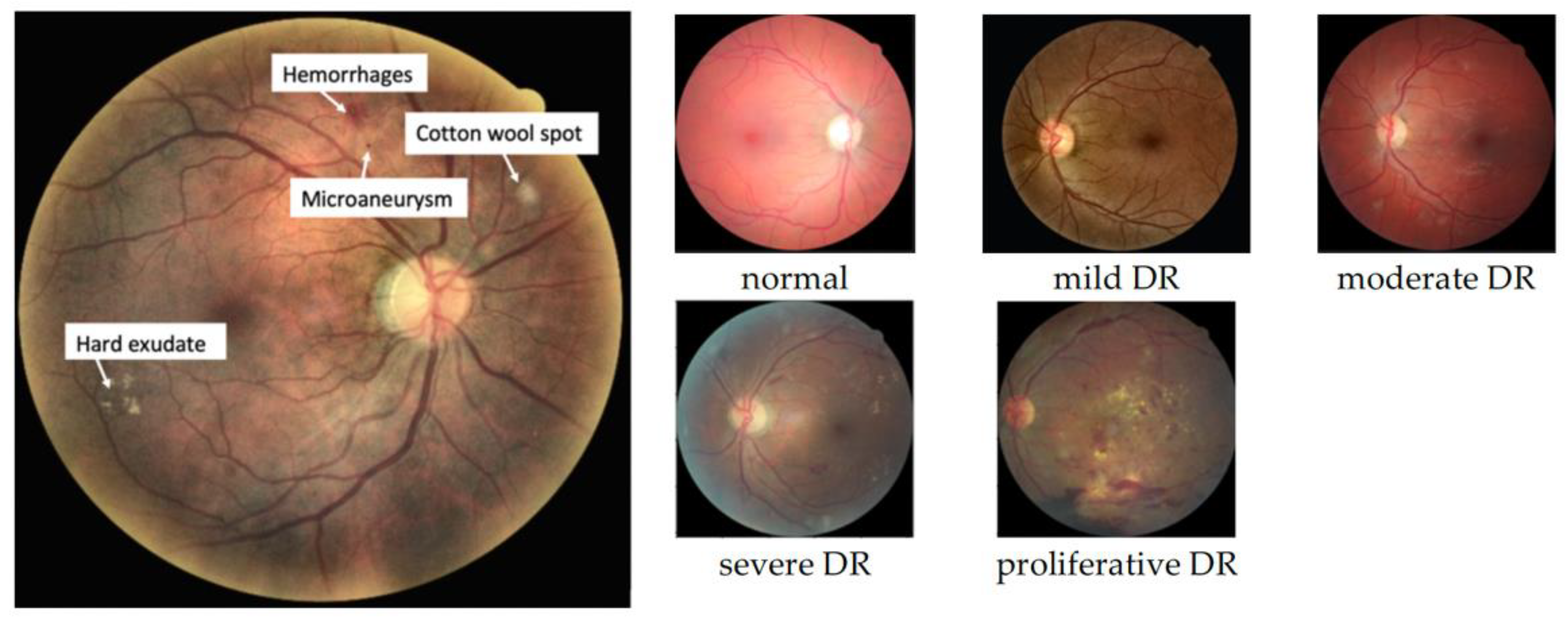
Figure 1. Different DR lesions (left) and DR stages (right).
Applsci 12 09435 g001
Figure 2. Original DR dataset distribution.
Applsci 12 09435 g002
Figure 3. DR dataset distribution after balancing the five categories.
Applsci 12 09435 g003
Figure 4. DR dataset distribution after converting it into binary categories (normal, abnormal).
Applsci 12 09435 g004
Figure 5. Confusion matrix evaluation of the three models on the test and train sets for binary classes classification.
Applsci 12 09435 g005aApplsci 12 09435 g005b
Figure 6. Confusion matrix evaluation of the three models on the test and train sets for five classes classification.
Applsci 12 09435 g006aApplsci 12 09435 g006b
Table 1. Summary of some DR automatic detection approaches applied by other related works.
Reference Dataset ApproachAccuracy
[5]DIARETDB1Random Forest93.58%
[6]Public DR datasetsSVM with Bhattacharyya kernel 91.33%
[7]MessidorLogistic Regression75.00%
[10]Kaggle DR dataset,
Messidor-2
CNN 98.20%
[13]Kaggle DR datasetAlexNet, VggNet, GoogleNet, and ResNet95.68%
[14]Kaggle DR datasetResNet50, Xception Nets, DenseNets, and VGG81.30%
[15]Kaggle DR datasetInception-V390.90%
Table 2. Performance evaluation on the test and train sets for DR detection.
Model Precision 1Recall 1F1-Score 1Train Accuracy Test Accuracy
VGG160.870.520.6578.07%73.04%
ResNet-180.670.680.6778.44%67.14%
DenseNet-1210.740.710.7391.11%72.95%
1 Calculated for the test set.
Table 3. Performance evaluation on the test and train sets for DR stages classification.
Model Precision 1Recall 1F1-Score 1Train Accuracy Test Accuracy
VGG160.450.480.4764.27% 48.43%
ResNet-180.440.480.4676.18%47.86%
DenseNet-1210.420.460.4483.05%45.57%
1 Calculated for the test set.
Table 4. Examples of Grad-CAM output of the evaluated deep learning models.
Original ImageVGG16 ResNet-18DenseNet-121
Applsci 12 09435 i001Applsci 12 09435 i002Applsci 12 09435 i003Applsci 12 09435 i004
(a)
Applsci 12 09435 i005Applsci 12 09435 i006Applsci 12 09435 i007Applsci 12 09435 i008
(b)
Applsci 12 09435 i009Applsci 12 09435 i010Applsci 12 09435 i011Applsci 12 09435 i012
(c)
Applsci 12 09435 i013Applsci 12 09435 i014Applsci 12 09435 i015Applsci 12 09435 i016
(d)
Table 5. Model conformity measures.
Model Conformity with Normal Retinal PhotosConformity with Abnormal Retinal PhotosAverage Conformity
VGG160.20000.24140.2207
ResNet-180.02940.0645 0.0469
DenseNet-1210.03850.02860.0336
Publisher’s Note: MDPI stays neutral with regard to jurisdictional claims in published maps and institutional affiliations.