Guided Random Mask: Adaptively Regularizing Deep Neural Networks for Medical Image Analysis by Potential Lesions

Abstract

Data augmentation is a critical regularization method that contributes to numerous state-of-the-art results achieved by deep neural networks (DNNs). The visual interpretation method demonstrates that the DNNs behave like object detectors, focusing on the discriminative regions in the input image. Many studies have also discovered that the DNNs correctly identify the lesions in the input, which has been confirmed in the current work. However, for medical images containing complicated lesions, we observe the DNNs focus on the most prominent abnormalities, neglecting sub-clinical characteristics that may also help diagnosis. We speculate this bias may hamper the generalization ability of DNNs, potentially causing false predicted results. Based on this consideration, a simple yet effective data augmentation method called guided random mask (GRM) is proposed to discover the lesions with different characteristics. Visual interpretation of the inference result is used as guidance to generate random-sized masks, forcing the DNNs to learn both the prominent and subtle lesions. One notable difference between GRM and conventional data augmentation methods is the association with the training phase of DNNs. The parameters in vanilla augmentation methods are independent of the training phase, which may limit their effectiveness when the scale and appearance of region-of-interests vary. Nevertheless, the effectiveness of the proposed GRM method evolves with the training of DNNs, adaptively regularizing the DNNs to alleviate the over-fitting problem. Moreover, the GRM is a parameter-free augmentation method that can be incorporated into DNNs without modifying the architecture. The GRM is empirically verified on multiple datasets with different modalities, including optical coherence tomography, x-ray, and color fundus images. Quantitative experimental results show that the proposed GRM method achieves higher classification accuracy than the commonly used augmentation methods in multiple networks. Visualization analysis also demonstrates that the GRM can better localize lesions than the vanilla network.

1. Introduction

Deep neural networks (DNNs) have revolutionized the field of medical image analysis by learning to extract high-level abstract features in a data-driven manner, rather than the conventional hand-crafted ones with limited representative ability. Both the convolutional-based [1] and Transformer-based [2] networks have achieved enormous breakthroughs in multiple medical image analysis tasks, such as disease classification, target volume segmentation, lesion detection, and image reconstruction. Based on DNNs, impressive results on numerous diseases have been reported, including the retinopathy of prematurity (ROP) [3], retinal diseases [4,5], breast cancer [6], lung diseases [7], and stomach diseases [8]. These encouraging results demonstrate that DNNs are promising methods to help design computer-aided diagnosis (CAD) systems.

Despite the progress achieved by leveraging the DNN model, the interpretability of the outputted result is a critical aspect that clinicians interested in. A CAD system that utilizes DNNs may output the classification result (e.g., benign or malignant) based on the patient’s medical imaging. However, which part of the input image associates with the output helps explain the classification result. The interpretability may also contribute to reducing the false positive or false negative samples, preventing the DNNs from failing silently when the inputs belong to the type of out-of-distribution samples [9,10]. It has been shown that the DNNs behave as object detectors, even without the supervision of the location of the object [11]. There exist several well-known visual interpretation methods that attempt to bridge the object within the input image and the output of DNNs, e.g., guided backpropagation [12], class activation mapping (CAM) [13], and gradient-weighted class activation mapping (Grad-CAM) [14]. Based on these interpretation methods, recent works show that the DNNs indeed localize the potential lesions in recognition of multiple diseases [3,15].

Figure 1 shows three OCT [4] samples that are diagnosed with CNV, accompanied by the visualization result of CAM. By observing the example in the first row, it can be found most of the lesions are located in the center of the image, and the result of CAM shows that the network accurately locates those abnormalities. Given the masked CAM shown on the right side of the first row, it is hard to determine the diagnosis since most lesions are masked. For the second and third examples, the lesions are scattered in the image, much more complicated than those in the first sample. Moreover, the corresponding CAM results indicate that the model only identified part of the lesions on the image’s right side. In the third column, green squares are used to point out the lesions ignored by the model, and the CAM-localized regions are masked. These visualization results reveal that the DNNs may bias toward the most distinguishing features in the input, ignoring other sub-clinical lesions that contain valuable information. We suspect that the above limitation may constrain the DNNs’ robustness to the variations of the lesions, causing false-negative predictions when the lesions in the image are not prominent. Ideally, it is preferred for the DNNs to recognize both the principal and subtle lesions in the input as clinicians do.

Faced with the aforementioned limitation, the core idea of the proposed method is to leverage the information contained in the CAM as a guide to discover the potential ignored lesions in the input. The visual interpretation result reveals the areas the DNNs focused on. Therefore, the rest may contains ignored sub-clinical lesions that we are interested in. To discover those lesions, a vanilla approach is to fully mask the areas indicated by the visual interpretation, enforcing the DNNs to give the prediction by utilizing the rest of the regions. This approach sounds reasonable for the second and third rows shown in Figure 1, where the DNNs are possible to predict correctly based on the lesions marked by the green squares. However, it is hard to predict the first sample based on the masked input in Figure 1, since critical information in the input is not given. A desirable approach is to moderately mask the potential lesions with the help of visual interpretations without the complete loss of valuable information. Thus, the DNNs can adapt to the inputs that contain either simplified or complicated lesions. Based on this consideration, this paper proposes a simple yet effective data augmentation method called guided random mask (GRM), which randomly masks the areas indicated by the visual interpretation during the training phase. The term “guided” in GRM refers to the information provided by the visual interpretation, and “random mask” implies the stochasticity that produces the effect of regularization.

The proposed GRM is a data augmentation method that can prevent the DNNs from focusing only on prominent input lesions and can better utilize spatial contextual information. Notably, the GRM is a parameter-free method that can accommodate lesions with different scales and complexity. It is known that data augmentation plays a vitally important role in the training of DNNs to mitigate the problem of over-fitting. One inspiration of the proposed GRM is the cutout [16], which randomly masks the input with a fixed size area and helps the DNNs achieve state-of-the-art performance on CIFAR [17] and SVHN [18] datasets. However, compared with the CIFAR and SVHN with relatively small image sizes (32 × 32), it is much harder to apply the cutout to high-resolution medical images because of the hyper-parameter tuning. The hyper-parameter in the cutout is the size of the mask, which can be regarded as the strength of regularization in training DNNs. Its optimal value is task-dependent and requires grid search to achieve the best performance, which may limit its effectiveness in practice. On the contrary, the proposed GRM eliminates the difficulty in hyper-parameter tuning by using the guidance provided by the visual interpretation. Unlike the fixed mask size in cutout, the one in the proposed GRM is adaptively adjusted along with the training of DNNs, making it applicable to recognition tasks with varied scales and complexity of lesions.

The contributions of the paper can be summarized as follows:

(i)

We found that the DNNs may bias toward the most prominent features and ignore the sub-clinical ones when the input image contains complicated lesions.

(ii)

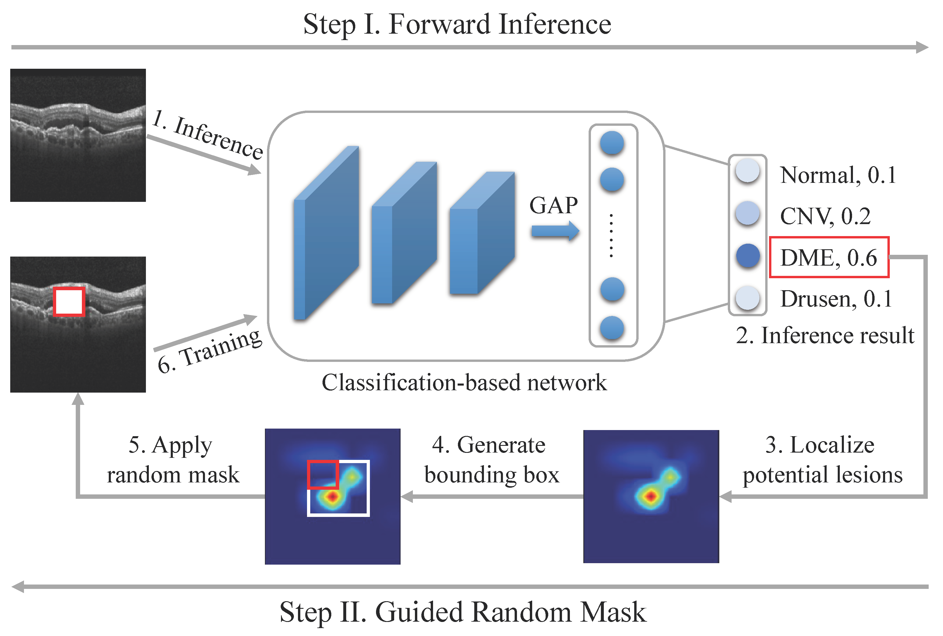
A parameter-free data augmentation method called GRM is proposed, which utilizes visual interpretation of the prediction result to regularize the training of DNNs adaptively.

(iii)

Visual interpretation demonstrates that DNNs coupled with GRM can more effectively utilize the contextual information than the vanilla models.

(iv)

Ablation studies on multiple datasets, including OCT, X-ray, and ultrasound images, empirically show that the GRM substantially surpasses the benchmark method on various tasks.

The rest of the paper is organized as follows. Section 2 summarizes the related works about the applications in medical imaging and common augmentation methods used for the training of DNNs. Section 3 first illustrates the three types of medical imaging datasets used, followed by a detailed explanation of the proposed method. Section 4 shows the results of extensive experiments, including the comparison of the baseline model and other well-known related augmentation methods. Visualization analysis is also used to verify the effectiveness of the GRM. Finally, Section 5 summarizes and concludes the GRM. The source code is available at https://github.com/hujunjiescu/GRM, accessed on 1 January 2022.

2. Related Works

2.1. DNNs in Medical Image Analysis

DNNs have become ubiquitous methods in the field of medical image analysis, where Deep Convolutional Neural Networks (DCNNs) [1,19,20] and the recently emerged Vision Transformer (ViT) [2] are the two most prevalent paradigms. The following two paragraphs briefly demonstrate their applications in medical image analysis tasks.

For the DCNNs, starting from 2012 when AlexNet [19] won the ILSVRC-2012 competition [21], many breakthroughs in vision-related tasks have been achieved using DCNNs. Several key factors contribute to the success of DCNNs, including massive annotated high-quality datasets, powerful computation capability by utilizing graphics processing units (GPUs), and novel architectures. Multiple architectures of DCNNs proposed in the natural image field have also been successfully applied in medical images. For example, Inception-V3 [22] has been used to identify the retinal diseases in OCT images [4]. Experimental results demonstrate that DCNNs outperform some human experts and can aid in expediting the diagnosis in clinical practice. A three-stage DCNNs-based architecture is proposed in [3] to recognize the existence of ROP based on the fundus images, where multiple popular architectures including VGG [23], GoogLeNet [20], and ResNet [1] delivered promising performance. A novel network architecture called U-Net is proposed in [24] to accomplish biomedical segmentation tasks in an end-to-end manner, surpassing the compared methods by a large margin. This tremendous success makes the U-Net a benchmark in biomedical segmentation tasks. Lots of U-Net’s variations have lately been proposed by incorporating attention mechanism [15,25,26], residual convolution blocks [27], etc. Besides the applications in disease diagnoses, DCNNs have also achieved remarkable progress in image reconstruction [28], denoising [29,30], etc.

Transformer [31] is an attention-based model that was initially proposed to solve machine translation tasks. It achieves better performance than the conventional recurrent models, raising expectations that it may also be applicable to the image field. Many researchers attempt to bridge the gap between natural language processing (NLP) and vision, and ViT [2] is one of the well-known Transformer-based models that achieves promising results on the natural image classification task. In addition to the natural image-related tasks, Transformer has also been gaining attention in medical image analysis. Hatamizadeh et al. [32] proposes a Transformer-based segmentation architecture called UNETR that combines the U-Net [24] with Transformer to accomplish the volumetric segmentation task. It achieves the state-of-the-art performance on the dataset of Multi-Atlas Labeling Beyond The Cranial Vault [33] and Medical Segmentation Decathlon (MSD) [34]. A relation Transformer network (RTNet) is proposed in [35] that leverage the Transformer to exploit and interact with the relationships between the lesions and vessels. TransMed is proposed in [36] to incorporate the advantages of DCNNs and Transformer to perform the classification task of multi-model medical image. By combining the feature extraction ability of DCNNs and the spatial relationship modeling capacity of Transformer, TransMed achieves better accuracy than conventional DCNNs-based models.

Even the Transformer delivered competitive performance compared with DCNNs: [37] recently showed that a pure DCNN can surpass the state-of-the-art Transformer by deliberately designing the DCNN’s component and architecture. It is hard to say which one is more overwhelming than another since both the DCNNs and Transformers have unique advantages in object recognition.

2.2. Augmentation Methods for Training DCNNs

A massive annotated dataset is an indispensable factor for the success of DNNs since both the DCNNs and Transformers typically have millions of parameters, implying the potential over-fitting problem when the amount of training dataset is limited. During the training phase, it is common to utilize regularization methods to alleviate the over-fitting risk, thus improving the generalization ability. Data augmentation, which aims to increase the diversity of training data, is a frequently used regularization method that contributes to many state-of-the-art results on both natural and medical image analysis tasks.

Current data augmentation methods mainly focus on the domains of spatial and intensity. In the spatial domain, the random crop and flip for the CIFAR [17] dataset have become the standard operations during the training phase [1,16]. U-Net [24] shows that excessive data augmentation by applying elastic deformation to the training dataset is critical for biomedical segmentation, particularly when the number of training samples is limited. For the intensity domain, common augmentation methods include brightness enhancement [38], color transformation [39], noise injection [40], blurring [41] etc. In addition to the domains of spatial and intensity, another type of effective augmentation method is mixup [42], which generates new training samples through the convex combination of random paired examples and their labels. Mixup and its variant [43] have also been applied to medical image segmentation tasks.

Perhaps one of the closest works to ours is the cutout approach [16], which augments the spatial domain by randomly masking squared regions in the input image. Cutout can be regarded as a variant of dropout [44] that randomly drops neurons during the training phase to reduce co-adaptations. Instead of dropping neurons in the dropout, cutout randomly drops squared pixels in the input image. Despite the progress brought by the cutout, one of its limitations lies in the difficulty of determining the optimal masked size (suppose is r) in the input image. The target size varies from the task, indicating that the optimal value of r is task-dependent and can only be determined by trial-and-error. The main reason behind this issue is the separation between the data augmentation and the training phase of DNNs. The proposed GRM method eliminates the problem by leveraging the guidance from the visual interpretation to determine the augmentation parameters, thus bridging the gap between the data augmentation and the training phase. The proposed GRM method has two significant advantages over the cutout. First, the GRM can adaptively adjust the size of the mask with the guidance of visual interpretation without specifying the hyper-parameter r. Second, the GRM can efficiently utilize the contextual information and discover the potential sub-clinical lesions by masking the target region. Essentially, the GRM can be regarded as a regularizer that alleviates the over-fitting problem.

3. Data and Methodology

3.1. Data

Three types of medical imaging datasets are used in the experiments, including OCTs of retinal diseases, X-rays of pneumonia, and color fundus images of glaucoma.

Table 1. Statistics of the used three medical imaging datasets.

	Part	Modality	Task	Classes	Training Samples	Validation Samples	Test Samples
Retinal diseases	Eyes	OCT	Classification	4	4000	1000	1000
Pneumonia	Chest	X-ray	Classification	2	4632	600	624
Glaucoma	Eyes	Color fundus image	Classification	2	5232	744	744

summarizes the subset of these three datasets used in the experiments. The retinal diseases dataset comprises four classes, i.e., normal, choroidal neovascularization (CNV), diabetic macular edema (DME), and drusen. The pneumonia dataset contains two classes: normal and pneumonia. Similar to the pneumonia dataset, the glaucoma dataset includes normal and glaucoma as the two classes. All three datasets are open source. The retinal diseases and pneumonia dataset can be downloaded at https://data.mendeley.com/datasets/rscbjbr9sj/3, accessed on 1 January 2022, and the glaucoma dataset can be downloaded at https://doi.org/10.5281/zenodo.5793241, accessed on 1 January 2022. Illustrations of these three datasets can be found in Figure 2. Each dataset is manually split into three parts, including training, validation, and test datasets. The experimental results are reported on the test dataset by using the model that achieves the best metric on the validation part.

3.2. Methodology

The proposed GRM is a data augmentation method that bridges the augmentation characteristics with the training phase of the model to identify the ignored sub-clinical lesions adaptively. Two problems need to be solved to achieve the adaptive regularization effect, that is (1) how to discover the region of interest (ROI) that indicates the location of the potential lesions and (2) how to utilize the information contained in the ROI. The corresponding solutions to the two problems are demonstrated in the following subsections.

3.2.1. Localizing Potential Lesions

Consider the C-classes classification task based on DNNs, including the DCNNs and Transformers. Given the input image $\mathit{x}$, the DNNs denoted as $F(\mathit{x};\mathit{W})$ would output the prediction result ${\mathit{a}}^L$ after the layer-by-layer forward computation, where L denotes the number of layers in the DNNs. ${\mathit{a}}^L$ is a vector in the length of C, whose elements indicate the probability of each class. Generally, the largest component in ${\mathit{a}}^L$, suppose ${\mathit{a}}_c^L$, would be the category assigned to the input $\mathit{x}$. What we are interested in is which part in the $\mathit{x}$ contributes to the class c.

There are multiple ways to solve the above problem. Here, the CAM [13] is utilized for its computational efficiency and simplicity. An essential component in the CAM is the global average pooling (GAP), which is first proposed in the NIN [45] architecture to reduce the use of fully connected (FC) layers. The GAP average the feature maps along the dimension of the channel to reduce the features from a three-dimensional tensor to a one-dimensional vector. In the modern architecture of DNNs, it is common to use the GAP in the penultimate layer to get the global representation of the input, followed by an FC layer whose dimension is C. The core idea of CAM can be regarded as the reverse computation of the above steps, where the learnable weight in the last FC layer (which can be considered as the importance of feature per channel) is used to weight the extracted features to indicate which part in the input is associated with the prediction.

Formally, suppose the features fed into the GAP are denoted as ${\mathit{a}}^{L-1}$ in the shape of $[K,W,H]$ that indicate the number of channels, width, and height, respectively. ${\mathit{W}}^{L-1}$ represents the learnable weight within the last FC layer in the shape of $[C,K]$. The probability of class c is then given by the softmax equation ${\mathit{a}}_c^L=\frac{exp\left({\mathit{z}}_c^L\right)}{{\sum }_{i=1}^{C}exp\left({\mathit{z}}_i^L\right)}$. The scalar variable ${\mathit{z}}_c^L$ is computed as:

$${\mathit{z}}_c^L=\sum _{k=1}^K{\mathit{W}}_{c,k}^{L-1}·\sum _{w=1}^W\sum _{h=1}^H{\mathit{a}}_{k,w,h}^{L-1}.$$

(1)

The summation on the right side of the above equation represents the GAP, which can be regarded as the feature’s context representation along the dimension of the channel. The parameter ${\mathit{W}}^{L-1}$ thus indirectly represents the contribution of each channel in the ${\mathit{a}}^{L-1}$ to the predicted score. By leveraging the information contained in ${\mathit{W}}^{L-1}$ to integrate ${\mathit{a}}^{L-1}$ in a channel-wise way, it is then possible to highlight the probable areas corresponding to the predicted class. This computation process can be formulated as:

$${\mathit{M}}_c=\sum _{k=1}^K{\mathit{W}}_{c,k}^{L-1}·{\mathit{a}}_k^{L-1},$$

(2)

where ${\mathit{M}}_c$ denotes the CAM for class c. Each channel in ${\mathit{a}}^{L-1}$ represents a visual pattern discovered by DNNs. Therefore the CAM can be considered as a weighted summation of the presence of each visual pattern at different spatial locations. Note that the CAM represents the visual pattern in the feature-level’s spatial resolution, which is much smaller than the input image. The CAM is required to be upsampled to the resolution of the input image in order to identify the image regions corresponding to the predicted category.

3.2.2. Guided Random Mask

Having identified the possible lesions indicated by the CAM, the next problem to be tackled is how to utilize it to regularize the training of DNNs. We aim to realize moderate regularization effectiveness, that is, to avoid entirely masking the lesions that may cause strong regularization or mask regions with a fixed size that introduce an extra hyper-parameter. Based on this consideration, we propose mask regions with a random size guided by CAM. Figure 3 illustrates the overall computation steps of the proposed GRM method. First, the inference of the input image is required in order to identify its category and locate the potential lesions, which is indicated by the procedures of 1, 2, 3. The next step is generating the bounding box of the CAM, which embodies the majority of regions with high values in CAM. The bounding box of CAM is computed from the binarized CAM, which is accomplished by using the 90th percentile of the original CAM (i.e., a pixel larger than the 90th percentile is 1, otherwise it 0). Then we randomly choose the central point in the bounding box and allocate the width and height with their maximum value the same as that in the bounding box. The bounding box of CAM and randomly generated mask are shown as the white and red boxes in Figure 3, respectively. Finally, the random mask is applied to the raw input by setting the area in the input to 0, later used to train the DNNs. Note that the GRM method is only used in the training phase, not including the test phase.

The above computation processes are designed for the classification task, where its application to segmentation tasks is straightforward. The inference computation to compute CAM can be omitted for the segmentation task since the target is precisely described in the label. It only requires finding the bounding box of the target and generating a corresponding random mask within it. The introduced computational cost is negligible and can be implemented as the preprocessing procedure.

The computational process of the proposed GRM is summarized in Algorithm 1.

Algorithm 1: Algorithm of the proposed GRM method for the classification task.

4. Experimental Setup and Results

4.1. Experimental Setup

Multiple modern network architectures including Inception-V3 [22], ResNet-50 [1], DenseNet-121 [46], and ViT [2] are used to verify the generalization of the GRM method. The cross-entropy is used as the cost function for the classification tasks. For the CNNs (ResNet-50, Inception-V3, and DenseNet-121), Adadelta [47] is used as the optimizer to minimize the cost function, where the learning rate is set to 1.0. For the ViT, AdamW [48] is used as the optimizer, coupled with a cosine decay learning rate scheduler and 20 epochs of linear warm-up. The learning rate is set to 0.0001. The size of the image is fixed as 224 for all the experiments.

The number of training epochs is set to 300, which is long enough for the convergence of training. All networks are implemented by using PyTorch [49]. The experiments are carried out on a server with Linux OS and CPU Intel Xeon E5-2620 @2.4GHz, four NVIDIA TITAN RTX GPUs, and 64 GB of RAM.

4.2. Ablation Studies of GRM

To verify the effectiveness of the proposed GRM method, we first quantitatively compare the network with and without the GRM.

Table 2. Comparison of accuracy (%) between the vanilla networks and the one applied with GRM on the three medical image analysis tasks.

Task	Network	Vanilla	GRM
Retinal diseases	Inception-V3	94.9	96.7
	ResNet-50	93.7	96.3
	DenseNet-121	93.6	96.0
	ViT	89.9	92.6
Pneumonia	Inception-V3	90.4	92.8
	ResNet-50	90.0	94.2
	DenseNet-121	88.8	92.1
	ViT	90.2	91.8
Glaucoma	Inception-V3	89.2	91.6
	ResNet-50	87.5	90.6
	DenseNet-121	88.9	90.0
	ViT	87.5	88.5

shows the accuracy of multiple networks on the three tasks. For the vanilla network, it can be found that the Inception-V3 achieves the highest accuracy among all the tasks. For example, the accuracy of Inception-V3 on retinal diseases is $94.9$, far beyond the $89.9$ of the ViT. The inferiority of ViT can be attributed to the difficulty in hyper-parameter tuning and the limited size of the medical image dataset, which significantly increase the risk of over-fitting. By comparing the vanilla network with the one with GRM applied, it can be observed that the accuracy of GRM is unanimously improved among all the tasks, regardless of the network architecture. The highest improvement is from $90.0$ to $94.2$ in the ResNet-50 on the pneumonia task. A varying degree of improvement is also obtained for the ViT in the three datasets. These encouraging results illustrate that the proposed GRM is broadly applicable to datasets composed of varied modalities and class numbers.

One of the reasons for the effectiveness of GRM is the adaptive regularization, which helps the network better extract the context information and alleviate the over-fitting issue. To delve into the training procedure, Figure 4 summarizes the training and validation loss of ResNet-50 in the three tasks. It can be observed the regularization effectiveness brought by GRM in the task of retinal diseases in Figure 4a, where the training loss of GRM (red dotted line) decreases slower than the one in the vanilla network (red solid line), implying the GRM helps to mitigate over-fitting to the training dataset. On the contrary, the validation loss of GRM (green dotted line) is distinctly lower than the one of baseline (green solid line), demonstrating that the GRM increases the network’s generalization capacity. Similar convergence results can be found in the pneumonia task. The effectiveness of GRM can also be notably found in the glaucoma task, where the validation loss of the vanilla ResNet-50 increases rapidly from the 50th epoch, and its ascending speed goes faster along the training epochs. This convergence behavior can be commonly observed in the training of networks. By adding GRM to the network, the stability of validation loss is significantly improved, as shown in the green dotted line in Figure 4c. These convergence results confirmed the regularization impact brought by the GRM, which helps combat the over-fitting issue on the training dataset and boosts the generalization ability on the validation dataset.

4.3. Comparison between GRM with Other Augmentation Methods

To further validate the effectiveness of the GRM, we also compare it with cutout [16] and mixup [42]. As shown in

Table 3. Comparison of accuracy (%) between the GRM and related methods on the three medical image analysis tasks.

Task	Network	GRM	Cutout	Mixup
Retinal diseases	Inception-V3	96.7	94.3	95.8
	ResNet-50	96.3	94.1	92.8
	DenseNet-121	96.0	95.1	95.6
	ViT	92.6	92.0	92.8
Pneumonia	Inception-V3	92.8	89.2	91.2
	ResNet-50	94.2	89.7	91.5
	DenseNet-121	92.1	92.0	91.0
	ViT	91.8	91.1	89.1
Glaucoma	Inception-V3	91.6	89.0	91.4
	ResNet-50	90.6	87.3	89.4
	DenseNet-121	90.0	89.6	88.8
	ViT	88.5	86.2	86.1

, the GRM is superior to the cutout in improving the diagnosis accuracy. The most significant improvement happens in the Inception network for retinal diseases, which raises the accuracy from $94.3$ to $96.7$. For pneumonia and glaucoma diseases, different degrees of improvement can also be found in various networks. Experimental results in Table 3 also demonstrate the advantage of GRM over mixup. It can be observed that the GRM outperforms mixup in most tasks except the ViT of retinal diseases, where the accuracy of mixup is $92.8$, marginally higher than the $92.6$ of GRM. One significant advantage of the GRM and cutout lies in the adaptivity to the inputs. The mask size in the cutout is fixed, whereas the GRM can adaptively adjust the size and location of the mask according to the input. For the Mixup, it combines paired inputs and labels convexly to alleviate the overfitting problem, which can be used together with GRM to increase the capacity of the networks.

4.4. Visualization Analysis

The motivation of GRM roots in the potential bias of the vanilla network, which attempts to capture the most prominent characteristics of lesions and may ignore the sub-clinical ones. To demonstrate whether the GRM can remit the issue or not, Figure 5 compares the visualization results between the vanilla network and the one applied with GRM on five retinal diseases cases. The first row represents a relatively simple sample that contains abnormals in the center of the image. It can be found that both of the two networks have precisely identified the lesions. For the sample shown in the second row, it can be seen that the vanilla network biases to the right-most lesions and neglects the abnormals located in the center. On the contrary, the GRM has accurately discovered most of the lesions. Similar results can be observed in the third sample. For the fourth sample containing complicated lesions, the vanilla network biases the right-bottom areas, while the GRM has precisely identified intricate lesions. In the fifth sample, both networks found the most distinguished lesion on the right side, whereas only the GRM has identified the nearby subtle lesions.

These visualization results demonstrate two points. First, the DNNs are object detectors that attempt to discover the abnormalities in the input image. It performs well in those images that contain prominent characteristics, such as the sample shown in the first row in Figure 5. Second, the vanilla DNNs may fail to capture the prominent and subtle lesions simultaneously for the image comprised of complicated features. With the help of GRM, the DNNs can efficiently utilize the context information and show much better performance than the vanilla network.

5. Conclusions

This paper proposes a simple yet effective data augmentation method named GRM that aims to discover the potential sub-clinical lesions ignored by the DNNs. The visual interpretation results are used as guidance to help locate the ROIs. Random masking of those ROIs enforces the DNNs to better utilize the context information. Moreover, it also increases the DNNs’ robustness to the input since the model is required to predict the category from the incomplete input. Conventional data augmentation method (e.g., cutout) requires to specify the size of the mask, which increases the difficulty during practice when the size of the target varies. On the contrary, the proposed GRM adaptively changes the size and location of the mask according to the characteristics of the target.

Ablation experiments on multiple network architectures are carried out to validate the effectiveness of GRM. The GRM can substantially increase the networks’ recognition accuracy on different tasks compared to the vanilla network. The network applied with GRM exhibits evident lower loss on the validation dataset, implying that the GRM helps to increase the networks’ generalization capacity. Visualization experiments further demonstrate that the GRM contributes to exploit the sub-clinical lesions and helps reduce the false predictions during practice. In the training phase, the GRM leverages the CAM of the inference result as guidance to randomly mask the input, which is later used to train the network. From a more general point of view, the GRM can be applied iteratively, i.e., the inference and training of the sample can be repeated multiple times till the stability of CAM is achieved. The iterative method may contribute to the learning process of the network because of the enhanced regularization effectiveness. The exploration of the iterative version of GRM is left as a future work.

References

1. He, K.; Zhang, X.; Ren, S.; Sun, J. Deep residual learning for image recognition. In Proceedings of the IEEE Conference on Computer Vision and Pattern Recognition, Las Vegas, NV, USA, 27–30 June 2016; pp. 770–778. [Google Scholar]
2. Dosovitskiy, A.; Beyer, L.; Kolesnikov, A.; Weissenborn, D.; Zhai, X.; Unterthiner, T.; Dehghani, M.; Minderer, M.; Heigold, G.; Gelly, S.; et al. An Image is Worth 16 × 16 Words: Transformers for Image Recognition at Scale. In Proceedings of the International Conference on Learning Representations, Virtual, 26 April–1 May 2020. [Google Scholar]
3. Hu, J.; Chen, Y.; Zhong, J.; Ju, R.; Yi, Z. Automated analysis for retinopathy of prematurity by deep neural networks. IEEE Trans. Med. Imaging 2018, 38, 269–279. [Google Scholar] [CrossRef] [PubMed]
4. Kermany, D.S.; Goldbaum, M.; Cai, W.; Valentim, C.C.; Liang, H.; Baxter, S.L.; McKeown, A.; Yang, G.; Wu, X.; Yan, F.; et al. Identifying medical diagnoses and treatable diseases by image-based deep learning. Cell 2018, 172, 1122–1131. [Google Scholar] [CrossRef] [PubMed]
5. Hu, J.; Chen, Y.; Yi, Z. Automated segmentation of macular edema in OCT using deep neural networks. Med. Image Anal. 2019, 55, 216–227. [Google Scholar] [CrossRef] [PubMed]
6. Wang, Z.; Zhang, L.; Shu, X.; Lv, Q.; Yi, Z. An end-to-end mammogram diagnosis: A new multi-instance and multiscale method based on single-image feature. IEEE Trans. Cogn. Dev. Syst. 2020, 13, 535–545. [Google Scholar] [CrossRef]
7. Anthimopoulos, M.; Christodoulidis, S.; Ebner, L.; Christe, A.; Mougiakakou, S. Lung pattern classification for interstitial lung diseases using a deep convolutional neural network. IEEE Trans. Med. Imaging 2016, 35, 1207–1216. [Google Scholar] [CrossRef]
8. Lu, Y.; Chen, Y.; Zhao, D.; Liu, B.; Lai, Z.; Chen, J. CNN-G: Convolutional neural network combined with graph for image segmentation with theoretical analysis. IEEE Trans. Cogn. Dev. Syst. 2020, 13, 631–644. [Google Scholar] [CrossRef]
9. DeVries, T.; Taylor, G.W. Learning confidence for out-of-distribution detection in neural networks. arXiv 2018, arXiv:1802.04865. [Google Scholar]
10. Jiang, H.; Kim, B.; Guan, M.; Gupta, M. To trust or not to trust a classifier. In Advances in Neural Information Processing Systems; The MIT Press: Cambridge, MA, USA, 2018; pp. 5541–5552. [Google Scholar]
11. Zhou, B.; Khosla, A.; Lapedriza, A.; Oliva, A.; Torralba, A. Object detectors emerge in deep scene cnns. arXiv 2014, arXiv:1412.6856. [Google Scholar]
12. Springenberg, J.T.; Dosovitskiy, A.; Brox, T.; Riedmiller, M. Striving for simplicity: The all convolutional net. arXiv 2014, arXiv:1412.6806. [Google Scholar]
13. Zhou, B.; Khosla, A.; Lapedriza, A.; Oliva, A.; Torralba, A. Learning deep features for discriminative localization. In Proceedings of the IEEE Conference on Computer Vision and Pattern Recognition, Las Vegas, NV, USA, 27–30 June 2016; pp. 2921–2929. [Google Scholar]
14. Selvaraju, R.R.; Cogswell, M.; Das, A.; Vedantam, R.; Parikh, D.; Batra, D. Grad-cam: Visual explanations from deep networks via gradient-based localization. In Proceedings of the IEEE International Conference on Computer Vision, Venice, Italy, 27–29 October 2017; pp. 618–626. [Google Scholar]
15. Yang, H.; Kim, J.Y.; Kim, H.; Adhikari, S.P. Guided soft attention network for classification of breast cancer histopathology images. IEEE Trans. Med. Imaging 2019, 39, 1306–1315. [Google Scholar] [CrossRef]
16. DeVries, T.; Taylor, G.W. Improved regularization of convolutional neural networks with cutout. arXiv 2017, arXiv:1708.04552. [Google Scholar]
17. Krizhevsky, A.; Hinton, G. Learning Multiple Layers of Features from Tiny Images; Citeseer: State College, PA, USA, 2009. [Google Scholar]
18. Netzer, Y.; Wang, T.; Coates, A.; Bissacco, A.; Wu, B.; Ng, A.Y. Reading digits in natural images with unsupervised feature learning. In Proceedings of the NIPS Workshop on Deep Learning and Unsupervised Feature Learning, Granada, Spain, 16 December 2011. [Google Scholar]
19. Krizhevsky, A.; Sutskever, I.; Hinton, G.E. Imagenet classification with deep convolutional neural networks. In Advances in Neural Information Processing Systems; The MIT Press: Cambridge, MA, USA, 2012; pp. 1097–1105. [Google Scholar]
20. Szegedy, C.; Liu, W.; Jia, Y.; Sermanet, P.; Reed, S.; Anguelov, D.; Erhan, D.; Vanhoucke, V.; Rabinovich, A. Going deeper with convolutions. In Proceedings of the IEEE Conference on Computer Vision and Pattern Recognition, Boston, MA, USA, 7–12 June 2015; pp. 1–9. [Google Scholar]
21. Deng, J.; Dong, W.; Socher, R.; Li, L.J.; Li, K.; Li, F.F. ImageNet: A large-scale hierarchical image database. In Proceedings of the IEEE Conference on Computer Vision and Pattern Recognition, Miami, FL, USA, 20–25 June 2009; pp. 248–255. [Google Scholar]
22. Szegedy, C.; Vanhoucke, V.; Ioffe, S.; Shlens, J.; Wojna, Z. Rethinking the inception architecture for computer vision. In Proceedings of the IEEE Conference on Computer Vision and Pattern Recognition, Las Vegas, NV, USA, 27–30 June 2016; pp. 2818–2826. [Google Scholar]
23. Simonyan, K.; Zisserman, A. Very deep convolutional networks for large-scale image recognition. arXiv 2014, arXiv:1409.1556. [Google Scholar]
24. Ronneberger, O.; Fischer, P.; Brox, T. U-net: Convolutional networks for biomedical image segmentation. In Proceedings of the International Conference on Medical Image Computing and Computer-Assisted Intervention, Munich, Germany, 5–9 October 2015; Springer: Berlin/Heidelberg, Germany, 2015; pp. 234–241. [Google Scholar]
25. Oktay, O.; Schlemper, J.; Folgoc, L.L.; Lee, M.; Heinrich, M.; Misawa, K.; Mori, K.; McDonagh, S.; Hammerla, N.Y.; Kainz, B.; et al. Attention u-net: Learning where to look for the pancreas. arXiv 2018, arXiv:1804.03999. [Google Scholar]
26. Roy, A.G.; Navab, N.; Wachinger, C. Concurrent spatial and channel ‘squeeze & excitation’ in fully convolutional networks. In Proceedings of the International Conference on Medical Image Computing and Computer-Assisted Intervention, Granada, Spain, 16–20 September 2018; Springer: Berlin/Heidelberg, Germany, 2018; pp. 421–429. [Google Scholar]
27. Alom, M.Z.; Hasan, M.; Yakopcic, C.; Taha, T.M.; Asari, V.K. Recurrent residual convolutional neural network based on u-net (r2u-net) for medical image segmentation. arXiv 2018, arXiv:1802.06955. [Google Scholar]
28. Shan, H.; Padole, A.; Homayounieh, F.; Kruger, U.; Khera, R.D.; Nitiwarangkul, C.; Kalra, M.K.; Wang, G. Competitive performance of a modularized deep neural network compared to commercial algorithms for low-dose CT image reconstruction. Nat. Mach. Intell. 2019, 1, 269–276. [Google Scholar] [CrossRef]
29. Yang, Q.; Yan, P.; Zhang, Y.; Yu, H.; Shi, Y.; Mou, X.; Kalra, M.K.; Zhang, Y.; Sun, L.; Wang, G. Low-dose CT image denoising using a generative adversarial network with Wasserstein distance and perceptual loss. IEEE Trans. Med. Imaging 2018, 37, 1348–1357. [Google Scholar] [CrossRef]
30. Shan, H.; Zhang, Y.; Yang, Q.; Kruger, U.; Kalra, M.K.; Sun, L.; Cong, W.; Wang, G. 3-D convolutional encoder-decoder network for low-dose CT via transfer learning from a 2-D trained network. IEEE Trans. Med. Imaging 2018, 37, 1522–1534. [Google Scholar] [CrossRef]
31. Vaswani, A.; Shazeer, N.; Parmar, N.; Uszkoreit, J.; Jones, L.; Gomez, A.N.; Kaiser, Ł.; Polosukhin, I. Attention is all you need. In Advances in Neural Information Processing Systems; The MIT Press: Cambridge, MA, USA, 2017; Volume 30. [Google Scholar]
32. Hatamizadeh, A.; Tang, Y.; Nath, V.; Yang, D.; Myronenko, A.; Landman, B.; Roth, H.R.; Xu, D. UNETR: Transformers for 3D Medical Image Segmentation. In Proceedings of the IEEE/CVF Winter Conference on Applications of Computer Vision, Waikoloa, HI, USA, 4–8 January 2022; pp. 574–584. [Google Scholar]
33. Landman, B.; Xu, Z.; Igelsias, J.; Styner, M.; Langerak, T.; Klein, A. MICCAI multi-atlas labeling beyond the cranial vault–workshop and challenge. In Proceedings of the MICCAI Multi-Atlas Labeling Beyond Cranial Vaul—Workshop Challenge, Munich, Germany, 5–9 October 2015; Volume 5, p. 12. [Google Scholar]
34. Simpson, A.L.; Antonelli, M.; Bakas, S.; Bilello, M.; Farahani, K.; Van Ginneken, B.; Kopp-Schneider, A.; Landman, B.A.; Litjens, G.; Menze, B.; et al. A large annotated medical image dataset for the development and evaluation of segmentation algorithms. arXiv 2019, arXiv:1902.09063. [Google Scholar]
35. Huang, S.; Li, J.; Xiao, Y.; Shen, N.; Xu, T. RTNet: Relation Transformer Network for Diabetic Retinopathy Multi-lesion Segmentation. IEEE Trans. Med. Imaging 2022, 41, 1596–1607. [Google Scholar] [CrossRef]
36. Dai, Y.; Gao, Y.; Liu, F. Transmed: Transformers advance multi-modal medical image classification. Diagnostics 2021, 11, 1384. [Google Scholar] [CrossRef]
37. Liu, Z.; Mao, H.; Wu, C.Y.; Feichtenhofer, C.; Darrell, T.; Xie, S. A ConvNet for the 2020s. arXiv 2022, arXiv:2201.03545. [Google Scholar]
38. Dong, H.; Yang, G.; Liu, F.; Mo, Y.; Guo, Y. Automatic brain tumor detection and segmentation using u-net based fully convolutional networks. In Proceedings of the Annual Conference on Medical Image Understanding and Analysis, Edinburgh, UK, 11–13 July 2017; Springer: Berlin/Heidelberg, Germany, 2017; pp. 506–517. [Google Scholar]
39. Liskowski, P.; Krawiec, K. Segmenting retinal blood vessels with deep neural networks. IEEE Trans. Med. Imaging 2016, 35, 2369–2380. [Google Scholar] [CrossRef] [PubMed]
40. Christ, P.F.; Elshaer, M.E.A.; Ettlinger, F.; Tatavarty, S.; Bickel, M.; Bilic, P.; Rempfler, M.; Armbruster, M.; Hofmann, F.; D’Anastasi, M.; et al. Automatic liver and lesion segmentation in CT using cascaded fully convolutional neural networks and 3D conditional random fields. In Proceedings of the International Conference on Medical Image Computing and Computer-Assisted Intervention, Athens, Greece, 17–21 October 2016; Springer: Berlin/Heidelberg, Germany, 2016; pp. 415–423. [Google Scholar]
41. Sirinukunwattana, K.; Pluim, J.P.; Chen, H.; Qi, X.; Heng, P.A.; Guo, Y.B.; Wang, L.Y.; Matuszewski, B.J.; Bruni, E.; Sanchez, U.; et al. Gland segmentation in colon histology images: The glas challenge contest. Med. Image Anal. 2017, 35, 489–502. [Google Scholar] [CrossRef]
42. Zhang, H.; Cisse, M.; Dauphin, Y.N.; Lopez-Paz, D. mixup: Beyond empirical risk minimization. arXiv 2017, arXiv:1710.09412. [Google Scholar]
43. Bdair, T.; Navab, N.; Albarqouni, S. ROAM: Random Layer Mixup for Semi-Supervised Learning in Medical Imaging. arXiv 2020, arXiv:2003.09439. [Google Scholar] [CrossRef]
44. Srivastava, N.; Hinton, G.; Krizhevsky, A.; Sutskever, I.; Salakhutdinov, R. Dropout: A simple way to prevent neural networks from overfitting. J. Mach. Learn. Res. 2014, 15, 1929–1958. [Google Scholar]
45. Lin, M.; Chen, Q.; Yan, S. Network in network. In Proceedings of the International Conference on Learning Representations, Scottsdale, AZ, USA, 2–4 May 2013. [Google Scholar]
46. Huang, G.; Liu, Z.; Van Der Maaten, L.; Weinberger, K.Q. Densely connected convolutional networks. In Proceedings of the IEEE Conference on Computer Vision and Pattern Recognition, Honolulu, HI, USA, 21–26 July 2017; pp. 4700–4708. [Google Scholar]
47. Kingma, D.; Ba, J. ADADELTA: An Adaptive Learning Rate Method. arXiv 2012, arXiv:1212.5701. [Google Scholar]
48. Loshchilov, I.; Hutter, F. Decoupled Weight Decay Regularization. In Proceedings of the International Conference on Learning Representations, Vancouver, BC, Canada, 30 April–3 May 2018. [Google Scholar]
49. Paszke, A.; Gross, S.; Chintala, S.; Chanan, G.; Yang, E.; DeVito, Z.; Lin, Z.; Desmaison, A.; Antiga, L.; Lerer, A. Automatic differentiation in PyTorch. In Proceedings of the 31st Conference of Advances in Neural Information Processing Systems, Long Beach, CA, USA, 4–9 December 2017; Available online: ttps://openreview.net/forum?id=BJJsrmfCZ (accessed on 30 July 2022).
Figure 1. Three choroidal neovascularization (CNV) samples containing a neovascular membrane. Each row represents an optical coherence tomography (OCT) sample. The three columns denote the original OCT image, the visualization result of CAM, and the image with CAM masked, respectively. For the right-most image in all three rows, the white masks represent the result area of CAM, and the green squares denote the lesions ignored by DNNs. Detailed illustration of dataset and computation principle of CAM can be found in Section 3.
Applsci 12 09099 g001
Figure 2. Characteristics of different classes in the three datasets.
Applsci 12 09099 g002
Figure 3. Computation procedures of the proposed GRM method for the classification task.
Applsci 12 09099 g003
Figure 4. Convergence comparison between the vanilla ResNet-50 and ResNet-50 applied with the proposed GRM on the retinal disease, pneumonia, and glaucoma tasks, respectively.
Applsci 12 09099 g004
Figure 5. Qualitative comparison between the vanilla ResNet-50 and the ResNet-50 applied with the proposed GRM on five retinal disease cases. Each row denotes a case.
Applsci 12 09099 g005