Article

Crack Extension Analysis of Atmospheric Stress Corrosion Based on Peridynamics

1
School of Mechanical Engineering, Guizhou University, Guiyang 550025, China
2
State Key Laboratory of Public Big Data, Guizhou University, Guiyang 550025, China
*
Author to whom correspondence should be addressed.
Appl. Sci. 2022, 12(19), 10008; https://doi.org/10.3390/app121910008
Submission received: 7 September 2022 / Revised: 29 September 2022 / Accepted: 29 September 2022 / Published: 5 October 2022

Abstract

:
Based on peridynamics, an atmospheric stress corrosion model was proposed. In this model, the role of hydrogen and stress in anodic-dissolution-dominated stress corrosion cracking was considered, and atmospheric corrosion was characterized by the change in liquid film thickness on the metal surface in the atmospheric environment. The near-field kinetic anodic dissolution model and the atmospheric corrosion model were coupled by varying the liquid film thickness. The thickness of the liquid film depended on factors such as the temperature, relative humidity, and hygroscopic salts. We validated the model using stress corrosion behavior from the literature for 304 stainless steel in a simulated atmospheric environment. The results of the model captured the crack expansion process. The obtained crack expansion direction and branching behavior agreed well with the experimental results in the literature.

1. Introduction

Atmospheric stress corrosion (ASCC) is the phenomenon of the stress corrosion cracking (SCC) of metals in the atmospheric environment and is one of the most prevalent and hazardous forms of metal corrosion. Metallic materials are subject to varying degrees of atmospheric corrosion from raw material inventory and component processing to assembly and service. Some common examples can be observed in land, water, and air transportation systems; electronic circuit boards; and urban and marine infrastructure. The degradation of metals due to atmospheric exposure has a significant impact on society [1]. According to recent reports, economic losses due to corrosion are estimated to be 3.4% of the global GDP, and losses due to atmospheric corrosion failure account for approximately more than 50% of losses in the overall corrosion field [2].
Stress corrosion cracking (SCC) is the process of rupture of a metallic material under the combined effect of stress and the corresponding environment. Stress corrosion cracking occurs in many common metallic materials in the corresponding environment, and in some harsh stress corrosion systems, stress corrosion in the material can even occur within a few minutes. The initial formation of SCC is microcracking, followed by the continuous expansion and fusion of microcracks to form macroscopic cracks. The environments in which SCC occurs are usually acidic, alkaline, and high-temperature water.
According to the corrosion mechanism, SCC is split into two types: anodic dissolution (AD) and hydrogen embrittlement (HE) [3]. Regarding the AD mechanism, under the combined influence of stress and the medium, the metal is dissolved by electrochemical reactions in the medium, resulting in crack creation and extension. The AD stress corrosion mechanism includes the slip dissolution mechanism, oxide film cracking mechanism, selective dissolution mechanism, and corrosion-promoted plastic deformation mechanism [4,5]. In the hydrogen embrittlement mechanism, hydrogen atoms diffuse into the metal matrix and become trapped by various hydrogen traps [6]. The metal matrix exposed to hydrogen becomes brittle due to reduced ductility, followed by cracking under stress. The hydrogen-enhanced debonding process, hydrogen-enhanced local plasticity, adsorption-induced dislocation emission, hydride production, cleavage, and other HE stress corrosion mechanisms are the most common [7,8,9,10].
During the atmospheric stress corrosion of metals, the variation of thin-film electrolyte thickness is a major factor in determining the corrosion rate and corrosion mechanism [11,12,13,14,15,16]. For example, the corrosion rates of iron [14,16] and steel [17,18,19,20] are significantly higher in uniform electrolyte thicknesses of 10–30μm than in monolithic electrolyte or immersion conditions [14,16,17,18,19,20], and the maximum corrosion rate of zinc occurs at electrolyte thicknesses of 8–10μm [21,22]. However, the thickness of thin-film electrolytes is affected by many factors, such as the temperature, relative humidity, wind, rainfall, and contaminants in the air and on the metal surface [23,24,25,26,27]. These environmental factors have an important influence on the thickness of the electrolyte, and this influence is both profound and extremely complex. The complexity is mainly due to the following reasons: these environmental factors are not constant and change dynamically, not only with time but also with spatial shifts; the effects of these environmental factors on the electrolyte thickness are not independent of each other but interact with each other. Furthermore, these environmental factors interact with each other and cause dynamic changes in each other.
ASCC has become an important research area for stainless steel because of the characteristics of sudden onset, large damage, and being difficult to monitor. Simulating the crack sprouting and expansion in materials plays an important role in the reliability analysis and health monitoring of engineering structures. Most of the existing numerical models for simulating crack emergence and expansion in materials are based on the finite element method (FEM). In the conventional finite element method, the displacement field discontinuity generated by the crack expansion is corrected by redefining the object. That is, the crack is defined as a boundary and the mesh needs to be re-defined after each crack extension. It is also necessary to provide mathematical expressions for the kinetic relationships that control crack growth for the simulated fracture method to describe how the crack expands under local conditions. Considering the above factors, it is difficult to solve the multi-crack problem with multiple interactions and a complex expansion mode using the traditional finite element method.
The extended finite element method (XFEM) [28] is one of the ways to solve these challenges by introducing additional nodal degrees of freedom and local strengthening functions on top of the standard finite elements. These reinforcement functions contain discontinuous displacement fields and can simulate the growth of cracks and fractures without the need to divide the mesh. However, this approach requires the reintroduction of external criteria. Meanwhile, the XFEM model performs poorly in terms of crack sprouting and fracture. Molecular dynamics simulation (MDS) [29] uses interatomic forces to simulate crack sprouting and extension, and is a detailed and realistic method for predicting material fracture. However, because of computational capacity constraints, the time and size scales that can be studied in simulations differ greatly from those required in real-world engineering applications.
Peridynamics (PD) was proposed by Silling et al. [30], who constructed new elastodynamic equations based on space integral equations and the idea of nonlocal action. The theory has unique advantages when dealing with damage and fracture problems by solving spatial integral equations to simulate mechanical behavior. It also has a strong ability to capture complex phenomena. Examples include crack nucleation, crack spreading, multi-crack joining, and crack halting in both isotropic and non-isotropic materials [31]. In PD theory, cracks can naturally sprout and expand freely without imposing a restriction criterion on crack expansion [32]. PD theory has been widely used in the simulation of crack initiation and extension in a variety of materials. PD corrosion models were shown to be a reliable and flexible tool for simulating corrosion damage and were used for damage evolution in pitting and intergranular corrosion in a variety of alloys [33,34,35,36].
Siavash Jafarzadeh et al. [36] coupled a PD corrosion model with a PD mechanics model to simulate the mechanochemical effects of stress on the anodic dissolution rate. Dennj De Meo et al. [31] proposed a numerical multi-physics field near-field kinetic framework for simulating the stress corrosion cracking of adsorbed hydrogen based on the AIDEC mechanism. Ziguang Chen et al. [37] proposed a PD model of stress corrosion that was dominated by an anodic dissolution mechanism. Xiu Ran et al. [38] simulated the hydrogen embrittlement of AISI 4340 steel. However, their simulation and experimental models were conducted by submerging the samples in an electrolyte solution and did not consider the stress corrosion cracking of metallic materials in an atmospheric environment, i.e., ASCC. Meanwhile, in their PD models, hydrogen embrittlement or anodic dissolution was singled out as the only mechanism for the occurrence of the stress corrosion of metals. However, according to relevant studies, anodic dissolution and hydrogen embrittlement do not exist in isolation when SCC occurs. The effects of anodic dissolution and hydrogen atoms are simultaneous and interact during stress corrosion [39,40,41,42,43,44], and the dominant mechanism of stress corrosion may also change when the environmental medium is changed [45,46,47]. Katona, R M et al. [48] experimentally confirmed the importance of hydrogen precipitation reactions during atmospheric corrosion.
There were two innovations in this study: (1) the application of PD in ASCC and (2) the introduction of a new PD model that organically combines the synergistic effects of anodic dissolution and hydrogen atoms in stress corrosion for the simulation of the ASCC of 304 stainless steel.

2. Materials and Methods

A peridynamics atmospheric stress corrosion model was proposed for the first time. In this model, the role of hydrogen and stress in anodic-dissolution-dominated stress corrosion cracking was considered, and atmospheric corrosion was characterized by the change in liquid film thickness on the metal surface in the atmospheric environment. The near-field kinetic anodic dissolution model and the atmospheric corrosion model were coupled by varying the liquid film thickness. We validated the model using stress corrosion behavior in the literature for 304 stainless steel in a simulated atmospheric environment.

2.1. Atmospheric Stress Corrosion Coupling Model with Peridynamics

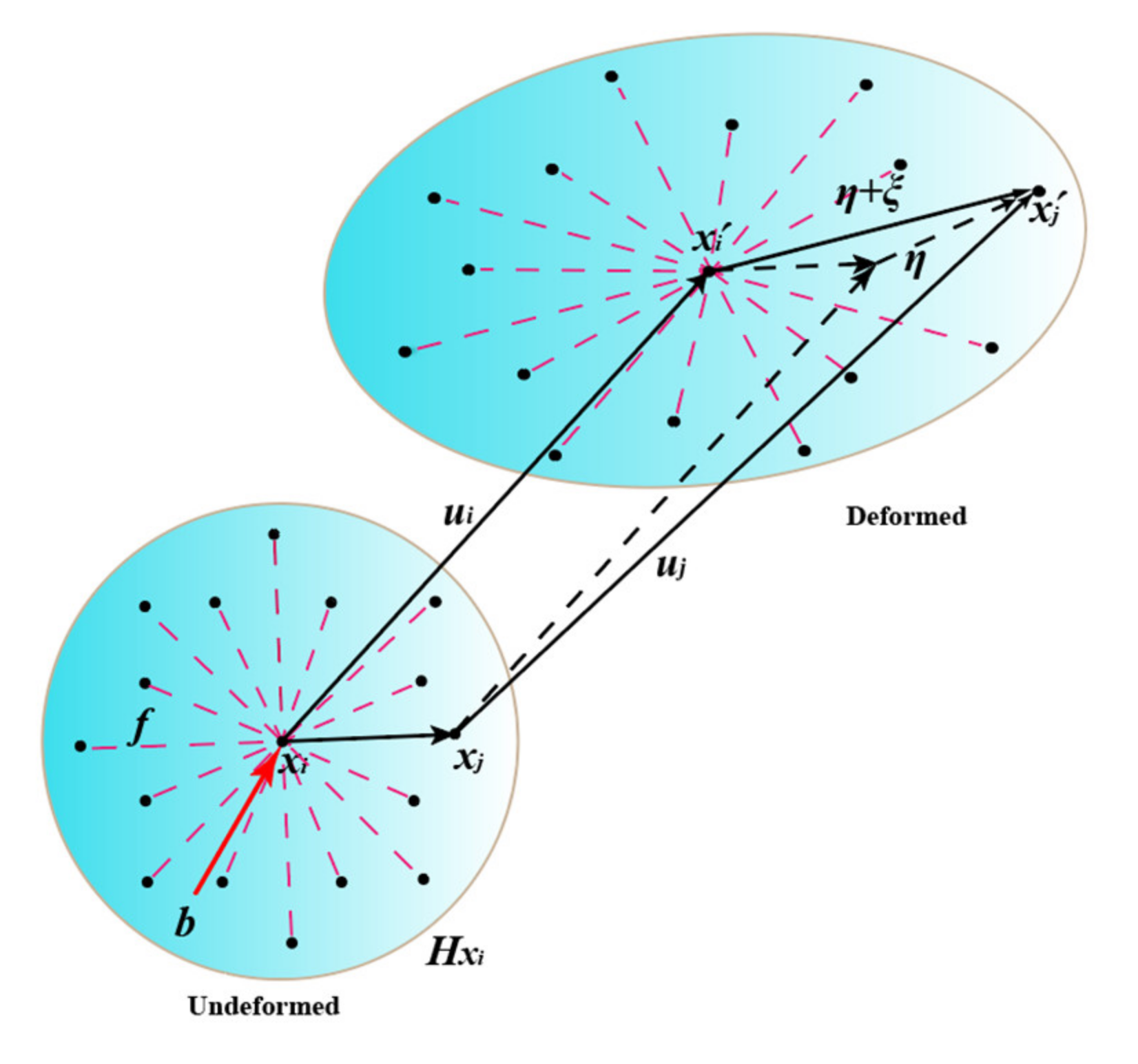
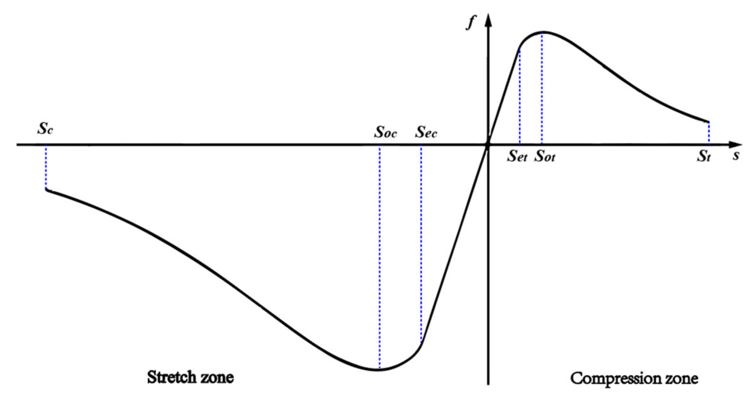
2.1.1. Peridynamics Fracture Model

In the peridynamics theory proposed by Silling et al. [30], it is assumed that the material is composed of material points that are uniformly distributed in space. At any time, each material point in the material represents the position of a material particle, and each particle has its particle volume and mass density. Particles move and deform when they are affected by a force and velocity. Peridynamics involves the study of the motion of objects due to the interaction between particles in objects. It is assumed that the interaction force between a particle x i and a particle beyond a certain range (near field range δ) is negligible, and the particles within its near field range are called family H x i . PD theory studies the interaction between a particle and all particles within its near-field range.
The existence of interaction between the mass point x i and all the mass points in the family H x i produces a force density vector that acts on the mass point x i , which can be regarded as a force that is applied to the mass point x i by the mass point x j . Similarly, the mass point x j is acted upon by all the other mass points in the family H x j . In the bonded peridynamics theory, a bond describes the interaction between two material locations, and a broken bond means that there is no longer an interaction force between the mass points. The mass points act in pairs, and the relative position state changes of two interacting material points when they are subjected to external forces are shown in Figure 1: x i and x j denote the initial positions of two material points, and x i and x j denote the positions of two mass points after a certain time t of external forces.
The fundamental equations of motion for near-field dynamics are constructed based on Newton’s second law. The mechanical parameters and characteristics of the materials are incorporated into the fundamental equations of motion through the instanton equations to achieve numerical simulations of damage to different materials. u i denotes the displacement of matter point x i , where its unit is m , while u j denotes the displacement of matter point x j , m . Let η and ξ represent the relative displacement and relative position of the material point x i and material point x j , respectively, where the expressions are ξ = x j x i and η = u x j , t u x i , t = x j x j x i x i , m . Within the theoretical framework of bonded peridynamics, the equation of motion of the material point x i in time t can be formulated as [49]
ρ i x i u ¨   i x i , t = H x i   f η , ξ , t d V j + b i x i , t , x j H
where ρ i denotes the mass density of matter point x i , k g / m 3 ; b i denotes the external load in terms of the body force density (force per unit volume of matter), N / m 3 ; H x i is the near-field range of matter point x i ; V j is the volume of matter point x j , m 3 ; ρ i x i u ¨   i x i , t represents the combined force that affects matter point x i ; and H x i f η , ξ , t d V j represents the sum of the bond forces acting with all matter points in the near-field region H x i of matter point x i .
The force density vector f η , ξ , t represents the inter-mass point-to-point force response function, i.e., the intrinsic force function, which is defined as the force vector per unit volume squared applied to the mass point x i by the mass point x j , N / m 6 . For austenitic steels, which undergo quasi-dissociative brittle fracture in a hydrogen environment, the initial microscopic elastic–brittle (PMB) model can be used, in which the relationship between the force density vector f and the elongation S is a combination of being linear and nonlinear, as shown in Figure 2.
Combining the results of Silling et al. [50] and Jianfeng Wang et al. [51], the present constitutive equation can be expressed as
f   η , ξ = C 1 S   e x p S S e c S o c C 2 η + ξ η + ξ ,                 S c   S < S e c C 1 S C 2 η + ξ η + ξ ,                                                                       S e c   S S e t   C 1 S   e x p S S e t S o t C 2 η + ξ η + ξ ,                 S e t < S S t   0 ,                                                                                                                             o t h e r s
where S e t denotes the linear elastic elongation of the bond in tension and S e c denotes the linear elastic elongation of the bond in compression, corresponding to the elastic deformation part of the material; S o t and S o c are the critical elongation of the bond in tension and compression, respectively, corresponding to the maximum value of the near-field force; S t and S c are the fracture elongation of the bond in tension and compression, respectively, corresponding to the fracture of the bond; S is the elongation of the bond, which can be interpreted as strain in classical continuum medium theory; C 1 and C 2 are peridynamic material parameters, N / m 6 ; S , C 1 , and C 2 are calculated as shown below:
S = η + ξ ξ ξ
C 1 = C = 6 E π δ 4 1 2 v
C 2 = C α
where E is Young’s modulus, v is Poisson’s ratio, the bond constant C 1 is equivalent to the “modulus of elasticity” of the material in elastodynamics, and α is the coefficient of thermal expansion of the material. The failure criterion of PD includes the critical bond elongation criterion and the critical bond energy criterion. The critical elongation S 0 is the extreme value of the bond deformation and can be solved based on the assumption that the fracture is completely separated and there is no other form of energy dissipation near the crack tip. It is calculated as
S 0 = 10 G 0 π c δ 5
G 0 is the critical energy release rate, N / m   , and is calculated as follows:
G 0 = K I C 2 E / 1 ν 2
Bond fracture occurs when S S 0   . Any material point is impacted by some bonds within its near-field range. If the bonds acting on the material point in the region of the near field break, the damage increases. The damage of a material point x at moment t can be expressed as
φ = n d n
where n d denotes the number of bonds that were broken in the near-field region of the material point and n denotes the total number of bonds in the near-field region of the material point.
In many practical applications, cracks are present at the beginning or distributed in several parts of the structure; therefore, we use the PD method to prefabricate these initial cracks. This is also a common method used in studies related to near-field dynamics.

2.1.2. Atmospheric Corrosion Model

The atmospheric corrosion of metals is a phenomenon that is prevalent in nature; it is very different from the corrosion of metals in their native solution, with the main difference being the thickness of the electrolyte liquid film on the surface of the metal. According to the thickness of the liquid film, atmospheric corrosion is divided into three categories:
(1)
Dry atmospheric corrosion: There is no liquid film coating on the metal surface. It is mostly generated by pure chemical reactions and its corrosion efficiency and destruction are often modest.
(2)
Humid atmospheric corrosion: There is a 10 nm–1 μ m liquid film coating on the metal surface. This thin liquid film is generated on a metal surface via capillary action, adsorption, or chemical condensation. Atmospheric oxygen travels considerably more readily through the water film on the metal surface than through the liquid layer when totally submerged.
(3)
Wet atmospheric corrosion: There is a 1 μ m –1 mm liquid film coating on the metal surface. It is broadly compatible with the electrochemical corrosion mechanism in the body solution.
The main research objects of atmospheric corrosion are humid and wet atmospheric corrosion. They fundamentally belong to the same category as corrosion in the native solution: electrochemical corrosion. During the atmospheric corrosion of metals, the variation of the film electrolyte thickness ( λ ) is the main determinant of the corrosion rate. The atmospheric corrosion rate increases with the liquid film thickness and then decreases. When the liquid film thickness is λ 0 , the corrosion rate reaches a maximum and then gradually becomes smaller. This is mainly due to the liquid film being too thick, preventing the oxygen in the air from diffusing through the electrolyte solution to the metal surface where the anodic reaction occurs. At this time, the oxygen reduction reaction at the cathode begins to be blocked and the reduction reaction of hydrogen begins to occur.
The anodic reaction of atmospheric corrosion is
M M n + + n e
When the electrolyte layer is very thin, the cathodic process is dominated by the oxygen reduction reaction, and the hydrogen precipitation reaction can be disregarded. The cathodic process is
O 2 + 2 H 2 O + 4 e 4 O H
For a higher electrolyte thickness of λ 0 , the oxygen reduction reaction is blocked and hydrogen precipitation begins to occur in the cathodic process:
2 H + + 2 e H 2
Van den Steen, N et al. [14] proposed a dynamic electrolyte film corrosion model based on the continuous medium assumption, i.e., the assumption that the liquid film on the metal surface is continuous. The model estimates the dynamics of the liquid film thickness with environmental changes by providing an initial liquid film thickness λ B ; it is based on a fundamental condensation/evaporation model of standard heat and mass transfer, it is driven by the known evolution of temperature and relative humidity with time, and it takes into account the effect of hygroscopic salts. The model uses the heat and mass transfer equation shown below:
Heat transfer equation:
q c o n v = h T s T
Mass transfer equation:
m ˙ = k m w w
Linking the heat and mass transfer coefficients through Lewis’ constant:
h k m = C p , a i r + w C p , w a t e r L e 2 / 3
where q c o n v is the heat flux at the surface/air interface, W / m   2 ; h is the mass transfer coefficient; T s is the temperature of the film surface, K ; T is the temperature of the air, ; m ˙ is the mass flux of water toward or away from the film surface; k m is the mass transfer coefficient, k g / m 2 s ; w and w are the absolute humidity and absolute saturation humidity of the air at the film/air interface, respectively, k g / m 3 ; C p , a i r is the heat capacity of air, J / k g K ; C p , w a t e r is the heat capacity of water, J / k g K ; and L e is the Lewis constant. When w w > 0 , the film thickness will increase; otherwise, the film will become thinner. By using the mass flux m ˙ , the metal surface area S ( m 2 ), the mass density ρ , and the substrate thickness λ B , the transient average liquid film thickness of the metal surface can be estimated from the following equation:
λ = λ B m ˙ S ρ
Under the hygroscopic effect of hygroscopic salts or mixtures, the model describes the effect of the hygroscopic effect on the liquid film thickness by correcting the partial pressure of water due to the activity of water. The absolute humidity of air at the film/air interface w and the absolute saturation humidity w at the film/air interface in the model are calculated as shown below:
w = 0.622 p s R H   p p s R H  
w = 0.622 R H p a w p s
where p indicates the atmospheric pressure, P a ; p s indicates the vapor pressure of air, P a ;   p s is the saturation vapor pressure of air, P a ;   a w is the activity of water ; R H   is the relative humidity of air; and R H is the equilibrium relative humidity.
p s = 610.78 e x p 17.269 T T + 238.3
where T is the air temperature expressed in degrees Celsius and T is the surface temperature expressed in degrees Celsius.
In order to simplify the numerical model of atmospheric corrosion, according to the variation of the electrolyte thickness λ , the following assumptions are made qualitatively in this study: no anodic dissolution type of stress corrosion occurred in the dry atmospheric corrosion and the liquid film thickness λ 0 was taken as the critical point in tidal atmospheric corrosion and wet atmospheric corrosion. When λ < λ 0 , there was only the reduction reaction of oxygen in the cathodic process, which involved ignoring the hydrogen precipitation reaction, and thus, ignoring the influence of hydrogen atoms on the anodic dissolution type of SCC. When λ λ 0 , the hydrogen precipitation reaction was introduced in the cathodic process, and the effect of hydrogen atoms on the anodic dissolved SCC was considered. Referring to [17], λ 0 was taken as 30 μm.

2.1.3. Peridynamics Anodic Dissolution Model

In the research model of PD, corrosion is considered a process of dissolution diffusion. F. Bobaru et al. [52,53] studied heat and mass transfer in discontinuous objects with evolving capabilities and proposed the following PD equation for mass transfer:
C x i , t t = H x i   k x i , x j C x j , t C x i , t || x j x i || 2 d V x j
Equation (20) simulates mass transfer by anodic dissolution at the metal interface and diffusion of metal ions in the electrolyte, where C x , t is the concentration of plasmas x i at time t , m o l / m 3 . The concentration-dependent damage model describes the relationship between the damage and concentration change during corrosion; k x i , x j is the diffusion coefficient of the bond between plasmas x i and x j , which is defined as a function of mechanical damage d x , t ; and k is calculated as follows:
k x i , x j = K L D ,                 d x i , t = 1 d x j , t = 1 0     ,                                   d x i , t < 1 d x j , t < 1 K d i s s ,                         d x i , t o r d x j , t < 1 d x i , t o r d x j , t = 1
Equation (21) indicates that if both masses belong to the solid phase, no diffusion occurs, and if one point is in the solid phase and the other in the liquid phase, the bond is an interfacial bond that carries the anodic dissolution microflux for which K = K d i s s and is called microdiffusivity. K L D is the microdiffusivity of the liquid, which can be calculated based on the diffusivity D of the electrolyte:
K L D = 9 D 2 π δ 3
The damage function d x , t in Equation (21) is
d x , t = 1                 ,                 C x i , t C s a t C s o l i d C x i , t C s o l i d C s a t ,                   C s a t < C x i , t < C s o l i d 0                 ,                 C x i , t = C s o l i d
Equation (23) indicates that when the concentration of metal ions in the solid undergoes dissolution below the saturation concentration of metal ions in the electrolyte solution C s a t , the solid becomes a liquid, i.e., the damage is 1, and the damage to the intact solid is 0. The damage to the region can be determined from the concentration of metal ions in Equation (23), and this damage is expressed by removing the mechanical bonds in the corroded region.
Hydrogen is able to enter the specimen and promote anodic dissolution, and there is a synergistic effect of hydrogen and stress in promoting corrosion. Under the combined action of hydrogen and external stress, the metal anodic dissolution current density is
i σ H = k H k σ k σ , H i 0
Under external stress alone, the metal anode dissolution current density is
i σ = k σ i 0
In atmospheric corrosion, Equations (24) and (25) can be combined and rewritten as
i = k H k σ k σ , H i 0 ,     λ   < λ 0 k σ i 0 ,                           λ λ 0
where i σ H is the dissolution current (proportional to the dissolution rate) generated by adding a constant load after hydrogen charging,   A ; i 0 is the corrosion current when no hydrogen is loaded, A ; k H and k σ are the factors that increase the dissolution when hydrogen and stress are each present alone, respectively, and k σ , H is the hydrogen and stress interaction factor. The related equations are shown below:
k H = e x p U H T S H R T
k σ = e x p W σ 2 2 E ρ R T + η W 1 + n P n ρ R T n σ n + 1 + σ y n + 1 + φ R T
k σ , H = e x p V ¯ H σ h R T
Since the dissolution current at the anode is proportional to the dissolution rate, Equation (26) is rewritten as
k d i s s s x L , x S =                                 k d i s s u k σ ,                 λ B < λ 0 k d i s s u k H k σ k σ , H ,             λ B λ 0
where x L and x S denote the liquid and solid ends of the interfacial bond, respectively; k d i s s s is the microsolubility of an elastically stressed material; and k d i s s u is the microsolubility of an inelastically stressed material.

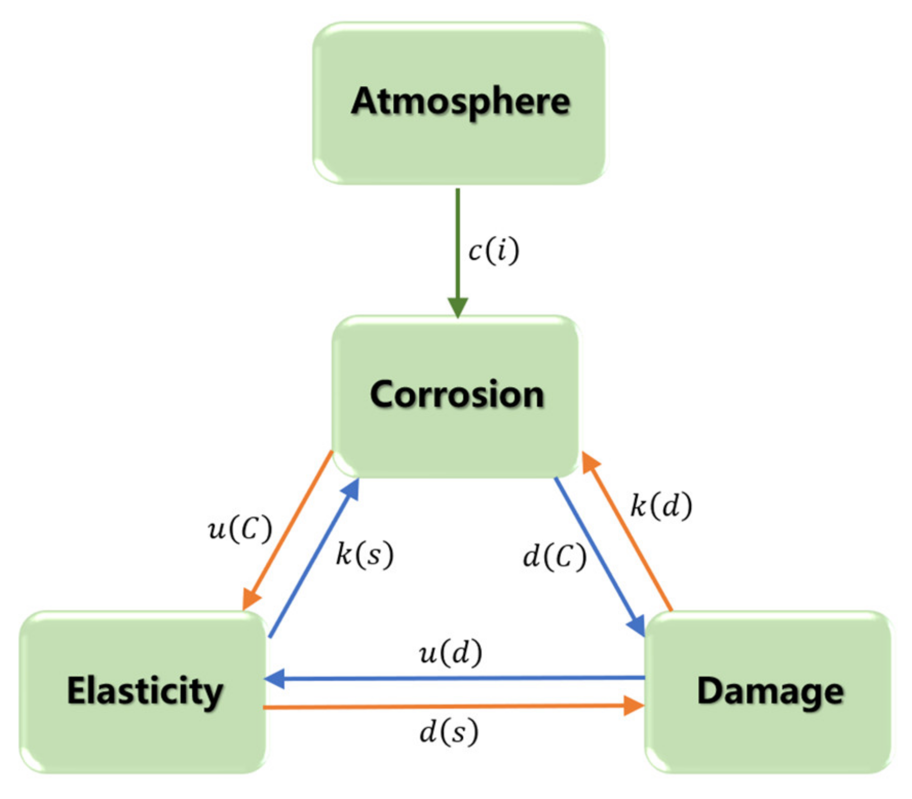
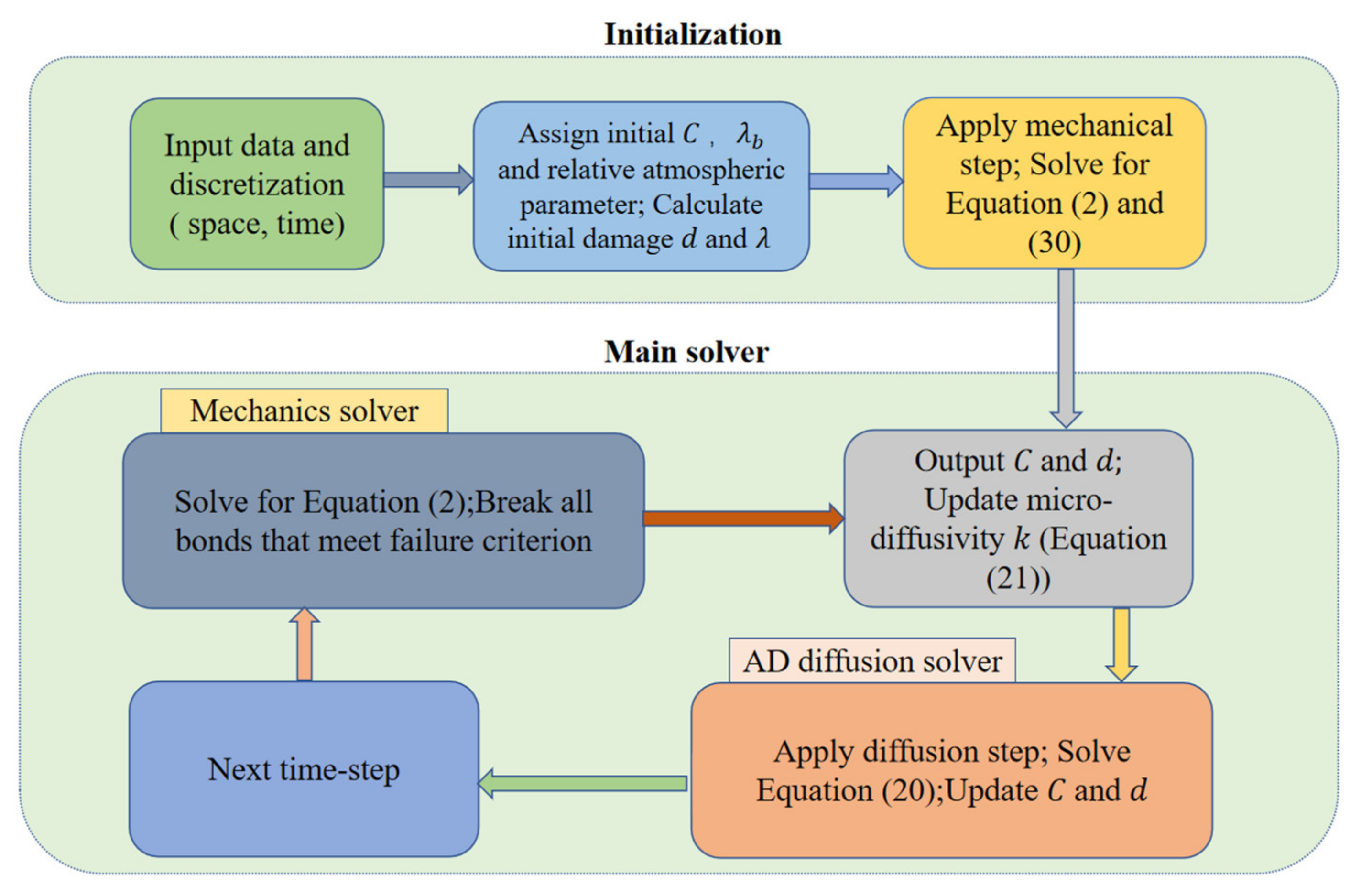
2.1.4. Atmospheric Corrosion–Fracture Coupling Model with Peridynamics

In this part, the mechano-chemical coupled kinetic model for near-field kinetic ASCC is introduced. In the previous sections, the PD fracture model, the air corrosion process, and the anodic dissolution model were covered briefly. In the fracture model, the nodes carry information about the displacement ( u ) and mechanical strain damage index ( d s ); in the atmospheric corrosion mechanism, they carry information about the liquid film thickness ( λ ) and corrosion mechanism ( c i ); and in the anodic dissolution model, they carry information about the concentration ( C ) and corrosion damage index ( d c ). Figure 3 illustrates the links between them.
Starting from the top of the figure, environmental changes lead to changes in the electrolyte film thickness, where the film thickness is updated according to Equation (15) and the corrosion mechanism is determined according to Equation (26). Starting from the corrosion evolution and moving in a clockwise direction: electrochemical corrosion leads to a phase change in the corrosion front of the metal according to Equation (23); then, the corrosion damage index is updated, the displacement and bond strain are updated according to Equation (2) under the current load, and finally, the microsolubility is updated according to Equation (30). In the counterclockwise direction: alterations in the corrosion process’s progression lead to the distribution of metal displacement under a mechanical force, and when the bond stretch exceeds the critical bond strain, mechanical damage occurs, and according to the corrosion damage connection in Equation (21), the cumulative mechanical damage accelerates corrosion.
We numerically simulated atmospheric stress corrosion cracking using the algorithm shown in Figure 4. It refers to the algorithm reported by Siavash Jafarzadeh et al. [36]. There were two main differences: the hydrogen atoms were involved in the anodic dissolution type of SCC and atmospheric stress corrosion cracking was formulated through the thickness variation of the electrolyte liquid film.
Solution steps: The region in the defined material was discretized with a uniform grid and the relevant parameters were entered for modeling. The initial concentration C, the initial liquid film base thickness λ b , the relevant atmospheric parameters were set, and the initial damage d and the initial liquid film thickness λ were calculated. Equation (1) was solved using the mechanics solver step and k d i s s s was found using Equation (30). For the AD diffusion solver: the diffusion of metal ions at each time step was solved using the near-field kinetic diffusion model (Equation (20)), and the concentration C and the damage index d of the metal ions were updated. For the mechanics solver: when the metal ion diffusion step cycle was completed, the displacement of the material point was solved using Equation (1) and the damage d at the material point was updated.

2.2. Simulation of Atmospheric Stress Corrosion Fracturing in 304 Stainless Steel
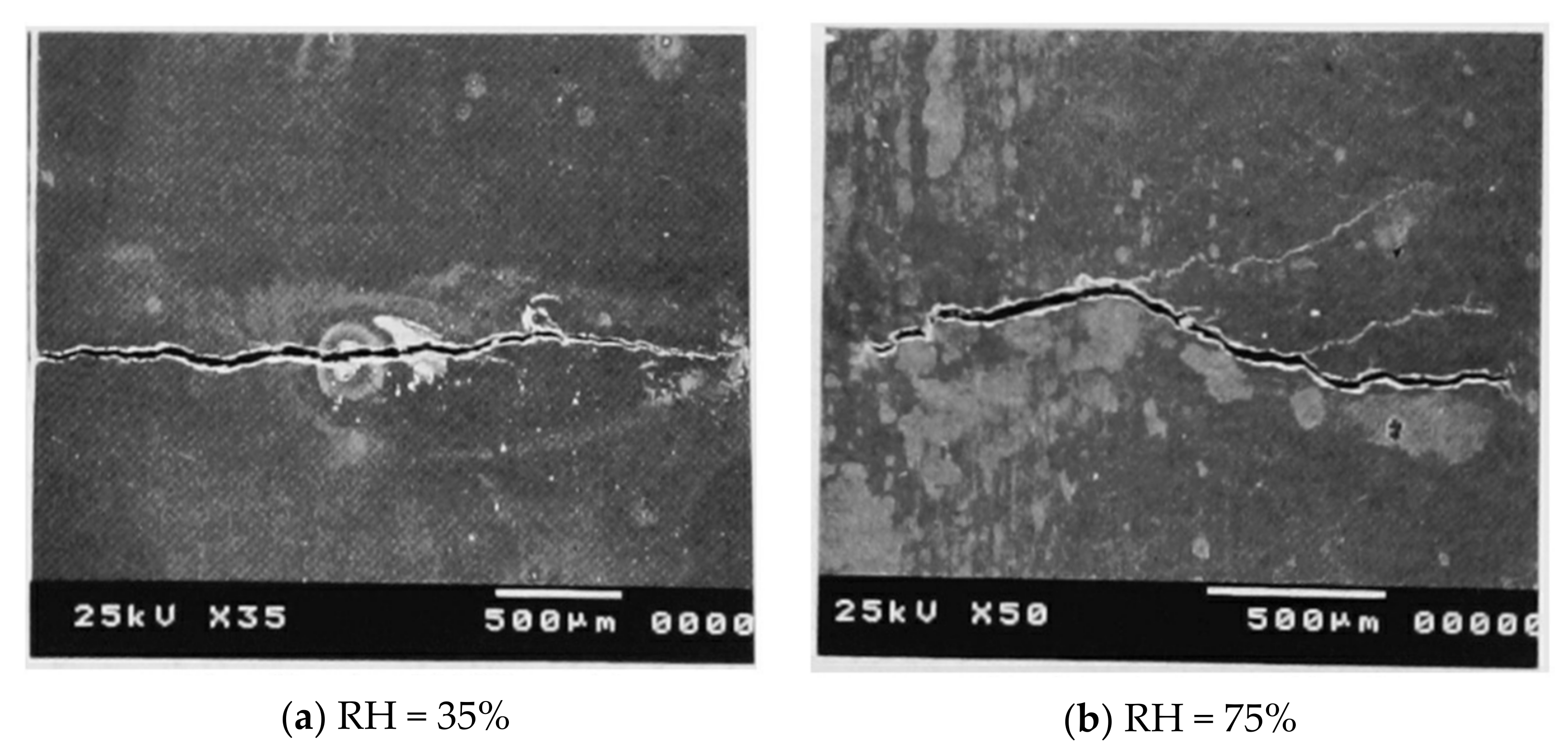
In this section, we discuss the 3D simulations of the atmospheric corrosion of 304 stainless steel under controlled laboratory conditions using a coupled near-field kinetic atmospheric corrosion–fracture model in which artificial seawater was used, where stress corrosion of 304 stainless steel in an acidic chloride ion atmosphere is widely believed to be dominated by anodic dissolution, with the participation of hydrogen atoms in promoted anodic dissolution corrosion of the metal [54,55].

2.2.1. Experiment

To verify whether the coupled near-field kinetic atmospheric corrosion–fracture model proposed above could capture the crack extension of the atmospheric corrosion of 304 stainless steel, we compared the experimental results with the numerically simulated crack extension results.
Masami Mayuzumi et al. [56] placed 304 stainless steel in a laboratory at constant temperature (353 K) with adjustable humidity and dripped 30μLto 50μL of M g C l 2 artificial seawater on the surface of the specimen, applied a constant load during the experiment, and investigated the morphology of crack extension of the specimen at 35% relative humidity and 75% relative humidity (Figure 5).
Figure 5 shows the scanning electron micrographs of corrosion cracks on the specimen surface. The main purpose of this study was to investigate the crack expansion in atmospheric stress corrosion, and it was reasonable to prefabricate the cracks in the simulation experiments in order to simplify the model and improve the computational efficiency.
The chemical composition of 304 stainless steel is shown in Table 1.

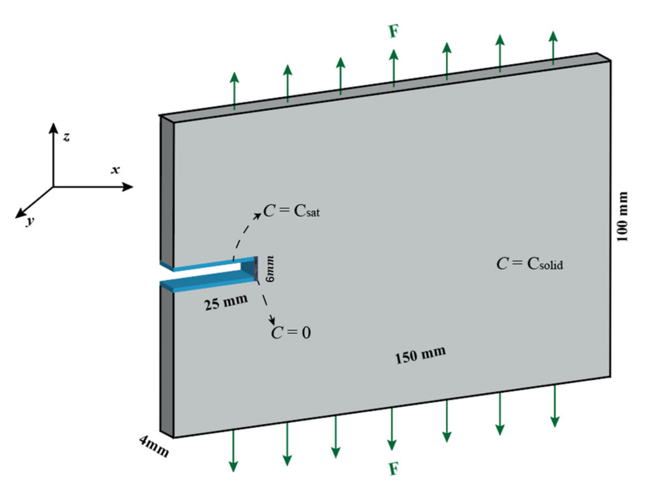
2.2.2. Calculation Model Setup

To simplify the model and improve the computational efficiency, we set the numerical simulation model as a rectangular plate of 150 × 4 × 100   mm 3 . As shown in Figure 6, the initial crack length was 25 mm and a constant load was applied at the top and bottom edges of the plate. A layer of nodes to the right of the initial crack was used as the initial corrosion area, and the metal ion concentration in the initial corrosion area was set to zero and maintained at zero throughout the corrosion process. Zero-flux conditions were applied to the rest of the boundaries. The region describing the material was discretized using a uniform grid with nodes situated in the center of each cell, which was equivalent to employing Gaussian quadrature with a single point in the vicinity.
The region defining the material was discretized with a uniform grid with the nodes located in the middle of each cell, which was equivalent to using a single-point Gaussian quadrature in the neighborhood.
The computational model consisted of 60,000 material points of 1   m m size, with eight particle layers at the bottom and top edges as loading layers, with a grid spacing Δ x = 1   m m and a near-field radius δ = 3   mm (corresponding to m = 3), which was uniformly discretized in the x , y , and z directions with Δ x . The Young’s modulus of 304 stainless steel E = 194020   MPa and the Poisson’s ratio v = 0.3 ; we chose C s o l i d = 143   M , C s a t = 5.1   M , and λ 0 = 30   μ m , which are typical values for stainless steel, and applied C s a t at the location of the crack tip and along the newly created crack node. We assumed that the solubility of the corrosion front was 0.02   μ m 2 / s , and to improve the modeling rate, by referring to the calculation in [57], we used k H = 1.07 , k σ = 1.001 , and k H , σ = 1.08 . Typically, the plastic deformation of steel must be accounted for in the fracture model. However, as the plasticity of stainless steel decreases in corrosive environments, the ductile fracture transforms into a quasi-brittle fracture, necessitating the use of the intrinsic force model of brittle material with linear and nonlinear mechanical behavior in the solution process.
In the process of stress corrosion, the time for corrosion diffusion is much longer than the time for crack expansion; therefore, the time t for corrosion diffusion calculation in the computational model should be much larger than the time T for the mechanical solution step. Moreover, the given initial liquid film thickness λ B has a great influence on the results of the numerical simulation. Therefore, we conducted experiments to determine the appropriate time interval and initial liquid film thickness in the following section.

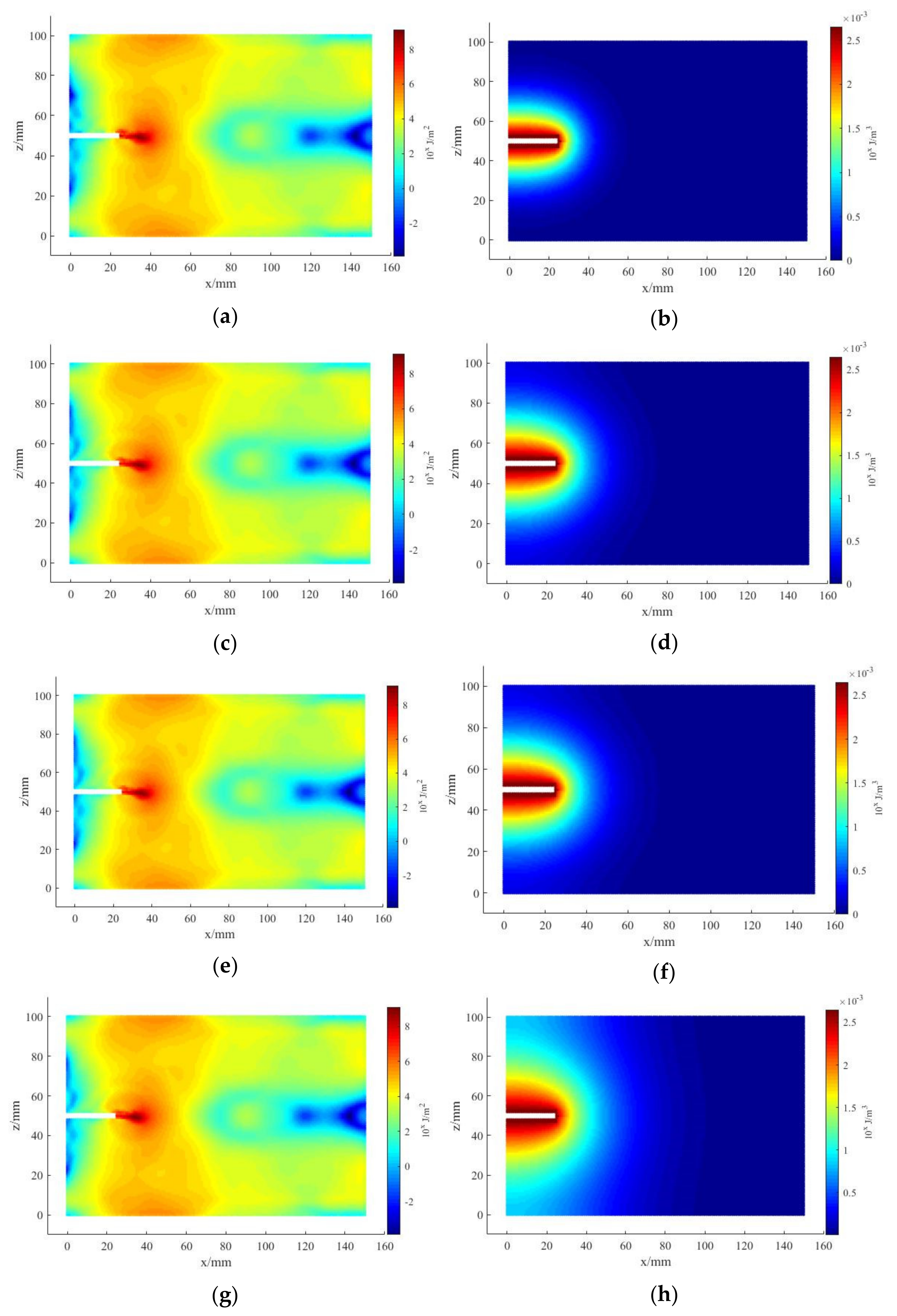
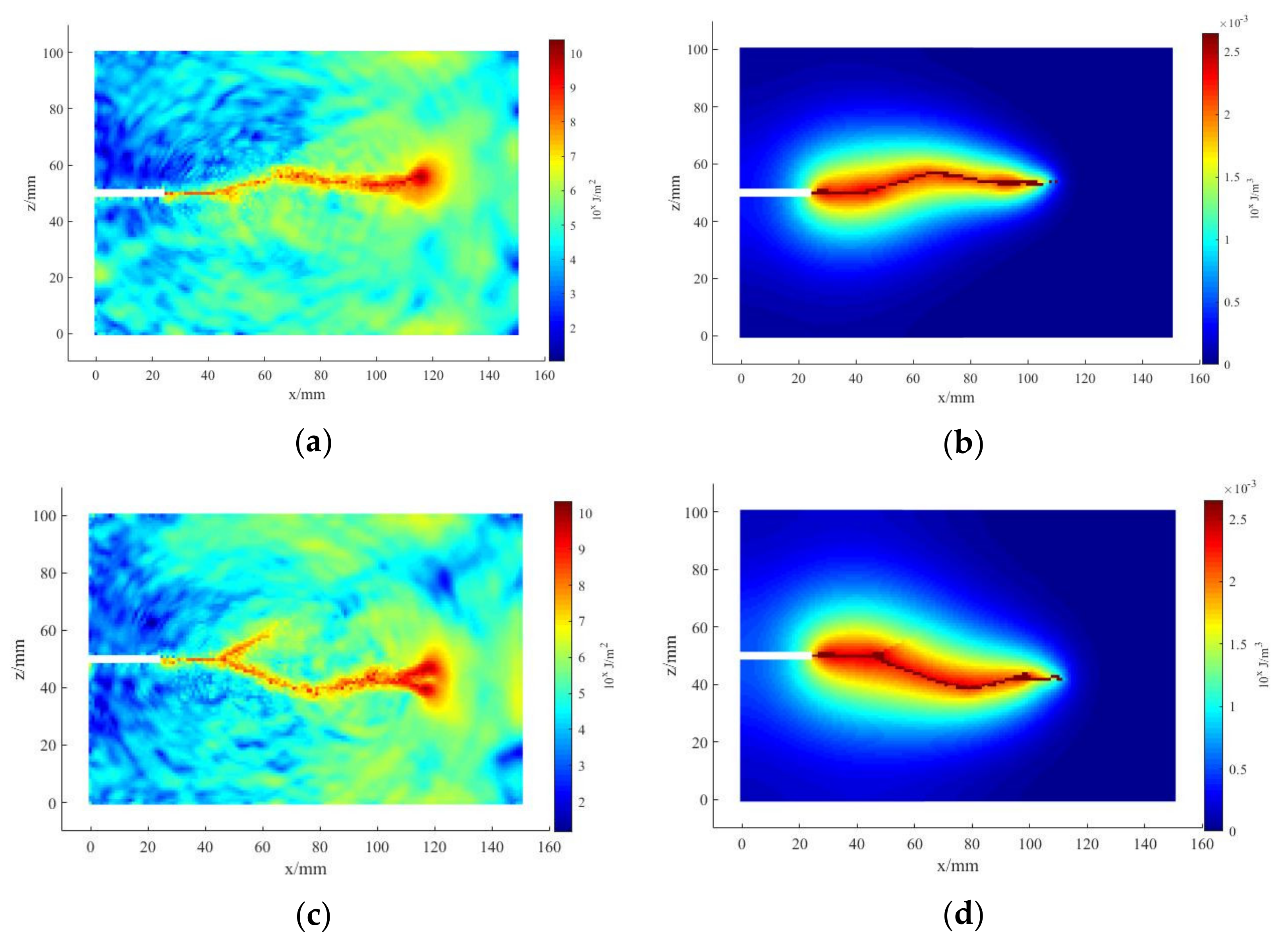
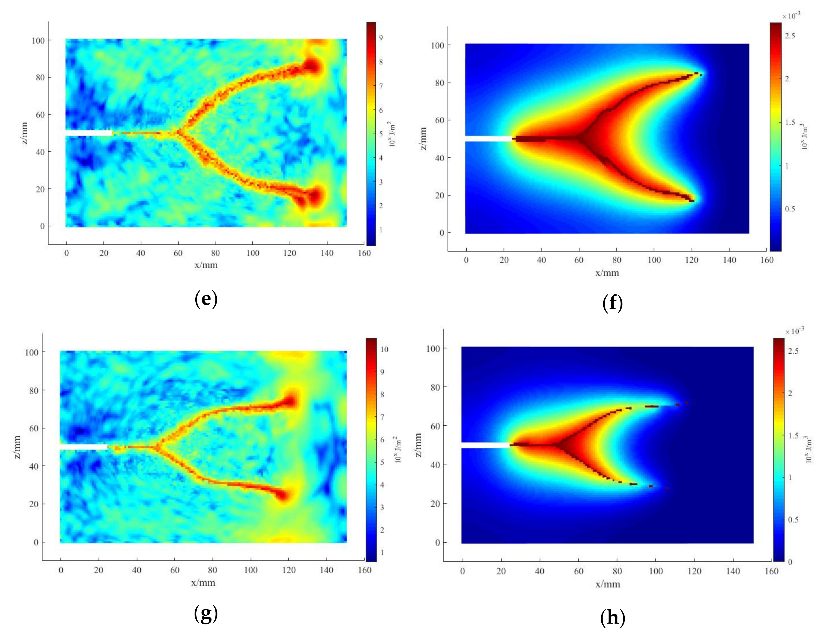
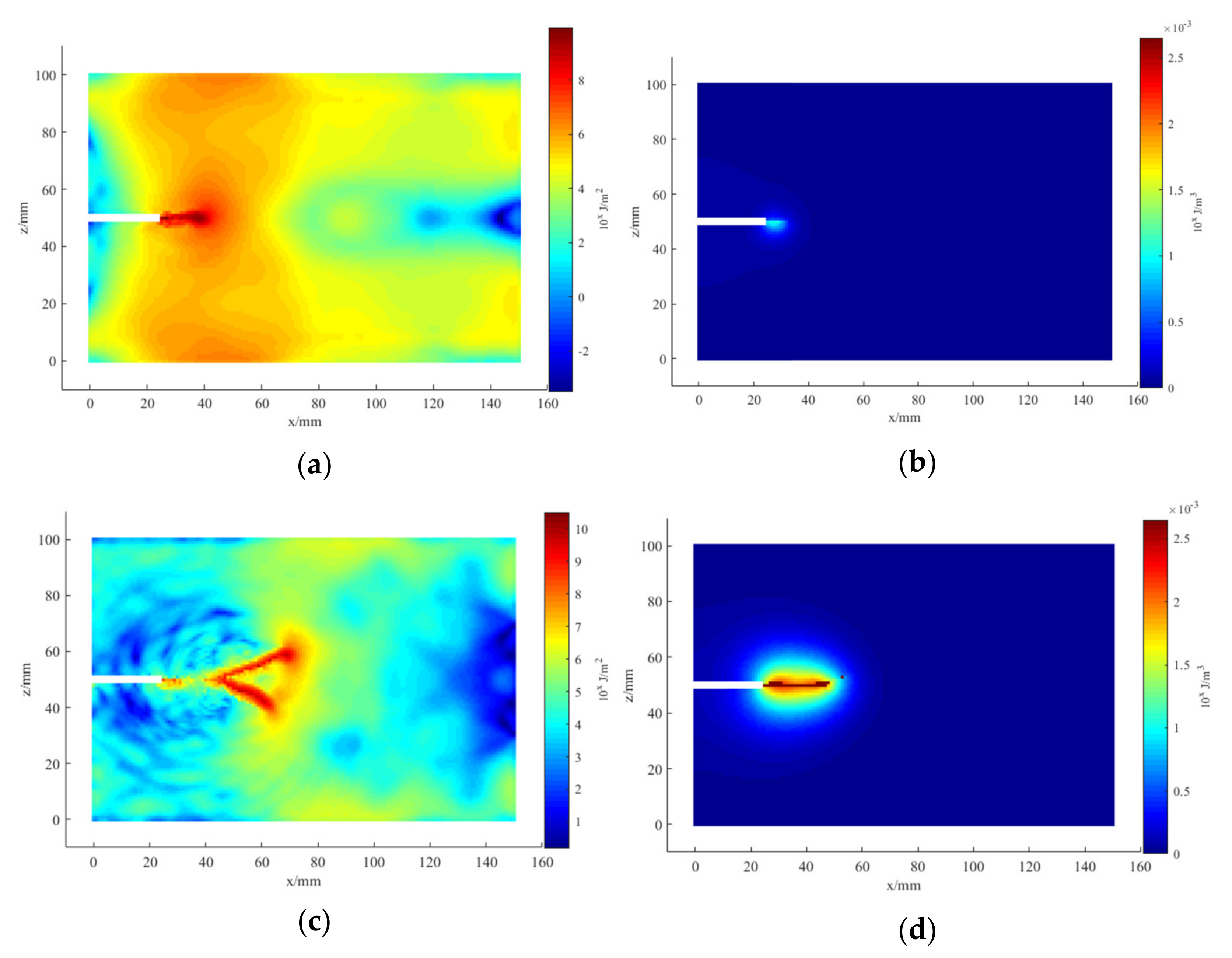
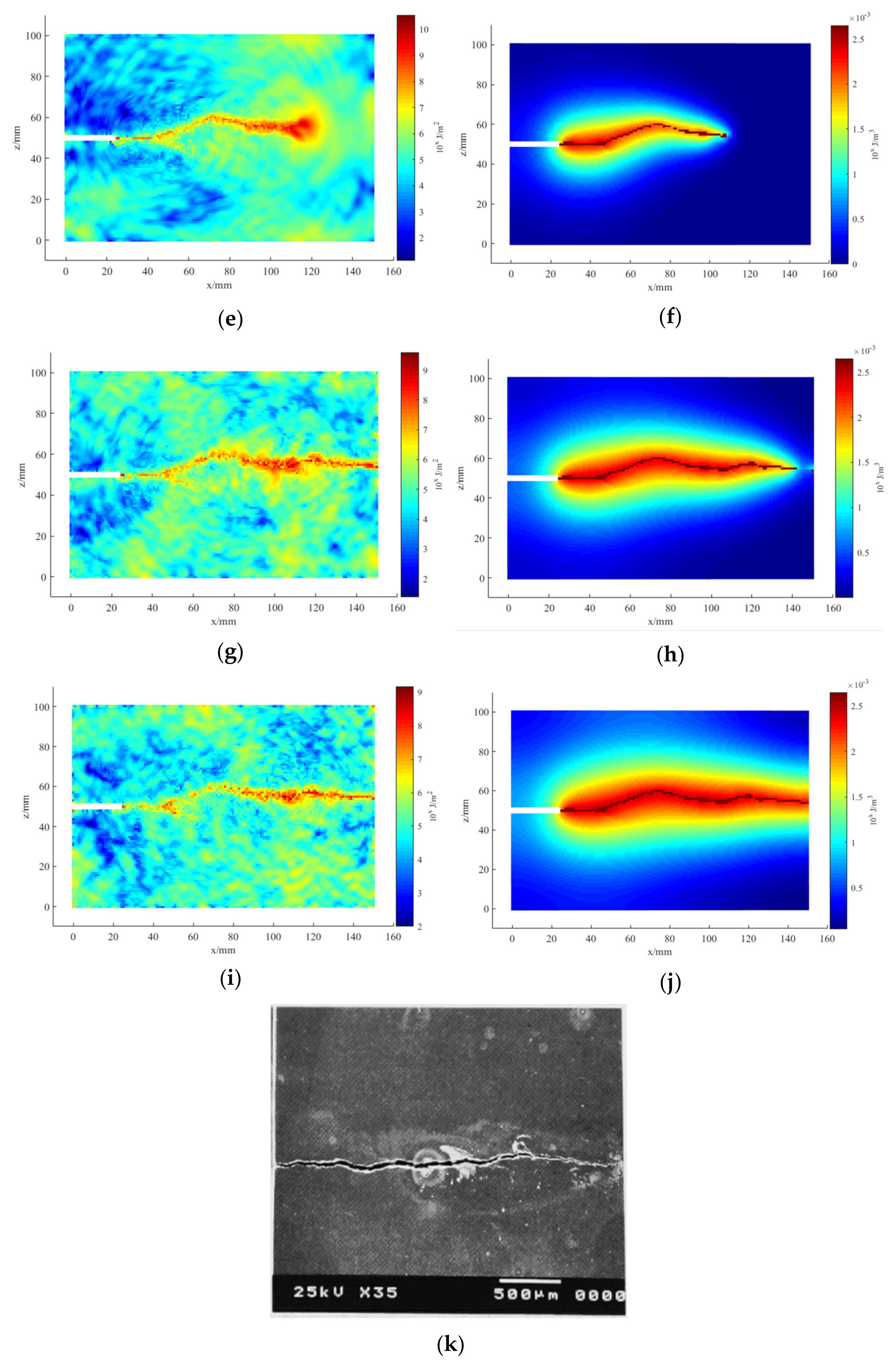
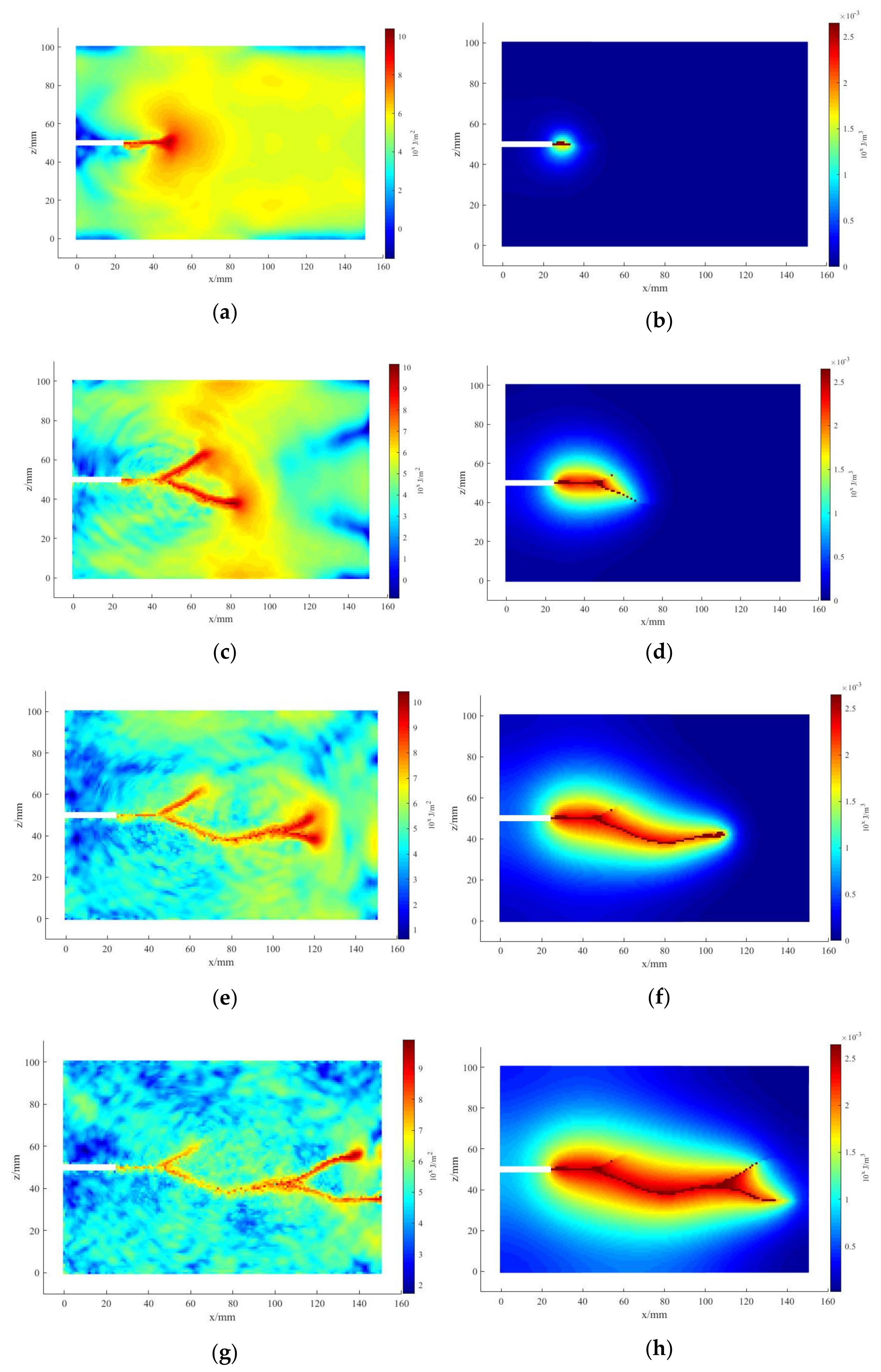
3. Results and Discussion

In order to study the effect of the corrosion diffusion time t with mechanical loading time T and the initial liquid film thickness on the numerical simulation of the stress corrosion process, we performed the simulation solution based on the data model with RH = 35% relative humidity under the condition that all the boundaries were not set to zero flux. We first studied the effect of the corrosion diffusion time t and mechanical loading time T . Four sets of simulations were done: T = 30t (40t, 50t, 60t) when t = 30 (40, 50, 60), i.e., the corrosion diffusion solver ran 30 (40, 50, 60) time steps after the fracture solver ran once. The results are shown in Figure 7. The red-brown part of the energy sketch (left) indicates the mechanical damage release energy. The red-brown part of the corrosion diffusion domain diagram (right) corresponds to the region where the metal ion concentration in the metal matrix became zero.
Figure 7 shows that in the case of a coupled solver with the same running time, the longer the corrosion diffusion solver ran, the greater the corroded region. The direction of fracture expansion was toward the region of corrosion diffusion in this investigation.
Taking λ B = 0.5   μ m   5   μ m ,   50   μ m ,   500   μ m , T = 40 t , setting the initial corrosion region metal ion concentration to zero, and applying zero flux to the rest of the boundary, we did four sets of simulation experiments to determine the effect of the initial electrolyte film thickness, and the simulation results are shown in Figure 8. As shown in Figure 8: As λ B becomes larger, the area of corrosion diffusion also becomes larger, and is accompanied by the appearance of branching cracks. When λ B to increase to a certain extent, the same time step under the area of corrosion diffusion in turn becomes smaller. This is in line with the effect of electrolyte film thickness on corrosion rate.
Lu et al. [58] demonstrated that oxygen plays a key role in the nucleation and extension of stress corrosion cracks. For IGSCC cracks, oxidation first occurs before the SCC crack tip. The crack then expands by connecting with microcracks within the grain interface oxide. For TGSCC cracks, the nucleation and growth of microcracks in the oxide along the deformation zone is an important mechanism for TGSCC crack extension. This was consistent with the partially discontinuous cracks in Figure 8b,d,f,h in the simulation experiments, further justifying the model.
Through simulation experiments, we found that the thickness of the electrolyte liquid film not only affected the rate of stress corrosion to a great extent but also affected the sprouting and evolution of branching cracks during the stress corrosion process. Through the above two simulation experiments, we found that the selection of the appropriate time interval and the initial liquid film thickness had an important influence on the simulation solution.
Based on the above simulation experiments, the metal ion concentration in the initial corrosion region was set to zero and zero flux was applied to the boundary of the remaining prefabricated cracks. We used T = 40 t and λ B = 0.5   μ m and numerically simulated the atmospheric stress corrosion of 304 stainless steel in a laboratory environment with a relative humidity RH of 35%. We used T = 40 t and λ B = 5   μ m and numerically simulated the atmospheric stress corrosion of 304 stainless steel in a laboratory environment with a relative humidity RH of 75%. The results are shown in Figure 9 and Figure 10. We found that the results of the numerical simulation of the model and the experimental results displayed good agreement. Both were dominated by transverse cracks and had some similarities in the direction of branching cracks.
Nyrkova et al. [5], through the study of stress corrosion of X70 pipeline steel in a near-neutral environment, found that the stress corrosion process can proceed both according to the anodic dissolution mechanism and according to the hydrogen embrittlement mechanism. 304 stainless steel samples due to local anodic dissolution on the surface formed the initial corrosion areas, these initial corrosion areas are the original defects of crack generation. In these defect areas, will cause a large stress concentration. At the same time, the hydrogen atoms generated during the anodic dissolution process will be enriched in the stress concentration area, and the hydrogen atoms will diffuse through the defects to the metal interior under the effect of concentration gradient and stress gradient.
Chiari et al. [59], through a positron annihilation lifetime spectroscopy study on 304 stainless steel, confirmed that hydrogen diffuses into a deeper region after the application of tensile stress. Simultaneously, vacant hydrogen complexes are generated in this region and develop into vacant clusters. This study corroborated the role of hydrogen and stress in anodic-dissolution-dominated SCC.
Haruna et al. [60] studied the stress corrosion of iron-containing chloride ion rust layers that occurred in humidity-controlled air. The results of the study showed that the relative humidity affected the rate of hydrogen uptake by the rust layer of iron. In the region of 42–74% RH, the hydrogen uptake rate increased with increasing RH. The pH of the rust layer was weakly acidic in the range of 4.2–4.3 during the corrosion in the tested RH range. Therefore, the higher the relative humidity within the range of 42–74%, the more hydrogen the metal absorbed during the stress corrosion. The greater the stress gradient and concentration gradient (hydrogen diffusion in metal mainly occurs via stress diffusion), the greater the diffusion range of hydrogen atoms in the metal. Under tensile stress, the direction of the crack extension remained essentially the same as the direction of diffusion of hydrogen atoms. This was highly similar to our simulation tests.
Chengshuang Zhou et al. [61], in their study of X80 pipeline steel hydrogen embrittlement, found that when hydrogen embrittlement occurs in this material, the hydrogen originated from internal hydrogen and surface-absorbed hydrogen. When the material was charged with hydrogen, hydrogen atoms were first adsorbed on the metal surface, and then hydrogen penetrated the metal and became internal hydrogen. When the hydrogen charging was stopped, the absorbed hydrogen on the surface disappeared and the internal hydrogen atoms diffused outward. We set the boundary conditions with zero concentration of hydrogen atoms outside the model, i.e., only hydrogen atoms existed inside the model. In this case, the diffusion direction of hydrogen should be toward the right outer boundary of the model under the stress gradient and concentration gradient. In Figure 9 and Figure 10, the results of our numerical simulations were consistent with the hydrogen atom diffusion law of Chengshuang Zhou et al. [61], which showed that our model was reasonable.

4. Conclusions

In this study, a coupled model of atmospheric stress corrosion was proposed, which was based on the near-field kinetic theory, near-field kinetic anodic dissolution theory, and atmospheric corrosion theory. In the near-field kinetic anodic dissolution theory, the factors of hydrogen, stress, and the hydrogen and stress synergy are added to express the role of hydrogen and stress in stress corrosion that is dominated by anodic dissolution. It should be noted that in our model, the role of hydrogen atoms was to promote the anodic dissolution of the metal rather than to produce hydrogen embrittlement. In the theory of atmospheric corrosion, the influence of the thickness of the electrolyte liquid film on the rate and mechanism of atmospheric corrosion is the main consideration. The variation in the liquid film thickness was calculated using the main factors that affect the variation of liquid film thickness. Then, a coupled near-field kinetic anodic dissolution and atmospheric corrosion model was proposed. This coupled model enabled the numerical simulation of stress corrosion of metals that occur in an atmospheric environment.
We used the atmospheric stress corrosion of 304 stainless steel as a control experiment. In the simulation experiments, it was found that ASCC cracks started to sprout from the prefabricated cracks and expanded toward the boundary of the sample under the combined effect of stress and hydrogen atoms, and the relative humidity had an important effect on the rate and direction of crack expansion. Within a certain relative humidity range (35–75%), the increase in relative humidity accelerated the corrosion rate. The results of the numerical simulations were in good agreement with the experimental results.
Because our model simplified the role of hydrogen and stress in the anodic dissolution process, it did not consider the influence of the material microstructure, and the calculation of the liquid film thickness was relatively simple in the atmospheric corrosion model. Therefore, the numerical simulation results had some errors relative to the experimental results.

Author Contributions

Conceptualization, Formal analysis and Writing—original draft, C.T.; Funding acquisition, Resources, S.Q.; Software, J.Z. All authors have read and agreed to the published version of the manuscript.

Funding

Guizhou Optoelectronic Information and Intelligent Application International Joint ReSearch Center (Qiankehe Platform Talents No.5802[2019]).

Institutional Review Board Statement

Not applicable.

Informed Consent Statement

Not applicable.

Data Availability Statement

Not applicable.

Acknowledgments

The authors gratefully acknowledge the financial support from the Guizhou International Science and Technology Cooperation Base Project.

Conflicts of Interest

The authors declare no conflict of interest.

References

  1. Hansson, C.M. The Impact of Corrosion on Society. Met. Mater. Trans. A 2011, 42, 2952–2962. [Google Scholar] [CrossRef]
  2. Koushik, B.G.; Steen, N.V.D.; Mamme, M.H.; Van Ingelgem, Y.; Terryn, H. Review on modelling of corrosion under droplet electrolyte for predicting atmospheric corrosion rate. J. Mater. Sci. Technol. 2020, 62, 254–267. [Google Scholar] [CrossRef]
  3. Ramamurthy, S.; Atrens, A. Stress corrosion cracking of high-strength steels. Corros. Rev. 2013, 31, 1–31. [Google Scholar] [CrossRef] [Green Version]
  4. Flanagan, W.; Bastias, P.; Lichter, B. A theory of transgranular stress-corrosion cracking. Acta Met. et Mater. 1991, 39, 695–705. [Google Scholar] [CrossRef]
  5. Lu, Y.; Peng, Q.; Sato, T.; Shoji, T. An ATEM study of oxidation behavior of SCC crack tips in 304L stainless steel in high temperature oxygenated water. J. Nucl. Mater. 2005, 347, 52–68. [Google Scholar] [CrossRef]
  6. Dadfarnia, M.; Martin, M.L.; Nagao, A.; Sofronis, P.; Robertson, I.M. Modeling hydrogen transport by dislocations. J. Mech. Phys. Solids 2015, 78, 511–525. [Google Scholar] [CrossRef]
  7. Jiang, D.; Carter, E.A. First principles assessment of ideal fracture energies of materials with mobile impurities: Implications for hydrogen embrittlement of metals. Acta Mater. 2004, 52, 4801–4807. [Google Scholar] [CrossRef]
  8. Barnoush, A.; Asgari, M.; Johnsen, R. Resolving the hydrogen effect on dislocation nucleation and mobility by electrochemical nanoindentation. Scr. Mater. 2012, 66, 414–417. [Google Scholar] [CrossRef]
  9. Lynch, S. Hydrogen embrittlement phenomena and mechanisms. Corros. Rev. 2012, 30, 105–123. [Google Scholar] [CrossRef]
  10. Leyson, G.; Grabowski, B.; Neugebauer, J. Multiscale description of dislocation induced nano-hydrides. Acta Mater. 2015, 89, 50–59. [Google Scholar] [CrossRef]
  11. Schindelholz, E.; Kelly, R.G. Wetting phenomena and time of wetness in atmospheric corrosion: A review. Corros. Rev. 2012, 30, 135–170. [Google Scholar] [CrossRef]
  12. Simillion, H.; Dolgikh, O.; Terryn, H.; Deconinck, J. Atmospheric corrosion modeling. Corros. Rev. 2014, 32, 73–100. [Google Scholar] [CrossRef]
  13. Steen, N.V.D.; Simillion, H.; Dolgikh, O.; Terryn, H.; Deconinck, J. An integrated modeling approach for atmospheric corrosion in presence of a varying electrolyte film. Electrochim. Acta 2016, 187, 714–723. [Google Scholar] [CrossRef]
  14. Stratmann, M.; Streckel, H. The Investigation of the Corrosion of Metal Surfaces, Covered with Thin Electrolyte Layers—A New Experimental Technique. Ber. Der Bunsenges. Für Phys. Chem. 1988, 92, 1244–1250. [Google Scholar] [CrossRef]
  15. Nishikata, A.; Ichihara, Y.; Tsuru, T. Electrochemical impedance spectroscopy of metals covered with a thin electrolyte layer. Electrochim. Acta 1996, 41, 1057–1062. [Google Scholar] [CrossRef]
  16. Nishikata, A.; Ichihara, Y.; Hayashi, Y.; Tsuru, T. Influence of Electrolyte Layer Thickness and pH on the Initial Stage of the Atmospheric Corrosion of Iron. J. Electrochem. Soc. 1997, 144, 1244–1252. [Google Scholar] [CrossRef]
  17. Liu, Z.; Wang, W.; Wang, J.; Peng, X.; Wang, Y.; Zhang, P.; Wang, H.; Gao, C. Study of corrosion behavior of carbon steel under seawater film using the wire beam electrode method. Corros. Sci. 2014, 80, 523–527. [Google Scholar] [CrossRef]
  18. Shi, Y.; Tada, E.; Nishikata, A. A Method for Determining the Corrosion Rate of a Metal under a Thin Electrolyte Film. J. Electrochem. Soc. 2015, 162, C135–C139. [Google Scholar] [CrossRef]
  19. Chung, K.-W.; Kim, K.-B. A study of the effect of concentration build-up of electrolyte on the atmospheric corrosion of carbon steel during drying. Corros. Sci. 2000, 42, 517–531. [Google Scholar] [CrossRef]
  20. Ito, M.; Ooi, A.; Tada, E.; Nishikata, A. In Situ Evaluation of Carbon Steel Corrosion under Salt Spray Test by Electrochemical Impedance Spectroscopy. J. Electrochem. Soc. 2020, 167, 101508. [Google Scholar] [CrossRef]
  21. Saeedikhani, M.; Steen, N.V.D.; Wijesinghe, S.; Vafakhah, S.; Terryn, H.; Blackwood, D.J. Moving Boundary Simulation of Iron-Zinc Sacrificial Corrosion under Dynamic Electrolyte Thickness Based on Real-Time Monitoring Data. J. Electrochem. Soc. 2020, 167, 041503. [Google Scholar] [CrossRef]
  22. Simillion, H.; Steen, N.V.D.; Terryn, H.; Deconinck, J. Geometry influence on corrosion in dynamic thin film electrolytes. Electrochim. Acta 2016, 209, 149–158. [Google Scholar] [CrossRef]
  23. Gupta, D.; Eom, H.-J.; Cho, H.-R.; Ro, C.-U. Hygroscopic behavior of NaCl–MgCl2 mixture particles as nascent sea-spray aerosol surrogates and observation of efflorescence during humidification. Atmospheric Chem. Phys. 2015, 15, 11273–11290. [Google Scholar] [CrossRef] [Green Version]
  24. Schindelholz, E.; Risteen, B.E.; Kelly, R.G. Effect of Relative Humidity on Corrosion of Steel under Sea Salt Aerosol Proxies. J. Electrochem. Soc. 2014, 161, C460–C470. [Google Scholar] [CrossRef]
  25. Cole, I.; Ganther, W.D.; Sinclair, J.D.; Lau, D.; Paterson, D.A. A Study of the Wetting of Metal Surfaces in Order to Understand the Processes Controlling Atmospheric Corrosion. J. Electrochem. Soc. 2004, 151, B627–B635. [Google Scholar] [CrossRef]
  26. Cole, I.; Azmat, N.S.; Kanta, A.; Venkatraman, M. What really controls the atmospheric corrosion of zinc? Effect of marine aerosols on atmospheric corrosion of zinc. Int. Mater. Rev. 2009, 54, 117–133. [Google Scholar] [CrossRef]
  27. Cole, I.; Paterson, D.A. Modelling aerosol deposition rates on aircraft and implications for pollutant accumulation and corrosion. Corros. Eng. Sci. Technol. 2009, 44, 332–339. [Google Scholar] [CrossRef]
  28. Belytschko, T.; Black, T. Elastic crack growth in finite elements with minimal remeshing. Int. J. Numer. Meth. Eng. 1999, 45, 601–620. [Google Scholar] [CrossRef]
  29. Schlangen, E.; van Mier, J.G.M. Simple lattice model for numerical simulation of fracture of concrete materials and structures. Mater. Struct. 1992, 25, 534–542. [Google Scholar] [CrossRef]
  30. Silling, S. Reformulation of elasticity theory for discontinuities and long-range forces. J. Mech. Phys. Solids 2000, 48, 175–209. [Google Scholar] [CrossRef]
  31. De Meo, D.; Diyaroglu, C.; Zhu, N.; Oterkus, E.; Siddiq, M.A. Modelling of stress-corrosion cracking by using peridynamics. Int. J. Hydrogen Energy 2016, 41, 6593–6609. [Google Scholar] [CrossRef] [Green Version]
  32. Madenci, E.; Yaghoobi, A.; Barut, A.; Phan, N. Peridynamic Modeling of Compression after Impact Damage in Composite Laminates. J. Peridynamics Nonlocal Model. 2021, 3, 327–347. [Google Scholar] [CrossRef]
  33. Jafarzadeh, S.; Chen, Z.; Bobaru, F. Peridynamic Modeling of Repassivation in Pitting Corrosion of Stainless Steel. Corrosion 2017, 74, 393–414. [Google Scholar] [CrossRef]
  34. Jafarzadeh, S.; Chen, Z.; Bobaru, F. Peridynamic Modeling of Intergranular Corrosion Damage. J. Electrochem. Soc. 2018, 165, C362–C374. [Google Scholar] [CrossRef]
  35. Chen, Z.; Zhang, G.; Bobaru, F. The Influence of Passive Film Damage on Pitting Corrosion. J. Electrochem. Soc. 2015, 163, C19–C24. [Google Scholar] [CrossRef]
  36. Jafarzadeh, S.; Chen, Z.; Li, S.; Bobaru, F. A peridynamic mechano-chemical damage model for stress-assisted corrosion. Electrochim. Acta 2019, 323, 134795. [Google Scholar] [CrossRef]
  37. Chen, Z.; Jafarzadeh, S.; Zhao, J.; Bobaru, F. A coupled mechano-chemical peridynamic model for pit-to-crack transition in stress-corrosion cracking. J. Mech. Phys. Solids 2020, 146, 104203. [Google Scholar] [CrossRef]
  38. Ran, X.; Qian, S.; Zhou, J.; Xu, Z. Crack propagation analysis of hydrogen embrittlement based on peridynamics. Int. J. Hydrogen Energy 2021, 47, 9045–9057. [Google Scholar] [CrossRef]
  39. Li, Y.; Liu, Z.; Wu, W.; Li, X.; Zhao, J. Crack growth behaviour of E690 steel in artificial seawater with various pH values. Corros. Sci. 2019, 164, 108336. [Google Scholar] [CrossRef]
  40. Gong, K.; Wu, M.; Xie, F.; Liu, G.; Sun, D. Effect of Cl− and rust layer on stress corrosion cracking behavior of X100 steel base metal and heat-affected zone in marine alternating wet/dry environment. Mater. Chem. Phys. 2021, 270, 124826. [Google Scholar] [CrossRef]
  41. Gong, K.; Wu, M.; Liu, G. Stress corrosion cracking behavior of rusted X100 steel under the combined action of Cl− and HSO3− in a wet–dry cycle environment. Corros. Sci. 2020, 165, 108382. [Google Scholar] [CrossRef]
  42. Chen, W.; Hao, L.; Dong, J.; Ke, W. Effect of sulphur dioxide on the corrosion of a low alloy steel in simulated coastal industrial atmosphere. Corros. Sci. 2014, 83, 155–163. [Google Scholar] [CrossRef]
  43. Hu, Y.; Dong, C.; Sun, M.; Xiao, K.; Zhong, P.; Li, X. Effects of solution pH and Cl− on electrochemical behaviour of an Aermet100 ultra-high strength steel in acidic environments. Corros. Sci. 2011, 53, 4159–4165. [Google Scholar] [CrossRef]
  44. Ives, M.; Lu, Y.; Luo, J. Cathodic reactions involved in metallic corrosion in chlorinated saline environments. Corros. Sci. 1991, 32, 91–102. [Google Scholar] [CrossRef]
  45. Liu, Z.; Du, C.; Zhang, X.; Wang, F.; Li, X. Effect of pH value on stress corrosion cracking of X70 pipeline steel in acidic soil environment. Acta Met. Sin. (English Lett.) 2013, 26, 489–496. [Google Scholar] [CrossRef] [Green Version]
  46. Guo, X.; Gao, K.; Qiao, L.; Chu, W. The correspondence between susceptibility to SCC of brass and corrosion-induced tensile stress with various pH values. Corros. Sci. 2002, 44, 2367–2378. [Google Scholar] [CrossRef]
  47. Lu, Q.; Wang, L.; Xin, J.; Tian, H.; Wang, X.; Cui, Z. Corrosion evolution and stress corrosion cracking of E690 steel for marine construction in artificial seawater under potentiostatic anodic polarization. Constr. Build. Mater. 2019, 238, 117763. [Google Scholar] [CrossRef]
  48. Katona, R.; Carpenter, J.; Knight, A.; Bryan, C.; Schaller, R.; Kelly, R.; Schindelholz, E. Importance of the hydrogen evolution reaction in magnesium chloride solutions on stainless steel. Corros. Sci. 2020, 177, 108935. [Google Scholar] [CrossRef]
  49. Madenci, E.; Oterkus, E. Peridynamic Theory and Its Applications; Springer: Berlin/Heidelberg, Germany, 2014. [Google Scholar] [CrossRef]
  50. Silling, S.; Askari, E. A meshfree method based on the peridynamic model of solid mechanics. Comput. Struct. 2005, 83, 1526–1535. [Google Scholar] [CrossRef]
  51. Wang, J.; Qian, S. Spallation Analysis of Concrete Under Pulse Load Based on Peridynamic Theory. Wirel. Pers. Commun. 2020, 112, 949–966. [Google Scholar] [CrossRef]
  52. Bobaru, F.; Duangpanya, M. The peridynamic formulation for transient heat conduction. Int. J. Heat Mass Transf. 2010, 53, 4047–4059. [Google Scholar] [CrossRef]
  53. Bobaru, F.; Duangpanya, M. A peridynamic formulation for transient heat conduction in bodies with evolving discontinuities. J. Comput. Phys. 2012, 231, 2764–2785. [Google Scholar] [CrossRef] [Green Version]
  54. Krishnan, K.; Rao, K.P. Effect of microstructure on stress corrosion cracking behaviour of austenitic stainless steel weld metals. Mater. Sci. Eng. A 1991, 142, 79–85. [Google Scholar] [CrossRef]
  55. Qiao, L.; Mao, X. Thermodynamic analysis on the role of hydrogen in anodic stress corrosion cracking. Acta Met. Mater. 1995, 43, 4001–4006. [Google Scholar] [CrossRef]
  56. Mayuzumi, M.; Arai, T.; Hide, K. Chloride Induced Stress Corrosion Cracking of Type 304 and 304L Stainless Steels in Air. Zairyo-to-Kankyo 2003, 52, 166–170. [Google Scholar] [CrossRef]
  57. Qiao, L.; Mao, X.; Chu, W. The role of hydrogen in stress-corrosion cracking of austenitic stainless steel in hot MgCl2 solution. Met. Mater. Trans. A 1995, 26, 1777–1784. [Google Scholar] [CrossRef]
  58. Nyrkova, L.; Melnichuk, S.; Osadchuk, S.; Lisovyi, P.; Prokopchuk, S. Investigating the mechanism of stress corrosion cracking of controllable rolling pipe steel X70 in near-neutral environment. Mater. Today Proc. 2021, 50, 470–476. [Google Scholar] [CrossRef]
  59. Chiari, L.; Komatsu, A.; Fujinami, M. Defects Responsible for Hydrogen Embrittlement in Austenitic Stainless Steel 304 by Positron Annihilation Lifetime Spectroscopy. ISIJ Int. 2021, 61, 1927–1934. [Google Scholar] [CrossRef]
  60. Haruna, T.; Shoji, Y.; Hirohata, Y. Hydrogen Absorption Rate into Fe with Rust Layer Containing NaCl during Atmospheric Corrosion in Humidity-controlled Air. ISIJ Int. 2021, 61, 1079–1084. [Google Scholar] [CrossRef]
  61. Zhou, C.; Ye, B.; Song, Y.; Cui, T.; Xu, P.; Zhang, L. Effects of internal hydrogen and surface-absorbed hydrogen on the hydrogen embrittlement of X80 pipeline steel. Int. J. Hydrogen Energy 2019, 44, 22547–22558. [Google Scholar] [CrossRef]
Figure 1. The peridynamic analysis of the movement of matter points.
Applsci 12 10008 g001
Figure 2. The relationship between the force density vector f and the elongation S .
Applsci 12 10008 g002
Figure 3. Schematic of the coupled peridynamic atmosphere corrosion–fracture model.
Applsci 12 10008 g003
Figure 4. Graphical illustration of the coupled peridynamic atmosphere corrosion–fracture model.
Applsci 12 10008 g004
Figure 5. SEM image of the sample surface.
Applsci 12 10008 g005
Figure 6. Geometry and boundary conditions.
Applsci 12 10008 g006
Figure 7. Energy diagram ((a) T = 30 t , (c) T = 40 t , (e) T = 50 t , and (g) T = 60 t ) and corrosion diffusion field ((b) T = 30 t , (d) T = 40 t , (f) T = 50 t , and (h) T = 60 t ) in the 500-time-step test.
Applsci 12 10008 g007
Figure 8. Energy diagram ((a) λ B = 0.5   μ m , (c) λ B = 5   μ m , (e) λ B = 50   μ m , and (g) λ B = 500   μ m ) and crack propagation path ((b) λ B = 0.5   μ m , (d) λ B = 5   μ m , (f) λ B = 50   μ m , and (h) λ B = 500   μ m ) in the liquid film thickness test at 1200 time steps.
Applsci 12 10008 g008aApplsci 12 10008 g008b
Figure 9. Energy diagram ((a) t = 400 , (c) t = 800 , (e) t = 1200 , (g) t = 1600 , and (i) t = 2000 ), crack propagation path ((b) t = 400 , (d) t = 800 , (f) t = 1200 , (h) t = 1600 , and (j) t = 2000 ), and an SEM image of the sample surface (k) when the RH was 35%, with T = 40 t and λ B = 0.5   μ m .
Applsci 12 10008 g009aApplsci 12 10008 g009b
Figure 10. Energy diagram ((a) t = 400 , (c) t = 800 , (e) t = 1200 , (g) t = 1600 , and (i) t = 2000 ), crack propagation path ((b) t = 400 , (d) t = 800 , (e) t = 1200 , (h) t = 1600 , and (j) t = 2000 ), and an SEM image of the sample surface (k) when the RH was 75%, with T = 40 t and λ B = 0.5   μ m .
Applsci 12 10008 g010aApplsci 12 10008 g010b
Table 1. Chemical composition of the specimen.
CSiMnPSNiCrFe
0.06%0.61%0.95%0.028%0.011%8.12%18.10%Bal.
Publisher’s Note: MDPI stays neutral with regard to jurisdictional claims in published maps and institutional affiliations.

