Abstract
In the present paper, a new approach to identifying an arbitrary number of inclusions, their geometry and their location in 2D and 3D structures using topological optimization was proposed. The new approach was based on the lack of initial information about the geometry of the inclusions and their location in the structure. The numerical solutions were obtained by the finite element method in combination with the method of moving asymptotes. The convergence of the finite element method at the coincidence of functions and their derivatives was analyzed. Results with an error of no more than 0.5%, i.e., almost exact solutions, were obtained. Identification at impact on the plate temperature and heat flux by solving the inverse problem of heat conduction was produced. Topological optimization for identifying an arbitrary number of inclusions, their geometry and their location in 2D problems was investigated.
1. Introduction
Static and dynamic loads, as well as the wear process of a structure, can cause various types of structural damage. Damage, such as cracks and pores, causes a decrease in the mass and stiffness of mechanical structures, resulting in changes in their properties the latter being the main cause of failure in structural systems. This can be avoided by prior identification of damage present in the structure, and the service life of the structure can be extended by repairing the damages in time. In recent years, special attention has been given to methods that can detect damage at an early stage. Gomez et al. [1] proposed the use of inverse problems as a basic strategy for damage detection and identification in Structural Health Monitoring (SHM). Das et al. [2] presented an efficient multi-stage optimization damage detection method for truss and frame structures equipped with a limited number of sensors. In this approach, a Finite Element (FE) model was developed to simulate the response of the actual structure. De Assis et al. [3] applied metaheuristic sunflower optimization, the artificial neural networks and the response surface method to solve the inverse problem of crack identification. The crack was modeled as a thin elliptical hole in a rectangular layered plate using the finite element method. The methods yielded various approaches to solve the problem, and provided reliable identification of the shape, size and position of a crack ranging in size from 3 to 30 mm. Hatlas et al. [4] conducted multi-scale global identification. To solve the identification problem, task global optimization methods (evolutionary algorithm), finite element method commercial software, the response surface approach and the numerical homogenization algorithm were combined. Lee et al. [5] used eigenfrequency sensitivity analysis to detect defects in beams. The effectiveness of the boundary element method (BEM) was compared with that of the finite element method (FEM). Vinh et al. [6] analyzed the static bending and buckling of bi-directional, functionally graded (BFG) plates with porosity using a new, first-order shear deformation theory (FSDT) based on the mixed finite element method (FEM). Cuong-Le et al. [7] studied the linear and nonlinear solutions of a sigmoid functional-gradient nanoplate (S-FGM) with porous effects. Numerical size-dependent solutions were obtained using strain gradient theory and an isogeometric finite-element formulation.
Please note that the application of the FEM and the BEM is one of the effective approaches for solving the direct problem and detecting structural damage. The inverse problem of determining the location and size of the damage was modeled using methods such as: (1) methods based on artificial neural networks [8,9,10,11,12]; (2) multiple loading methods [13,14,15,16] and (3) methods based on topological optimization approaches [17,18,19,20,21,22,23,24]. The topological derivative representing the sensitivity for an arbitrary shape, which is functional with respect to the generation of an infinitesimal singular domain perturbation, such as inclusion, was introduced by Sokołowski et al. [17], and its development was found [18]. Kefal et al. [19] developed a robust and accurate approach based on the innovative coupling of peridynamics (PD) (a meshless method) and topology optimization (TO) to determine the optimum topology of load-bearing structures. Park [20] considered the topological derivative in a limited-aperture inverse scattering problem for noniterative imaging of thin inhomogeneity. Wahab et al. [21] established a topological sensitivity framework for far field detection of diametrically small electromagnetic inclusions. Pena et al. [22] studied the use of steady and time-harmonic thermograms for structural health monitoring of thin plates. The Topological-Shape Sensitivity Method in various fields of technology, including shape and topology optimization [23], inverse problems [24] and damage development modeling [25], has been used. Fernandez et al. [26,27] used the topological derivative method to solve a pollution sources reconstruction problem governed by a steady-state convection–diffusion equation. Xue et al. [28] applied the contingent probability method to track sources of pollutants in open air with a constant emission. Da Silva et al. [29] proposed a new approach to the problem of damage identification in plate structures based on the method of topological derivatives. Three inclusions were identified with 32% confidence. Wei et al. [30] developed an approach based on an improved particle swarm optimization (PSO) algorithm for damage detection in structures. Khatir et al. [31] applied extended isogeometric analysis (X-IGA) combined with PSO for crack identification in two-dimensional linear elastic problems based on the inverse problem. Pereira et al. [32] developed numerical identification and characterization of damage propagation using a new optimization technique called Lichtenberg optimization (LA). Fathi et al. [33] presented a new geometry-based crack detection approach for plate structures based on the integration of the dynamic extended finite element method (XFEM) and an optimization algorithm called the enhanced vibrating particle system (EVPS). Hassine et al. [34] focused on the detection of objects immersed in an anisotropic medium by boundary measurements. A one-iteration algorithm based on the Kona-Vogelius formulation and the topological gradient method was proposed. The inverse problem was formulated as a topological optimization approach. Machado et al. [35] proposed rewriting the inverse source problem as an optimization problem, where the functional Con-Vogelius type was minimized with respect to the set of admissible point sources. Goncalves et al. [36] considered the identification of acoustic parameters in the frequency domain using a topological problem optimization approach. Pena et al. [37] applied active time-harmonic infrared thermography to detect defects inside of thin plates. Burchinski et al. [38] reviewed bioinspired methods for solving various inverse problems for mechanical systems. Abda et al. [39] proposed an approach based on the so-called energy-like error functional, in combination with the topological sensitivity method. The topological derivative of the energy-like error functional was calculated using the topological shape sensitivity method. Numerical tests to indicate the effectiveness of the developed approach were performed. Krysko et al. [40,41,42,43] proposed the application of topological optimization methods based on temperature and heat flux measurements. The effects on the optimal topology of the composite in the presence of two competing materials were investigated, in addition to the optimality criteria, using linear weight functions. Pareto spaces were constructed, providing an in-depth understanding of how these goals compete to achieve optimal topology. The problem of topological optimization of multilayer structural elements of MEMS/NEMS resonators with an adhesive layer under the action of mechanical loads was also considered. The problems of the finite element method were solved using the method of sliding asymptotes.
According to the author’s knowledge, and as summarized in the above review, the application of topological optimization methods for the identification of holes/inclusions is still finite. The available publications are devoted to the identification of single holes/ inclusions of the simplest geometry (ellipse and circle), and the quality of the identification work described is not acceptable. Therefore, the main aim of this work was to develop a new approach to identifying an arbitrary number of inclusions, their geometries and locations in 2D and 3D structures, with high recognition quality. Numerical solutions were obtained using the FEM in conjunction with the sliding asymptote method. Damage identification is the first step in the investigations of the stress–strain state (SSS) and stability of mechanical structures, followed by the study of the SSS and stability of perforated mechanical structures [44] with already-known inclusion locations, determined by TO.
The work is organized as follows. Section 2 describes a new approach to the determination of an arbitrary number of inclusions, their geometry and their location in the structure by means of topological optimization. Then, Section 3 discusses the obtained numerical results, and Section 4 presents the concluding remarks on the results of this study.
2. Materials and Methods
A new approach to identifying an arbitrary number of inclusions, their geometry and their location in 2D and 3D structures was based on the influence of temperature and heat flux on the structure. This solves the inverse heat conduction problem.
Consider an isotropic flat cuboid body (Figure 1), inside which there are inclusions occupying the area V1, V2, … Vm, m = 1, 2 ….
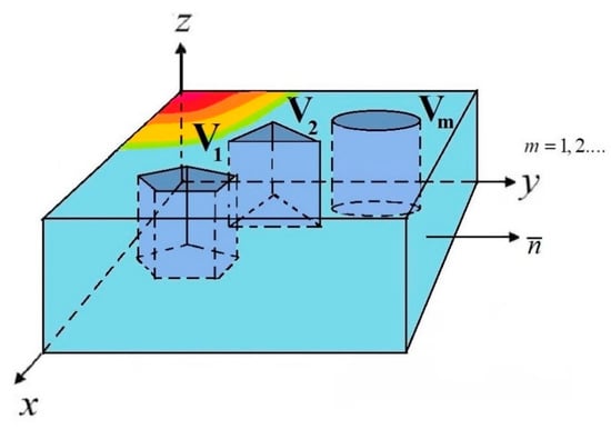
Figure 1.
The cuboid isotropic flat body with selected areas .
The body was under the action of both the temperature at the boundary BT (the Dirichlet (or first type) boundary condition) and the heat flux at the boundary Bq (the Neumann (or second type) boundary condition). The temperature field T inside V satisfies the heat conduction equation [40]
and boundary conditions
where , T0 is the set temperature at BT; q0 is the heat flux determined on Bq; n—is the unit normal vector directed outward of the area. In the area of V defined subdomains V1, V2, …, Vm with the coefficient of thermal conductivity k1, k2, …, km.
To form the topological optimization procedure, the area was divided into finite elements. Then, each element was assigned a variable density, which depends on the vector of design variables . The thermal conductivity coefficient depends on the artificially introduced density , which will be the control variable when using the Solid Isotropic Material with Penalty method (SIMP) [45].
The thermal conductivity coefficient was introduced as follows:
where —are thermal conductivity coefficients in volumes , respectively, and is a penalty factor for the SIMP method. The goal function was defined as follows [40]:
where the first term is the penalty function to eliminate the “checkerboard” effect; is the coefficient for matching the target function and the penalty function; represents the initial grid size; is the current grid size; is the area of the inclusions; is the physical density; is the temperature on a flat area and is calculated temperature on a flat area; is a given flow on an area and is the calculated flow on a flat area.
Limitations for physical density are chosen as the following:
where denotes the fraction of material in the inclusions. Identification consists of minimizing the difference in temperature distribution and heat fluxes in the original design, and obtaining them in this iteration step.
3. Numeric Experiments and Results Discussion
We intend to examine some examples of challenges of identifying an arbitrary number and planning inclusions, their geometry and their location in a plate, under the influence of temperature and thermal flows, using topological optimization. Let us consider an isotropic flat body in the form of a thin plate occupying the area , inside which are inclusions occupying the area , with the thermal conductivity coefficients (Figure 2).
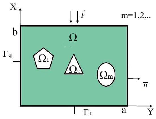
Figure 2.
Plate design with marked areas ,
, … .
We write the classical differential heat equation [40] for the temperature field T inside the area Ω
and boundary conditions
where is the given temperature at ; is the heat flux, installed on the and is the vector of the normal to the boundary of the area. The equations were reduced to their dimensionless forms in the standard way [46]. Next, problems (7)–(9) were solved by the Finite Element Method using the COMSOL Multiphysics software.
3.1. Problem 1: Investigating the Convergence of a Solution by the FEM Using the COMSOL Multiphysics Software
To obtain reliable results, the convergence of the solution by the finite element method was studied using the COMSOL Multiphysics software. The basic material of the plate in the area was steel, with the coefficient of thermal conductivity (CTC) , and —stood for inclusions of aluminum with the CTC . The reliability of the obtained results was considered achieved if the error did not exceed 0.5% of the previous solution. The study was carried out for three types of inclusions related to geometry (rectangle, rhombus, square), but the total number of inclusions was equal to 18. The obtained results are reported in Table 1.

Table 1.
The area Ω, divided into 18 rectangular inclusions, with corresponding coordinates of the inclusion center—problem 1.
Let us examine the partition into FE of 18 inclusions in the form of rectangles, which are located: vertically (Table 2), horizontally (Table 3) and at an angle of 45 degrees (Table 4). Let us also study the influence of location and geometry on the identification result. The tables are reported: the width of the rectangle; rectangle length; the number of FEs when splitting into a small grid and the number of FEs when splitting into a large grid. Each table presents data on the partition into finite elements for three similar cases, while gradually decreasing the width of the plate. The partitions are presented for two values of the size inclusion: (a) ; (b) .
Table 2.
Location of inclusions in the area and number of FEs for different size a.
Table 3.
Distribution of the thermal field and the result of identification of rectangular shapes. Inclusions (18 elements)—Problem 2; .
Table 4.
Distribution of the thermal field and identification results for rectangular-shaped inclusions (18 elements) rotated by 90 degrees—Problem 3; .
From the data presented in Table 2, several conclusions can be drawn: (1) The location of rectangular inclusions significantly effects the partition of the grid (, ); (2) size width is decreased—a, for rectangular inclusions, leads to an increase in the number of FE, and for , the increase is by more than 2 times.
3.2. Problem 2: Investigation of the Influence of the Boundary Conditions of the Thermal Problem on the Identification of a Large Number of Inclusions in the Form of Rectangles
In this example, the influence of three types of boundary conditions of the thermal problem on the identification of a large number of inclusions in the form of rectangles was considered. The following boundary conditions for the thermal problem (7) were used:
The results of the distribution of the thermal field and identification of inclusions for the different boundary conditions of the thermal Equation (7) are shown in Table 3.
Upon impact of heat flux only to the left boundary of the plate (boundary condition (10) (Table 3a)), the left column of inclusions was identified. Inclusions number 2 and 17 in the center column are incompletely identified (Table 3d). In the case of an impact of heat flux on the left and upper boundary of the plate (boundary condition (11), (Table 3b)), inclusions 17 and 18 were not completely identified (Table 3e). In the case when the heat fluxes impacted on the left, upper and lower boundaries of the plate (boundary condition (12), (Table 3c)), then all inclusions were identified (Table 3f). Thus, the use of the boundary condition (12) allows you to fully identify all inclusions. It can be concluded that these boundary conditions significantly affect the inclusion’s identification (Table 3f) and allow them to identify completely.
3.3. Problem 3: Investigation of the Influence of the Boundary Conditions of the Thermal Problem on the Identification of 18 Inclusions in the Form of Rectangles Rotated by 90 Degrees Compared to Problem 2
Table 4 shows the heat flux distribution, as well as the results of a study of the impact of the boundary conditions of the thermal problem on the identification of 18 rectangular shaped inclusions, rotated by 90 degrees compared to problem 2.
With impact of the heat flux only on the left boundary of the plate (boundary condition (10) (Table 4a)), the left and central columns are identified (Table 4d). In the case of impact of heat flux on the left and upper boundaries of the plate (boundary condition (11), (Table 4b)) inclusions 15, 17 and 18 (Table 4e) were not identified. In the case of heat flux impact on the left, upper and lower boundaries of the plate (boundary condition (12), (Table 4c)), all inclusions were identified (Table 4f). The results show that, as in the previous case (Table 3), when changing the direction of the inclusions. the best identification occurs when using the boundary condition (12).
3.4. Problem 4: Investigation of the Influence of the Boundary Conditions of the Thermal Problem on the Identification of 18 Inclusions in the Form of Rectangles Rotated by 45 Degrees Compared to Problem 3
Let us consider the case when the plate contains 18 rectangular-shaped inclusions rotated by 45 degrees, compared to problem 3.
Upon impact of heat flux only on the left border of the plate (boundary condition (10), (Table 5a)), the left and central columns were identified, except for two inclusions in column number 3 (Table 5d). In the case of impact of heat flux on the left and top plate boundary (boundary condition (11), (Table 5b)), inclusions 12, 15 and 18 (Table 5e) were not identified. In the case where heat flux impacted on the left, top and bottom of the plate (boundary condition (12), (Table 5c)), all inclusions were identified (Table 5f). The best identification occurred for the boundary condition (12), as well as for the examples given in Table 3 and Table 4. Based on the examples above, it should be concluded that the angle of rotation of rectangular inclusions relative to the Y-axis does not affect the identification of the boundary conditions (12).
Table 5.
Distribution of the thermal field and identification results for rectangular-shaped inclusions (18 elements) rotated by 45 degrees—Problem 4; .
3.5. Problem 5: Identification of the 18 Rhombuses Inclusions, under the Influence of Temperature and Heat Fluxes
Further, consider a problem with 18 inclusions in the shape of a rhombus with a side size of 0.05 m along the plate. The coordinates of the centers of these inclusions coincide with the coordinates of the rectangles (Table 1). The boundary conditions and the form of temperature and heat fluxes are the same as in Problem 2. The convergence of FEM when solving the direct problem of revealing of rhomboidal inclusions is presented in Table 6. The boundary conditions and the location of inclusions are presented in Table 7.
Table 6.
Investigation of convergence of FEM with different numbers of finite elements (FEs)—problem 5.
Table 7.
Distribution of the thermal field and the outcome of identification of rhomboidal inclusions (18 elements) with a side equal to 0.05 m—Problem 5.
The analysis of the obtained results (Table 6) shows that 1222 finite elements with an error = 0.5142% are sufficient to identify an area with 18 lozenge-like inclusions.
With the influence of heat flux only on the left border of the plate (boundary condition (10) (Table 7a)), identification occurred only for the left column of inclusions (Table 7d). A portion of the rhombuses, located in the 3rd column of the plate, was not identified. With the influence of heat flux on the left and top of the plate (boundary condition (11), (Table 7b)), unlike in the first case, almost all inclusions were identified except for the bottom one in the third column (Table 7e). In the case where heat flux influenced the left, bottom and top of the plate (boundary condition (12), (Table 7c)), almost all inclusions were identified (Table 7f). In Problems 2, 3 and 4, the best identification occurred for the boundary condition (12). It should be noted that changing the inclusions’ geometry does not have an effect on the identification process under the boundary condition (12).
3.6. Problem 6: Identification of the 18 Inclusions in the Form of a Square under the Influence of Temperature and Heat Fluxes
Let us consider the case when the plate contains 18 inclusions in the form of squares, each with a side size of 0.08 m. The coordinates of these inclusions are the same as the coordinates of the rectangles (Table 1). The boundary conditions and the form of temperature and heat fluxes are the same as in Problem 2. Investigation of the convergence of FEM to solve the direct problem of identifying inclusions in the form of squares were presented in Table 8. The boundary conditions and the location of inclusions were presented in Table 9.
Table 8.
Convergence and number of used finite elements (FEs)—problem 6.
Table 9.
Distribution of the thermal field and the outcome of identification of square inclusions (18 elements) with a side equal to 0.08 m—Problem 6.
Analysis of the results obtained (Table 8) showed that to identify an area with 18 square inclusions, 1330 finite elements are sufficient, with an error of = 0.5112%.
With the influence of the heat flux only on the left border of the plate (boundary condition ((10), (Table 9a)), not all inclusions are fully identified (Table 9d). This is due to the action of heat flux. It should be noted that the top and bottom inclusions are not fully identified. In the case when heat flux is applied to the left and upper boundaries of the plate (boundary condition (11), (Table 9b)), then the identification results (Table 9e) are better in contrast to Problem 2, but the upper and lower inclusions are also not completely identified. In the case when the heat flux is applied to the top, right and left boundaries of the plate (boundary condition (12), (Table 9c)), all inclusions are identified with good accuracy (Table 9f). An analysis of the results, which are presented in Table 3, Table 4, Table 5, Table 7 and Table 9, leads to the following conclusions. Under the action of the heat flux only on the left boundary of the plate (boundary condition (10), (Table 3a, Table 4a, Table 5a, Table 7a and Table 9a)) only the left column and the middle of the middle column were defined (Table 3d, Table 4d, Table 5d, Table 7d and Table 9d). It should be noted that the best identification result was obtained for small square inclusions; for rhombuses, it was slightly worse and for large square inclusions, identification was minimal. Thus, the type and size of the hole affects the process of determining the location and type of inclusions. In the case of action of the heat fluxes on the left and upper border of the plate (boundary condition (11), (Table 3b, Table 4b, Table 5b, Table 7b and Table 9b) parts of the inclusions in the lower rows were not defined (Table 3e, Table 4e, Table 5e, Table 7e and Table 9e). In the case when heat flux acted on the left, upper and lower boundaries of the plate (boundary condition (12), (Table 3f, Table 4f, Table 5f, Table 7f and Table 9f), then all inclusions were well-defined. As discussed in the above study, we can conclude that for all studies considered, the identification of all inclusions was fully achieved only when the heat flux was applied to three boundaries and boundary condition (12) was considered.
3.7. Problem 7: Identification of Inclusions by Changing Their Location, Number and Size
Let us consider the square plate containing inclusions in the form of rectangles with different types of arrangements (the data are presented in Table 10). For rectangles, two types of geometries were used, namely when the width, , decreases, and the value length, , does not change. The parameters for changing the width of the rectangles are shown in Table 10, in Roman numerals II and I. In addition, in Table 10, the distributions of heat flux for three cases of heat flux action, as well as boundary conditions (10)–(12), were presented.
Table 10.
Geometry, location of the inclusions and temperature distribution.
Identification results for cases I and II are presented in Table 11. However, one may also notice that, when the value of thickness (b) decreases, then the plate must be divided into a larger number of FEs. In this case, inclusions were identified with good accuracy. The heat flux was determined for three types of boundary conditions (10)–(12). It was found that for each variant of the boundary conditions, the identification results were different. This was especially noticeable in the case when the heat flux was specified from three sides of the plate and the boundary condition (12) was taken into account. Note that the size of the inclusions did not affect the quality of the identification.
Table 11.
Mesh configuration for inclusions in T-shape, and the results of identification for different boundary conditions.
Identification results and distribution of thermal fields for three «C» shaped rectangles are presented in Table 12. In order to obtain a good result for identifying narrower inclusions, the mesh was divided into a larger number of FEs than in the previous case. Afterwards, the inclusions were identified completely, especially in the case when the heat flux was supplied from three sides of the plate (boundary condition 12). Note that when the boundary conditions (10) and (11) were taken into account, the identification result was not of high quality. At the same time, for a “thin” inclusion, the identification under the boundary condition (11) was much better than for a “thick” inclusion, unlike the previous case.
Table 12.
Mesh configuration for inclusions in C-shape, and the results of identifications for different boundary conditions.
Identification results and distribution of thermal fields for three “H” -shaped rectangles are presented in Table 13. Inclusions took the shape we need, and were fully identified, when the heat flux was supplied from three sides, taking into account boundary conditions (12).
Table 13.
Mesh configuration for inclusions in H-shape and the result of identification for different boundary conditions.
For problem 7, for the identification of inclusions by changing their location, number and size, it can be concluded that when the boundary condition (12) was taken into account, the identification results did not depend on the location, number or size of inclusions.
4. Conclusions
This work discloses a new approach to identifying an arbitrary number of inclusions, their geometry and their location in 2D and 3D structures. This new approach is based on the use of topological optimization techniques, specifically the SIMP (Solid Isotropic Microstructure with Penalization for intermediate densities) method. The numerical solutions were obtained by the finite element method in combination with the method of moving asymptotes. Comsol Multiphysics software was used to simulate the constructed algorithm. Note that all previously known approaches are based on measuring the temperature and heat fluxes in the initial structure. This leads to the problem of determining the local thermal conductivity coefficient. The proposed approach is not affected by those constraints, and is applicable to the identification of any form of geometry or arrangement of inclusions in the three-dimensional problem of elasticity theory, as well as the two-dimensional problems of the theory of shells, plates and beams, and the plane problem of elasticity theory. According to the study presented herein, we can conclude that the newly developed approach is effective. In the present study, a large numerical experiment was conducted to determine the increase in the number of inclusions, their geometry and their location in the structure, which allowed us to draw the following conclusions:
- The best results for determining an arbitrary number of inclusions were obtained when taking into account heat flux from three sides of the boundary conditions (12). Note that, for boundary condition (12), the identification results are not affected by the location of the inclusion and its dimensions.
- The novelty of the proposed approach for inclusion identification allows us to neglect the initial information about the location of inclusions.
- Numerical results in the investigated problems were obtained “practically” as an exact solution. The calculation error does not exceed 0.5% of the exact one.
- The proposed approach and methodology for its implementation are the first step of the analysis of the stress–strain state of fracture of a structure during crack formation.
- A new approach for determining an arbitrary number of inclusions, their geometry and their location can be used to identify inclusions in 3D solids.
Author Contributions
Conceptualization, V.A.K.; data curation, M.V.Z. and A.M.; formal analysis, M.V.Z. and A.S.; funding acquisition, A.S.; investigation, A.V.K. and A.S.; methodology, V.A.K. and M.V.Z.; project administration, A.V.K.; resources, A.S. and V.A.K.; software, A.M.; supervision, V.A.K.; validation, A.V.K. and V.A.K.; visualization, A.M.; writing—original draft, V.A.K. and M.V.Z. All authors have read and agreed to the published version of the manuscript.
Funding
This work was supported by the Ministry of Science and Higher Education of the Russian Federation under project 0707-2020-0034.
Institutional Review Board Statement
Not applicable.
Informed Consent Statement
Not applicable.
Data Availability Statement
Not applicable.
Acknowledgments
This work was carried on the equipment of the Collective Use Center of MSTU “STANKIN” (project No. 075-15-2021-695).
Conflicts of Interest
The authors declare no conflict of interest.
References
- Gomes, G.F.; Mendez, Y.A.D.; Alexandrino, P.D.S.L.; da Cunha, S.S.; Ancelotti, A.C. A Review of Vibration Based Inverse Methods for Damage Detection and Identification in Mechanical Structures Using Optimization Algorithms and ANN. Arch. Comput. Methods Eng. 2019, 26, 883–897. [Google Scholar] [CrossRef]
- Das, S.; Dhang, N. Damage identification of structures using incomplete mode shape and improved TLBO-PSO with self-controlled multi-stage strategy. Structures 2022, 35, 1101–1124. [Google Scholar] [CrossRef]
- De Assis, F.M.; Gomes, G.F. Crack identification in laminated composites based on modal responses using metaheuristics, artificial neural networks and response surface method: A comparative study. Arch. Appl. Mech. 2021, 91, 4389–4408. [Google Scholar] [CrossRef]
- Hatłas, M.; Beluch, W. Multiscale global identification of porous structures. AIP Conf. Proc. 2018, 1922, 030005. [Google Scholar] [CrossRef]
- Lee, J. Boundary element method based sensitivity analysis of the crack detection in beams. J. Mech. Sci. Technol. 2015, 29, 3627–3634. [Google Scholar] [CrossRef]
- Van Vinh, P.; Van Chinh, N.; Tounsi, A. Static bending and buckling analysis of bi-directional functionally graded porous plates using an improved first-order shear deformation theory and FEM. Eur. J. Mech.-A Solids 2022, 96, 104743. [Google Scholar] [CrossRef]
- Cuong-Le, T.; Nguyen, K.D.; Le-M, H.; Phan-Vu, P.; Nguyen-Trong, P.; Tounsi, A. Nonlinear bending analysis of porous sigmoid FGM nanoplate via IGA and nonlocal strain gradient theory. Adv. Nano Res. 2022, 12, 441–455. [Google Scholar] [CrossRef]
- Mishra, M.; Barman, S.K.; Maity, D.; Maiti, D.K. Performance studies of 10 metaheuristic techniques in determination of damages for large-scale spatial trusses from changes in vibration responses. J. Comput. Civ. Eng. 2020, 34, 04019052. [Google Scholar] [CrossRef]
- Krishnanunni, C.G.; Raj, R.S.; Nandan, D.; Midhun, C.K.; Sajith, A.S.; Ameen, M. Sensitivity-based damage detection algorithm for structures using vibration data. J. Civ. Struct. Health Monit. 2019, 9, 137–151. [Google Scholar] [CrossRef]
- Huang, M.; Li, X.; Lei, Y.; Gu, J. Structural damage identification based on modal frequency strain energy assurance criterion and flexibility using enhanced Moth-Flame optimization. Structures 2020, 28, 1119–1136. [Google Scholar] [CrossRef]
- Sabokrou, M.; Fayyaz, M.; Fathy, M.; Moayed, Z.; Klette, R. Deep-anomaly: Fully convolutional neural network for fast anomaly detection in crowded scenes. Comput. Vis. Image Underst. 2018, 172, 88–97. [Google Scholar] [CrossRef]
- Gomes, G.F.; de Almeida, F.A. Tuning metaheuristic algorithms using mixture design: Application of sunflower optimization for structural damage identification. Adv. Eng. Softw. 2020, 149, 102877. [Google Scholar] [CrossRef]
- Liang, Y.-C.; Sun, Y.-P. Hardware-In-The-Loop Simulations of Hole/Crack Identification in a Composite Plate. Materials 2020, 13, 424. [Google Scholar] [CrossRef] [PubMed]
- Mei, H.; Haider, M.F.; Joseph, R.; Migot, A.; Giurgiutiu, V. Recent Advances in Piezoelectric Wafer Active Sensors for Structural Health Monitoring Applications. Sensors 2019, 19, 383. [Google Scholar] [CrossRef] [PubMed]
- Guemes, A. SHM of Composite structures by fiber optic sensors. In Structural Health Monitoring for Advanced Composite Structures, 1st ed.; Aliabadi, F.M.H., Khodaei, Z.S., Eds.; World Scientific Publishing Europe Ltd.: London, UK, 2018; Chapter 6; pp. 191–213. [Google Scholar] [CrossRef]
- Zhou, S.; Lin, H.; Li, B. Research on HILS Technology Applied on Aircraft Electric Braking System. J. Electr. Comput. Eng. 2017, 2017, 3503870. [Google Scholar] [CrossRef]
- Sokolowski, J.; Zochowski, A. On the topological derivative in shape optimization. SIAM J. Control Optim. 1999, 37, 1251–1272. [Google Scholar] [CrossRef]
- Novotny, A.A.; Sokołowski, J.; Żochowski, A. Studies in Systems, Decision and Control. In Applications of the Topological Derivative Method; Springer Nature Switzerland AG: Cham, Switzerland, 2019; 212p. [Google Scholar] [CrossRef]
- Kefal, A.; Sohouli, A.; Oterkus, E.; Yildiz, M.; Suleman, A. Topology optimization of cracked structures using peridynamics. Contin. Mech. Thermodyn. 2019, 31, 1645–1672. [Google Scholar] [CrossRef]
- Park, W.-K. Topological Derivative for Imaging of Thin Electromagnetic Inhomogeneity: Least Condition of Incident Directions. Adv. Math. Phys. 2018, 2018, 2096058. [Google Scholar] [CrossRef]
- Wahab, A.; Abbas, T.; Ahmed, N.; Zia, Q.M.Z. Detection of electromagnetic inclusions using topological sensitivity. J. Comp. Math. 2017, 35, 642–671. [Google Scholar] [CrossRef]
- Pena, M.; Rapún, M.-L. Detecting Damage in Thin Plates by Processing Infrared Thermographic Data with Topological Derivatives. Adv. Math. Phys. 2019, 2019, 5494795. [Google Scholar] [CrossRef]
- Nowak, M.; Sokołowski, J.; Żochowski, A. Justification of a certain algorithm for shape optimization in 3D elasticity. Struct. Multidiscip. Optim. 2018, 57, 721–734. [Google Scholar] [CrossRef]
- Ferreira, A.; Novotny, A.A. A new non-iterative reconstruction method for the electrical impedance tomography problem. Inverse Probl. 2017, 33, 035005. [Google Scholar] [CrossRef]
- Xavier, M.; Van Goethem, N.; Novotny, A.A. Hydro-mechanical fracture modeling governed by the topological derivatives. Comput. Methods Appl. Mech. Eng. 2020, 365, 112974. [Google Scholar] [CrossRef]
- Fernandez, L.; Novotny, A.A.; Prakash, R.; Sokołowski, J. Pollution Sources Reconstruction Based on the Topological Derivative Method. Appl. Math. Optim. 2021, 84, 1493–1525. [Google Scholar] [CrossRef]
- Fernández, L.; Novotny, A.A.; Prakash, R. Noniterative Reconstruction Method for an Inverse Potential Problem Modeled by a Modified Helmholtz Equation. Numer. Funct. Anal. Optim. 2018, 39, 937–966. [Google Scholar] [CrossRef]
- Xue, Y.; Zhai, Z.J. Inverse identification of multiple outdoor pollutant sources with a mobile sensor. Build. Simul. 2017, 10, 255–263. [Google Scholar] [CrossRef]
- Da Silva, A.A.M.; Novotny, A.A. Damage identification in plate structures based on the topological derivative method. Struct. Multidiscip. Optim. 2022, 65, 7. [Google Scholar] [CrossRef]
- Wei, Z.; Liu, J.; Lu, Z. Structural damage detection using improved particle swarm optimization. Inverse Probl. Sci. Eng. 2018, 26, 792–810. [Google Scholar] [CrossRef]
- Khatir, S.; Wahab, M.A.; Benaissa, B.; Köppen, M. Crack Identification Using eXtended IsoGeometric Analysis and Particle Swarm Optimization. In Lecture Notes in Mechanical Engineering, Proceedings of the 7th International Conference on Fracture Fatigue and Wear, Ghent, Belgium, 9–10 July 2018; Abdel Wahab, M., Ed.; Springer: Singapore, 2019. [Google Scholar] [CrossRef]
- Pereira, J.L.J.; Chuman, M.; Jr, S.S.C.; Gomes, G.F. Lichtenberg optimization algorithm applied to crack tip identification in thin plate-like structures. Eng. Comput. 2021, 38, 151–166. [Google Scholar] [CrossRef]
- Fathi, H.; Vaez, S.H.; Zhang, Q.; Alavi, A.H. A new approach for crack detection in plate structures using an integrated extended finite element and enhanced vibrating particles system optimization methods. Structures 2021, 29, 638–651. [Google Scholar] [CrossRef]
- Hassine, M.; Kallel, I. One-iteration reconstruction algorithm for geometric inverse problems. Appl. Math. E Notes 2018, 18, 43–50. [Google Scholar]
- Machado, T.J.; Angelo, J.S.; Novotny, A.A. A new one-shot pointwise source reconstruction method. Math. Methods Appl. Sci. 2017, 40, 1367–1381. [Google Scholar] [CrossRef]
- Gonçalves, J.F.; Moreira, J.B.D.; Salas, R.A.; Ghorbani, M.M.; Rubio, W.M.; Silva, E.C.N. Identification problem of acoustic media in the frequency domain based on the topology optimization method. Struct. Multidiscip. Optim. 2020, 62, 1041–1059. [Google Scholar] [CrossRef]
- Pena, M.; Rapún, M.L. Application of the topological derivative to post-processing infrared time-harmonic thermograms for defect detection. J. Math. Ind. 2020, 10, 4. [Google Scholar] [CrossRef]
- Burczyński, T.; Kuś, W.; Beluch, W.; Długosz, A.; Poteralski, A.; Szczepanik, M. Intelligent Computing in Inverse Problems. In Intelligent Computing in Optimal Design; Solid Mechanics and Its Applications; Springer: Cham, Switzerland, 2020; Volume 261, pp. 197–236. [Google Scholar] [CrossRef]
- Ben Abda, A.; Méjri, B. Topological sensitivity analysis for identification of voids under Navier’s boundary conditions in linear elasticity. Inverse Probl. 2019, 35, 105003. [Google Scholar] [CrossRef]
- Krysko, A.; Awrejcewicz, J.; Bodyagina, K.; Makseev, A.; Zhigalov, M.; Krysko, V. Identifying inclusions in a non-uniform thermally conductive plate under external flows and internal heat sources using topological optimization. Math. Mech. Solids 2022, 27, 1649–1671. [Google Scholar] [CrossRef]
- Krysko, A.; Awrejcewicz, J.; Pavlov, S.; Bodyagina, K.; Krysko, V. Topological optimization of thermoelastic composites with maximized stiffness and heat transfer. Compos. Part B Eng. 2019, 158, 319–327. [Google Scholar] [CrossRef]
- Krysko, A.V.; Awrejcewicz, J.; Dunchenkin, P.D.; Zhigalov, M.V.; Krysko, V.A. Topological Optimization of Multilayer Structural Elements of MEMS/NEMS Resonators with an Adhesive Layer Subjected to Mechanical Loads. In Recent Approaches in the Theory of Plates and Plate-Like Structures; Springer: Cham, Switzerland, 2022; Volume 151, pp. 155–165. [Google Scholar] [CrossRef]
- Awrejcewicz, J.; Pavlov, S.P.; Krysko, A.V.; Zhigalov, M.V.; Bodyagina, K.S.; Krysko, V.A. Decreasing shear stresses of the solder joints for mechanical and thermal loads by topological optimization. Materials 2020, 13, 1862. [Google Scholar] [CrossRef]
- Awrejcewicz, J.; Krysko, V.A.; Mitskievich, S.A.; Zhigalov, M.V.; Krysko, A.V. Nonlinear dynamics of heterogeneous shells. Part 1: Statics and dynamics of heterogeneous variable stiffness shells. Int. J. Non-Linear Mech. 2021, 130, 103669. [Google Scholar] [CrossRef]
- Bendsoe, M.P.; Sigmund, O. Topology Optimization: Theory, Methods and Applications, 2nd ed.; Springer: Berlin, Germany, 2004; 370p. [Google Scholar] [CrossRef]
- Awrejcewicz, J.; Krysko, V.A.; Sopenko, A.A.; Zhigalov, M.V.; Kirichenko, A.V.; Krysko, A.V. Mathematical modelling of physically/geometrically non-linear micro-shells with account of coupling of temperature and deformation fields. Chaos Solitons Fractals 2017, 104, 635–654. [Google Scholar] [CrossRef]


Disclaimer/Publisher’s Note: The statements, opinions and data contained in all publications are solely those of the individual author(s) and contributor(s) and not of MDPI and/or the editor(s). MDPI and/or the editor(s) disclaim responsibility for any injury to people or property resulting from any ideas, methods, instructions or products referred to in the content. |
© 2022 by the authors. Licensee MDPI, Basel, Switzerland. This article is an open access article distributed under the terms and conditions of the Creative Commons Attribution (CC BY) license (https://creativecommons.org/licenses/by/4.0/).