Abstract
Compared to traditional rough casting grinding (RCG), the individualization of castings is very different, which makes it difficult to realize the automation of casting grinding. At this stage, the primary method is manual grinding. In this study, the regional casting grinding system based on feature points is adopted to achieve the personalized grinding of castings and improve the grinding efficiency and the automation level of the manufacturing process. After preprocessing the point cloud, the fast point feature histogram (FPFH) descriptor is used to describe the features of each region and construct the local template. The position of the local region is obtained by template matching. The random sample consensus (RANSAC) algorithm is used to calculate the plane and fit the point cloud to obtain the contact point trajectory of the grinding head. Then, according to different polishing methods, different polishing poses are generated. The simulation experimental results show that the system has good adaptability, and the consistency of finished products is good.
1. Introduction
Casting is called “the mother of machines”, which is one of the important indicators used to measure the manufacturing level of a country. In recent years, the foundry industry in developed countries is constantly moving abroad, which is a rare opportunity for our country to achieve development in the casting field. Due to the poor consistency of the castings, the castings are still mainly ground manually, which makes it challenging to achieve automation [1,2]. With the advent of the “Industry 4.0” and “Made in China 2025” era, intelligent grinding of castings has become an inevitable trend of development.
Casting intelligent grinding technology has drawn a lot of interest from academics both at home and abroad as “machine vision technology” and “artificial intelligence technology” is developing at a rapid pace [3]. An adaptive deburring robot has been created by Hubert Kosler et al. that uses 3D laser measurement technology to estimate the machining path based on the machined product [4]. Ji Pengfei and Wang Guilian investigated the grinding and polishing process and the path planning method after obtaining the 3D model of the workpiece [5,6]. To achieve autonomous trajectory creation to cut down on the machining and manufacturing time, Wan Guoyan and Amit et al. programmed the robot’s machining trajectory offline using a vision [7,8]. Wang Danni et al. investigated the automatic grinding path algorithm by manually inputting the grinding area feature points [9].
Research on vision-based RCG systems now focuses mostly on the use of vision to obtain 3D information on castings for offline programming to generate grinding trajectories. For instance, offline programming for robot scraping was used to control Zhu Xinghua’s research on removing burrs from aluminum castings [10].
The aforementioned study findings either produced preset trajectories that are unsuitable for grinding castings with inconsistent surfaces or they were programmed offline after learning the castings’ 3D geometry. This makes it difficult to ensure productivity.
By segmenting the acquired casting point cloud map into various online regions, extracting the feature points of each part, and then matching them with the template to generate various grinding trajectories, this study resolves the issue of personalized batch grinding of castings with poor consistency.
2. Casting Grinding Robot System Design
- (1)
- Grinding object
The focus of study in this work is the pump body casting blank, as shown in Figure 1. The parting-line flash (PLF) and casting feed head (CFH), which are situated on several casting planes, are the main parts that require grinding and removal from the casting.
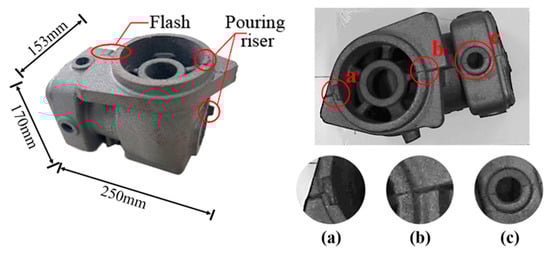
Figure 1.
Physical drawing of casting. (a) Pouring riser area. (b) Flash area. (c) Flash area.
- (2)
- Grinding system composition and working principle
The grinding execution part and the visual guiding part are the two primary components of the casting grinding visual guidance system. Figure 2 displays the whole system’s composition. The robot that performs the movement, flexible grinding device, electric spindle, emery grinding head, fixture that fixes the workpiece, and robot control cabinet make up the grinding execution. A structured light camera, camera sliding table, programming logic controller (PLC), and industrial control computer are all included in the vision guidance component. The camera data is sent via a wide area network (WAN) to the industrial personal computer (IPC), which then sends the processed grinding trajectory to the robot control cabinet, which instructs the robot to grind using the appropriate algorithm.

Figure 2.
Three-dimensional model diagram of the system.
The camera can slide longitudinally on the camera sliding table, which is situated in front of the workpiece. The camera slides to the top of the workpiece to take pictures when necessary. To prevent a collision, the camera is shifted out of the polishing area after the shot.
3. Zoned Grinding Strategy Based on Feature Point Groups
3.1. System Parameter Calibration
- (1)
- Structured light system calibration
The quality of the camera calibration has a direct impact on the correctness of the final image [11]. The imaging principle was approximated during calibration as the small-aperture imaging model depicted in Figure 3 to determine the camera’s internal characteristics. The matrix represented in Equation (1) can be used to express the relationship between the point P(x,y,z) in space and the point (u, v) projected in the pixel coordinate system after shooting, where (u0, v0) is the coordinate of the intersection of the image plane and the optical axis, s is the scaling factor used to convert pixel values into length values, R is the rotation matrix of the coordinate system, T is the offset vector of the coordinate system, etc.:
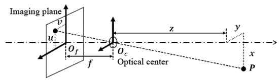
Figure 3.
Principle of keyhole imaging.
The acquired images will have a variety of distortions due to the presence of errors, so it is important to utilize the Zhang Zhengyou calibration method to correct the image aberrations [12]. To calibrate a camera using the Zhang Zhengyou method, it is necessary to collect various pixel coordinates from various positional shooting calibration plates and solve the initial values of the camera’s internal and external parameters and its aberration coefficients using a single-strain matrix and nonlinear least squares method. Finally, the maximum likelihood estimation approach is used to optimize the parameters. The transformation relationship between pixel coordinates and world coordinates can be established as illustrated in Equation (3) by substituting the compensating Equation (2) of the small-aperture model into the matrix (1), where γ is the distortion coefficient:
In structured light systems, it is also important to calibrate the projector and camera to determine the rigid transformation matrix to calculate the object’s 3D coordinate values concerning the camera. According to Figure 4, the coordinate positions of the point P in the camera coordinate systems Oc and projector coordinate systems Op are [13]:
where PP and PC are, respectively, point P’s locations in the projector and camera coordinate systems. The rotation matrices from the projector and camera coordinate systems to the global coordinate system are denoted by the letters RP and RC, respectively. The translation matrices from the projector and camera coordinate systems to the global coordinate system are denoted by the letters TP and TC, respectively. The link between PP and PC is as follows since they both represent the same point:

Figure 4.
Schematic diagram of the binocular model.
The rotation matrix R and translation vector T between the projector and camera coordinate systems shown in Equation (6) can be obtained by combining Equations (4) and (5):
- (2)
- Hand-eye calibration
To lessen the impact of dust on structured light camera photography and increase the system’s accuracy, the camera was installed using the eye outside the hand in this investigation, as illustrated in Figure 5 [14]. The idea is to install the camera outside of the hand. Following the installation of the structured light camera, the calibration plate is installed on the robot’s end flange. By capturing photos of the calibration plate in various positions, hand-eye calibration is accomplished.
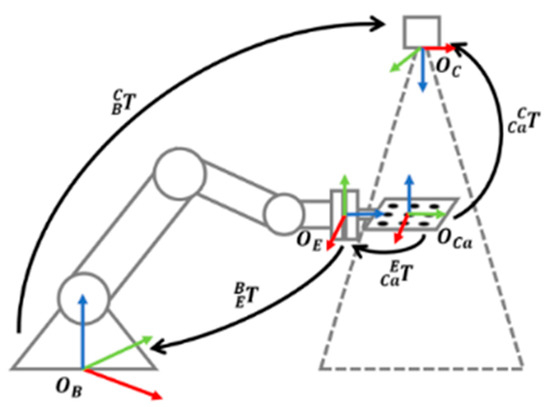
Figure 5.
The principle of hand-eye calibration.
The relationship between the coordinate systems can be obtained by transforming the calibration plate coordinate system into the camera coordinate system as Equation (7):
where is the transformation matrix of the robot base coordinate system into the camera coordinate system, is the transformation matrix of the robot end coordinate system into the base coordinate system, and is the transformation matrix of the calibration plate coordinate system into the robot end flange coordinate system.
After moving the robot and changing the position of the calibration plate, the pictures of the calibration plate are taken. The equations obtained are eliminated and the matrix vectorized to obtain Equation (8). The transformation matrix between the camera and the base coordinate system was solved by the method of least square:
The symbol “” denotes the Kronecker product, which is an operation between two matrices of arbitrary size.
3.2. Point Cloud Data Processing
- (1)
- Point cloud preprocessing
This study separates the entire point cloud into numerous voxels using voxel raster filtering in the pre-processing stage to reduce the number of point clouds and the computation of subsequent processing and to ensure the system’s operating speed. A weighted average of the voxel’s points is employed to create a single point that will replace them all [15]. The effect is shown in Figure 6a. The region of interest (ROI) is separated initially, and pass-through filtering is then used in the ROI to swiftly remove the environmental data that was acquired by the structured light camera [16]. The effect is shown in Figure 6b. To exclude outliers that do not fit the norm, statistical filtering is performed [17]. Figure 6c displays the outcome following one processing using the aforementioned technique.
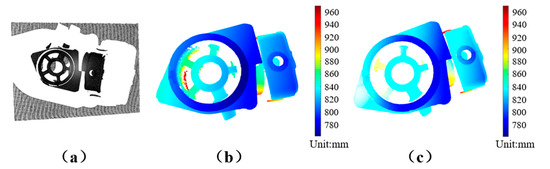
Figure 6.
Results of different point cloud pretreatment methods. (a) Rendering of voxel grid filtering. (b) Straight through filtering effect diagram. (c) Effect diagram of statistical filtering.
- (2)
- Point cloud partitioning
To eliminate part of the environmental information from the inserted castings, the random sample consensus (RANSAC) technique is utilized to calculate the error between the sample locations and the model parameters. As illustrated in Equation (9), the RANSAC algorithm chooses the best model by minimizing the cost function J [18]. Iteration can be used to find the set of interior points with the greatest number of interior points [19]. Equation (10) provides the expression for the ideal k number of model iterations [20,21]:
In Equation (9), D is the point cloud data set, L is the loss function, E is the error function corresponding to the loss function, and S is the identified model parameters. In Equation (10), p is the probability of occurrence of valid data, ω is the proportion of correct data to the overall data, and n is the minimum sample data in the point cloud. The inner point set with the highest number of inner points is the environmental information that needs to be fitted to the plane and removed.
- (3)
- Point cloud registration
By figuring out the rigid matrix transformation relationship between the two point cloud images, point cloud registration is the process of aligning two point cloud images with overlapping regions to the same coordinate system [22]. Before converting the latter coordinate system into the former through the transformation matrix, the two-point cloud maps must first be registered. Equation (11) is used to calculate how to change the coordinates of the m points under the coordinate system of the nth map to the coordinate system of the first map:
The overlapped area will result in a specific offset when the coordinates are unified. The averaging fusion algorithm converts the average value of point coordinates in a point’s field to the point’s coordinate value to guarantee the accuracy of registration. After multiple fusion calculations, the entire point cloud map of the casting can be obtained [23]. The complete point cloud map of the casting is shown in Figure 7.

Figure 7.
Complete point cloud diagram of casting.
3.3. Template Matching of Point Clouds
The computational complexity is reduced to o(nk) using the feature point feature histogram FPFH descriptor to characterize the full feature information of a region of the image. The use of the fast point feature histogram (FPFH) descriptor to describe the complete feature information of a region of the picture reduces the computational cost to o(nk) [24]. The relationship between two neighboring points Ps and Pt in space is shown in Figure 8.

Figure 8.
The relationship between two adjacent points.
The local coordinate system is established at the feature point Ps, with the normal phase vector at this point as the u-axis and the w-axis are perpendicular to the plane formed by and . The local coordinate system is established according to Equation (12):
The angle between the normal vector at point and the w-axis, the angle between and the u-axis, the angle between the normal vector at and the u-axis after projection on the uov plane. The Euclidean distance between the two points can be calculated according to Equation (13):
The aforementioned calculation was carried out for the surrounding points within the radius r of the circle’s center at point P0 (as shown in Figure 9). According to Equation (14), the final histogram is calculated using the simple point feature histogram (SPFH) of the nearby points. By contrasting the FPFH descriptors of the two-point clouds, the spatial coordinate system transformation between two-point clouds is calculated:
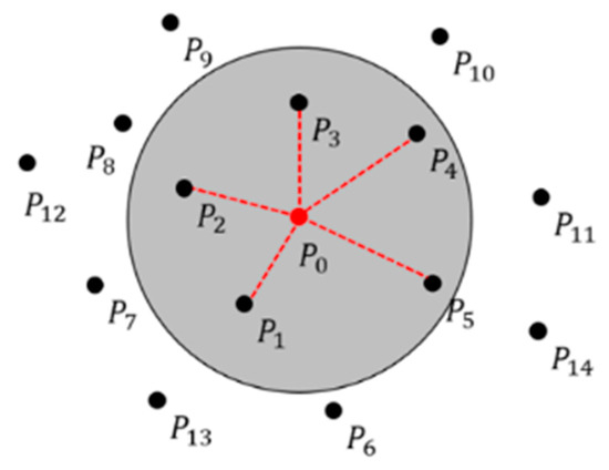
Figure 9.
FPFH calculation schematic diagram.
A local feature template is created first, and then the appropriate position in the overall point cloud is located using template matching to locate the template’s position in the target point cloud. To some extent, reducing the overall impact of the local area, the stiff transformation matrix between the two is obtained. According to the RANSAC algorithm and filtering described in Section 3.2, Figure 10 depicts the circular matching template for the top surface of the casting.

Figure 10.
Partial template.
To increase the accuracy of the template matching, the FPFH and RANSAC algorithms is used for coarse alignment, followed by the iterative closest point (ICP) technique for fine alignment. The initial value of the ICP algorithm is the transformation matrix produced from the coarse alignment, and the least-squares iterative optimization is then carried out until convergence [25,26,27]. The stiff transformation matrix for the conversion of the template to the intended point cloud is then obtained. Figure 11 depicts the results of coarse and exact alignment:
where is the point in the template point cloud, is the point transformed from to the target point cloud, is the point corresponding to on the target point cloud, n is the number of points, R is the rotation matrix, and T is the translation matrix.
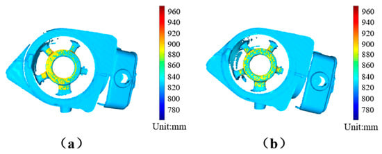
Figure 11.
Coarse and fine registration renderings. (a) Coarse alignment effect. (b) Precision matching accurate effect.
3.4. Algorithm for the Generation of the Grinding Track in the Zoned Area
Depending on the type of grinding, each region is marked out with a scribe, and the template is compared to the casting to determine its location. The difference between the two point clouds is greater than a predetermined threshold. The point cloud of the casting component that needs to be sanded and removed is obtained by statistical filtering to remove the outlier points, and the amount of sanding in each area is then determined by deduction from the generated standard template. The point clouds of some areas after extraction of the grinding volume are shown in Figure 12a–d.

Figure 12.
Grinding amount extraction point cloud map. (a) Ring flash point cloud. (b) Pouring riser point cloud. (c) Small circle flash point cloud. (d) Plane flash point cloud.
The equation ax + by + cz + d = 0 for the plane in which the component to be ground is located is found using the RANSAC method for a circular PLF. For ellipse fitting, the circular PLF is projected onto the plane. After several iterations, the elliptical fitting result is reached, as illustrated in Figure 13, where the ellipse equation is .

Figure 13.
Ellipse fitting result graph.
Since chamfering grinding is employed, Equations (17) and (18) must be adopted to adjust the trajectory and posture of the grinding head. When discrete points are present, their unit normal vector and unit tangent vector :
The relationship between the grinding trajectory and the fitted ellipse is shown in Figure 14 and the relationship between the two is shown in Equations (19)–(21). According to Equations (19)–(21), we can find the points on the grinding track:
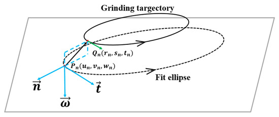
Figure 14.
The relationship between grinding track and fitting ellipse.
It is necessary to grind the CFH in several layers. The same technique used to create the circular PLF trajectory is used to create the point cloud image. The grinding can be finished in one cut if the maximum distance D between the points in the point cloud and the line is smaller than a predetermined threshold. Multiple grinding is necessary if it exceeds the threshold value, and the maximum distance D is updated following each grinding. The number of grinding sessions should be recalculated. The moving trajectory and posture of the tool coordinate system are produced by coordinate transformation after the grinding trajectory or the spots on the grinding trajectory are determined by the calculation above. Figure 15a depicts the PLF grinding tool’s position, and Figure 15b depicts the CFH’s path.

Figure 15.
Grinding head position trajectory. (a) Pose trajectory diagram of the flash grinding tool. (b) Pouring riser grinding pose trajectory diagram.
4. Simulation Experimental Verification
4.1. Simulation Experimental Principle
The corresponding program is used to simulate this study. Before taking a point cloud image, a blank casting that serves as a template casting is hand ground to within tolerance. The extra point cloud is then deleted after shooting the empty point cloud image, generating the grinding trajectory using the method mentioned above, and grinding and simulating the point cloud image. The ground point cloud image and the template casting are compared horizontally. Finally, several point clouds of blank casting are captured on camera and ground numerous times. A vertical comparison compares two photographs of ground casting point clouds and records the results.
4.2. Analysis of Simulation Result
Figure 16 depicts the relationship between the distance and the number of points, and Table 1 displays the longitudinal comparison data between template casting and ground casting. There are 22,443 points in total within the PLF ROI, and 243 of those points (or 1.08 percent) are bigger than the free tolerance (0.5 mm) from the template. There are 5418 points in the CFH ROI, and 8 of them, or 0.15 percent, are further away from the template than the free tolerance (0.5 mm). The vast majority of the longitudinal range’s points comply with the tolerance and grinding standards.

Figure 16.
Vertical comparison picture.

Table 1.
Vertical comparison data table of castings.
Table 2 displays the lateral comparison information between the template casting and the ground casting, and Figure 17 depicts the relationship between the distance and the number of points. There are 16,889 points in the PLF ROI, and 98 of them, or 0.58 percent, are further apart than the free tolerance (0.5 mm). In total, 4817 points make up the CFH ROI, and 7 of those (or 0.14 percent) fall beyond the free tolerance (0.5 mm), indicating a more satisfactory grinding result. The overwhelming majority of transverse range points fall inside the tolerance range as well, demonstrating that the grinding system developed for this study complies with the specifications. This further demonstrates the good consistency of the ground finished castings.
Table 2.
Horizontal comparison data table of castings.

Figure 17.
Horizontal comparison picture.
The bigger part of the gap is mostly caused by the individual variances between the castings while the lesser part of the distance is caused by camera mistakes and positioning errors. According to the statistics for both the horizontal and vertical point clouds, the vertical point cloud has a higher percentage of points with distances greater than the free tolerance, and the effect is also slightly worse than the horizontal. Both, however, can perform the grinding duty and are within the tolerance of 0.5 mm. The system in this study can adapt to the distinctive properties of castings and provide efficient grinding trajectories for custom grinding castings, according to the simulation results.
5. Conclusions
- (1)
- This study suggests the use of pump body casting blanks as the grinding object in a feature point-based grinding technique for zoning castings. It can produce grinding trajectories to address the issue of poor consistency between castings and extract the individual changes between castings. Comparison of the system to the template castings allowed us to confirm its efficacy.
- (2)
- The local point clouds are described using the FPFH descriptor, and the pictures are coarse aligned using the RANSAC algorithm. Based on the coarse alignment, the ICP technique is used to stitch the point clouds taken at various angles and places. This method yields an accurate overall casting point cloud.
- (3)
- The area is split according to the casting characteristics, and the extraction of the grinding volume is carried out for each section. According to the various grinding types, the algorithm creates the actual grinding trajectory and posture in the point cloud, and the grinding effect is generally acceptable.
In the future, we will integrate robot haptics apps into the hand robot control system to deliver real-time feedback on the grinding condition. This system may modify the grinding trajectory in real-time in response to feedback to increase the quality of the grinding by correlating the grinding volume to the grinding force. Additionally, we will use machine learning to eliminate the need for sanding beforehand and free up manpower.
Author Contributions
Conceptualization, M.Z. and T.S.; methodology, M.Z. and Z.J.; software, M.Z. and Z.J.; validation, Z.J. and W.D.; formal analysis, M.Z. and T.S.; writing—original draft preparation, M.Z.; writing—review and editing, C.L. and Y.C.; funding acquisition, T.S. and Y.C. All authors have read and agreed to the published version of the manuscript.
Funding
This research was funded by Project for the Jiaxing City Science and Technology Plan, grant number 2021AD10019; Key Research and Development Program of Jilin Province, grant number 20210203175SF; Foundation of Education Bureau of Jilin Province under grant, No: JJKH20220988KJ; Aeronautical Science Foundation of China under grant, No: 2019ZA0R4001; National Natural Science Foundation of China under grant, No: 51505174; Interdisciplinary Integration Innovation and Cultivation Project of Jilin University under grant, No: JLUXKJC2020105.
Institutional Review Board Statement
Not applicable.
Informed Consent Statement
Informed consent was obtained from all subjects involved in the study.
Data Availability Statement
Data sharing not applicable.
Acknowledgments
The authors are grateful to the editor and anonymous reviewers for their constructive comments and suggestions which have improved this paper.
Conflicts of Interest
The authors declare no conflict of interest.
References
- Zeng, X.; Yang, X. Effect of Temperature on Machining Size of Aluminum Alloy. In Proceedings of the 2021 Chongqing Foundry Annual Meeting, Chongqing, China, 12–14 May 2021; pp. 306–307. [Google Scholar]
- Lv, Z.; Zhang, Y.L. Finite Element Analysis of High Temperature Ti-1100 Titanium Alloy Deformation During Casting Process. Foundry Technol. 2017, 38, 2459–2461. [Google Scholar] [CrossRef]
- Su, Y.P.; Chen, X.Q.; Zhou, T.; Pretty, C.; Chase, G. Mixed Reality-Enhanced Intuitive Teleoperation with Hybrid Virtual Fixtures for Intelligent Robotic Welding. Appl. Sci. 2021, 11, 11280. [Google Scholar] [CrossRef]
- Kosler, H.; Pavlovčič, U.; Jezeršek, M.; Možina, J. Adaptive Robotic Deburring of Die-cast Parts with Position and Orientation Measurements Using A 3D Laser-triangulation Sensor. Stroj. Vestn.-J. Mech. Eng. 2016, 62, 207–212. [Google Scholar] [CrossRef]
- Ji, P.F.; Hou, F.B.; Lu, C. Design of Casting Grinding Robot Based on Vision Technology. Mach. Tool HYD Raulics 2021, 49, 30–33. [Google Scholar]
- Wang, G.L.; Wang, Y.Q.; Zhang, L.; Zhao, J.; Zhou, H.B. Development and Polishing Process of A Mobile Robot Finishing Large Mold Surface. Mach. Sci. Technol. 2014, 18, 603–625. [Google Scholar] [CrossRef]
- Bedaka, A.K.; Vidal, J.; Lin, C.Y. Automatic Robot Path Integration Using Three-dimensional Vision and Offline Programming. Int. J. Adv. Manuf. Technol. 2019, 102, 1935–1950. [Google Scholar] [CrossRef]
- Wan, G.Y.; Wang, G.F.; Li, F.D.; Zhu, W.J. Robotic Grinding Station Based on Visual Positioning and Trajectory Planning. Comput. Integr. Manuf. Syst. 2021, 27, 118–127. [Google Scholar] [CrossRef]
- Wang, D.; Peters, F.E.; Frank, M.C. A Semiautomatic, Cleaning Room Grinding Method for the Metalcasting Industry. J. Manuf. Sci. Eng. 2017, 139, 121017. [Google Scholar] [CrossRef]
- Zhu, X.H.; Mo, X.D.; Wang, X.F.; Wang, C.F. Application Research of Industrial Robot in Aluminum Casting Deburring. Modul. Mach. Tool Autom. Manuf. Tech. 2014, 124–126+130. [Google Scholar] [CrossRef]
- Liu, Y.; Li, T.F. Reaserch of The Improvement of Zhang’s Camera Calibration Method. Opt. Tech. 2014, 40, 565–570. [Google Scholar] [CrossRef]
- Zhang, Z.Y. A Flexible New Technique for Camera Calibration. IEEE Trans. Pattern Anal. Mach. Intell. 2000, 22, 1330–1334. [Google Scholar] [CrossRef] [Green Version]
- Liu, F.C.; Xie, M.H.; Wang, W. Stereo Calibration Method of Binocular Vision. Comput. Eng. Des. 2011, 32, 1508–1512. [Google Scholar] [CrossRef]
- Ge, S.Q.; Yang, Y.H.; Zhou, Z.W. Research and Application of Robot Hand-eye Calibration Method Based on 3D Depth Camera. Mod. Electron. Tech. 2022, 45, 172–176. [Google Scholar] [CrossRef]
- Li, H.; Fan, Y.Q.; Liu, H.J. Point cloud map processing method based on voxel raster filter. Pract. Electron. 2021, 45–48. [Google Scholar] [CrossRef]
- Huang, H. Research on Position and Pose Recognition Technology of Randomly Stacked Bars Based on Point Clouds. Ph.D. Thesis, Harbin Institute of Technology, Harbin, China, 2021. [Google Scholar]
- Li, R.B. Research on Point Cloud Data Reduction Method Based on Integrated Filtering Optimization and Feature Participation. Ph.D. Thesis, Kunming University of Science and Technology, Kunming, China, 2021. [Google Scholar]
- Yan, L.J.; Huang, Y.M.; Zhang, Y.H.; Tang, T.; Xia, Y.X. Research on The Application of RANSAC Algorithm In Electro-optical Tracking of Space Targets. Opto-Electron. Eng. 2019, 46, 40–46. [Google Scholar] [CrossRef]
- Peng, X.S.; Lu, A.J.; Huang, J.W.; Chen, B.Y.; Ding, J. Mesh RANSAC Segmentetion and Counting of 3D Laser Point Cloud. Appl. Laser 2022, 42, 54–63. [Google Scholar] [CrossRef]
- Xu, G.G.; Pang, Y.J.; Bai, Z.X.; Wang, Y.L.; Lu, Z.W. A fast point clouds registration algorithm for laser scanners. Appl. Sci. 2021, 11, 3426. [Google Scholar] [CrossRef]
- Liu, Y.K.; Li, Y.Q.; Liu, H.Y.; Sun, D.; Zhao, S.B. An Improved RANSAC Algorithm for Point Cloud Segmentation of Complex Building Roofs. J. Geo-Inf. Sci. 2021, 23, 1497–1507. [Google Scholar] [CrossRef]
- Li, J.J.; An, Y.; Qin, P.; Gu, H. 3D Color Point Cloud Registration Based on Deep Learning Image Descriptor. J. Dalian Univ. Technol. 2021, 61, 316–323. [Google Scholar] [CrossRef]
- Kang, X.; Li, S.; Benediktsson, J.A. Feature Extraction of Hyperspectral Images with Image Fusion and Recursive Filtering. IEEE Trans. Geosci. Remote Sens. 2014, 52, 3742–3752. [Google Scholar] [CrossRef]
- Rusu, R.B.; Blodow, N.; Beetz, M. Fast Point Feature Histograms (FPFH) for 3D registration. In Proceedings of the IEEE International Conference on Robotics & Automation, Kobe, Japan, 12–17 May 2009. [Google Scholar]
- Liu, Y.Z.; Zhang, Q.; Lin, S. Improved ICP Point Cloud Registration Algorithm Based on Fast Point Feature Histogram. Laser Optoelectron. Prog. 2021, 58, 283–290. [Google Scholar] [CrossRef]
- Qiao, J.W.; Wang, J.J.; Xu, W.S.; Lu, Y.P.; Hu, Y.W.; Wang, Z.Y. Laser point cloud stitching based on iterative closest point algorithms. J. Shandong Univ. Technol. (Nat. Sci. Ed. ) 2020, 34, 46–50. [Google Scholar] [CrossRef]
- Wang, Z.J.; Jia, K.B.; Chen, J.P. High Precision Reconstruction Method of Vehicle Chassis Contour Based on ICP Algorithm. In Proceedings of the 15th National Conference on Signal and Intelligent Information Processing and Application, Chongqing, China, 19 August 2022; pp. 106–111+190. [Google Scholar]
Publisher’s Note: MDPI stays neutral with regard to jurisdictional claims in published maps and institutional affiliations. |
© 2022 by the authors. Licensee MDPI, Basel, Switzerland. This article is an open access article distributed under the terms and conditions of the Creative Commons Attribution (CC BY) license (https://creativecommons.org/licenses/by/4.0/).