Evaluating the Effectiveness of Text Pre-Processing in Sentiment Analysis

Abstract

Practical demands and academic challenges have both contributed to making sentiment analysis a thriving area of research. Given that a great deal of sentiment analysis work is performed on social media communications, where text frequently ignores the rules of grammar and spelling, pre-processing techniques are required to clean the data. Pre-processing is also required to normalise the text before undertaking the analysis, as social media is inundated with abbreviations, emoticons, emojis, truncated sentences, and slang. While pre-processing has been widely discussed in the literature, and it is considered indispensable, recommendations for best practice have not been conclusive. Thus, we have reviewed the available research on the subject and evaluated various combinations of pre-processing components quantitatively. We have focused on the case of Twitter sentiment analysis, as Twitter has proved to be an important source of publicly accessible data. We have also assessed the effectiveness of different combinations of pre-processing components for the overall accuracy of a couple of off-the-shelf tools and one algorithm implemented by us. Our results confirm that the order of the pre-processing components matters and significantly improves the performance of naïve Bayes classifiers. We also confirm that lemmatisation is useful for enhancing the performance of an index, but it does not notably improve the quality of sentiment analysis.

1. Introduction

Sentiment analysisencompasses a series of methods and heuristics for detecting and extracting subjective information, such as opinions, emotions, and attitudes from language [1]. Although it originated in the text subjectivity analysis performed by computational linguists in the 1990s [2,3], which was later enhanced by studies about public opinion at the beginning of the 20th century, the proliferation of publications on sentiment analysis did not start until the Web became widespread [4]. The Web and social media in particular have created a large corpora for academic and industrial research on sentiment analysis [5]. Examples of this can be found in the various applications of sentiment analysis investigated thus far: product pricing [6], competitive intelligence [7], market analysis [8], election prediction [9], public health research [10], syndromic surveillance [11], and many others. The vast majority of papers on sentiment analysis has been written after 2004 [12], making it one of the fastest growing research areas.

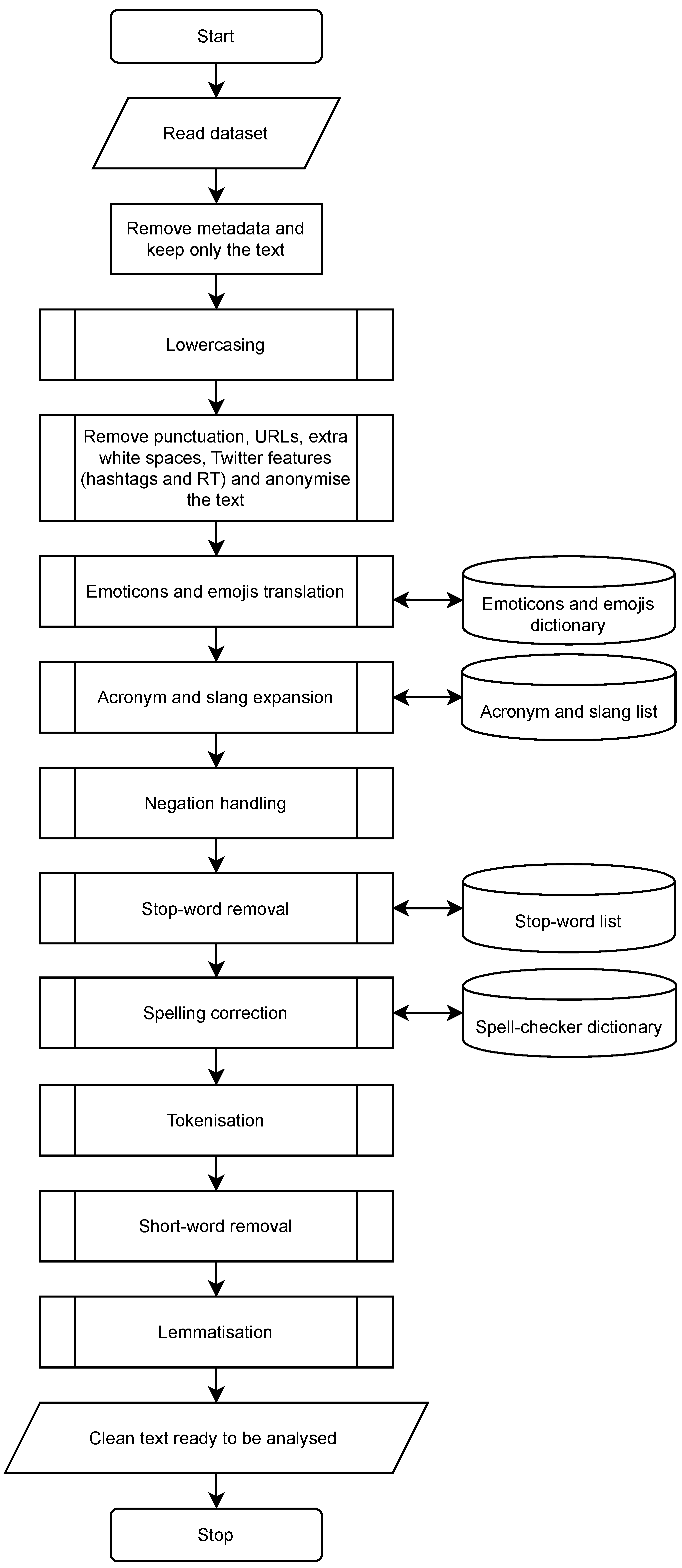
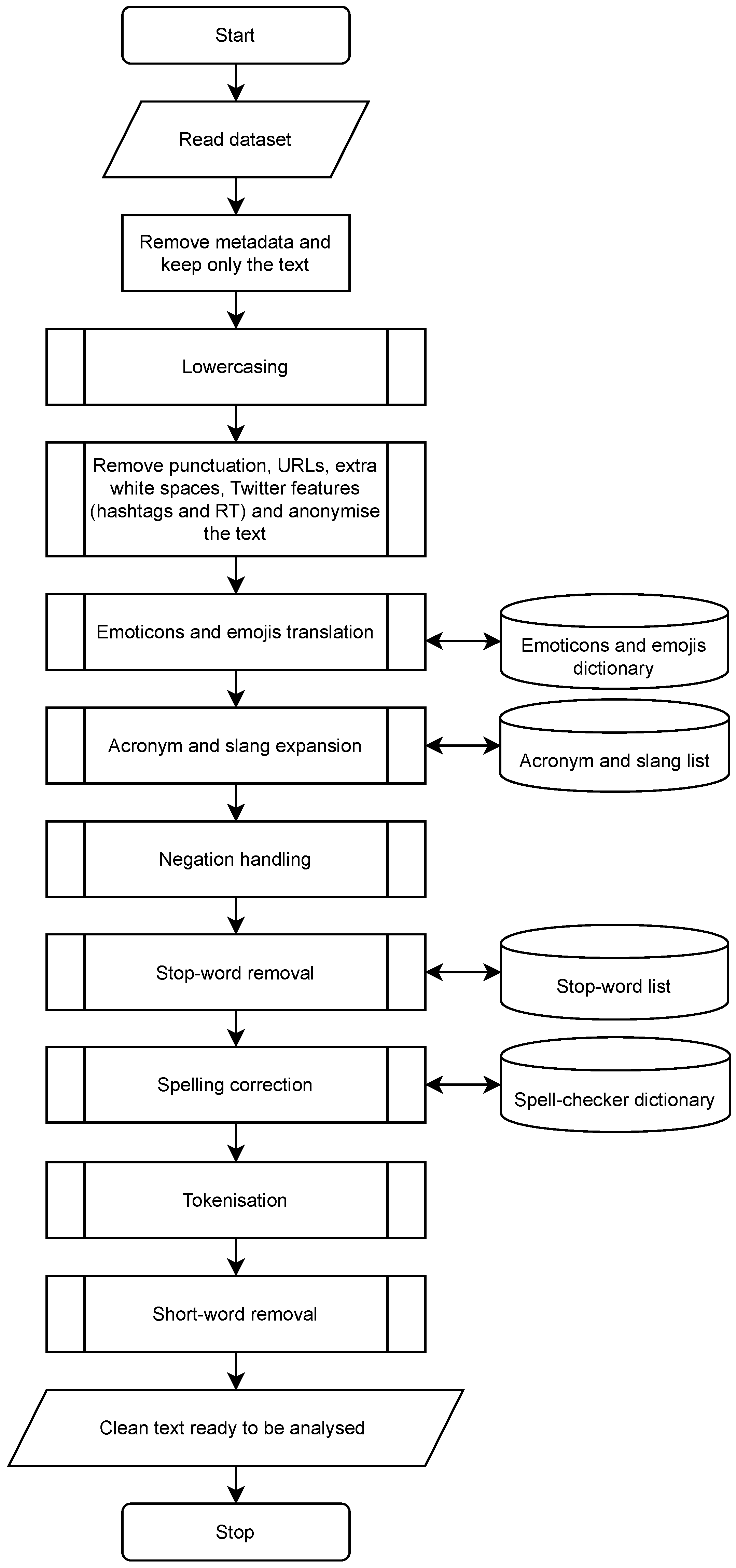
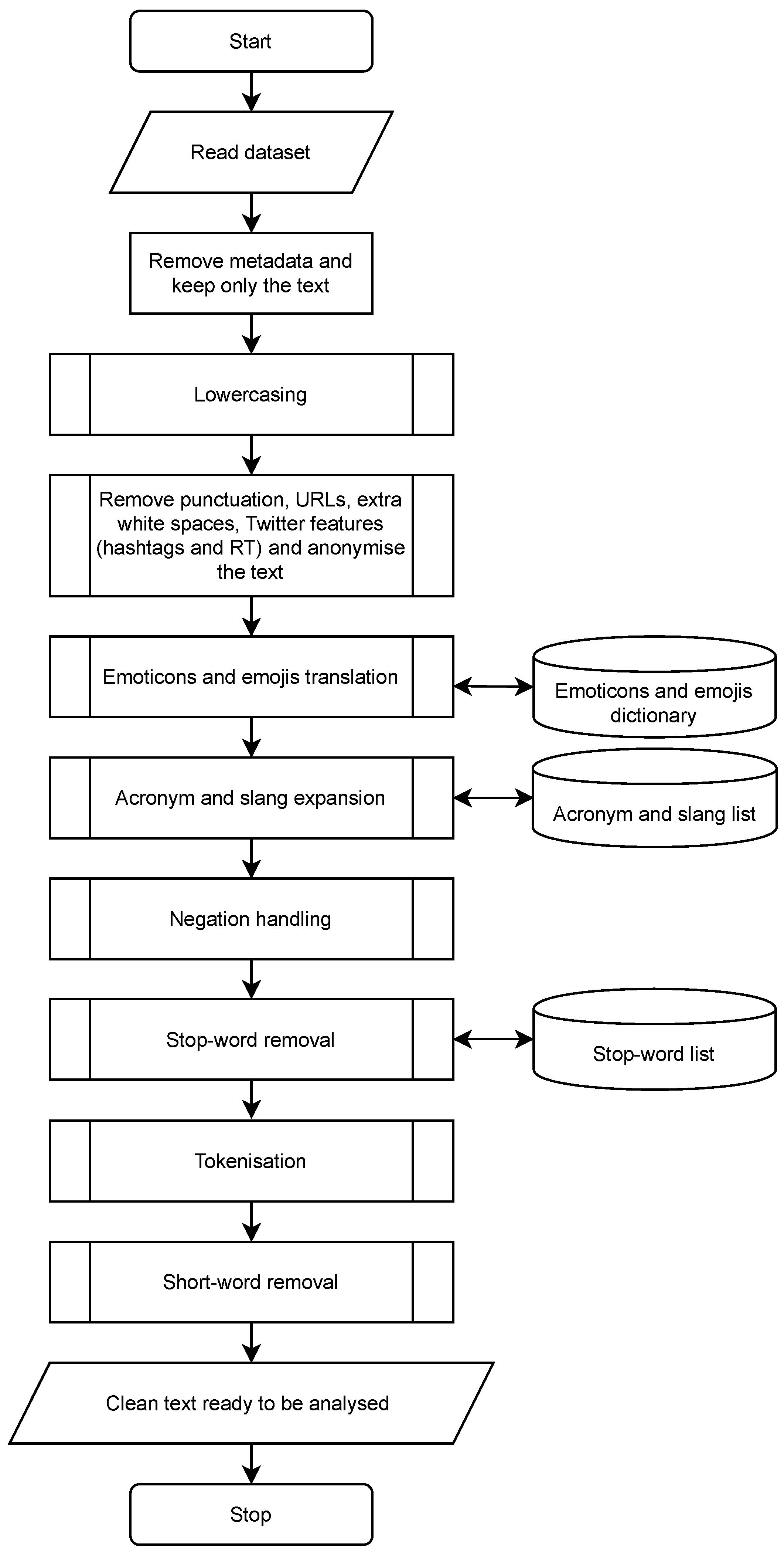
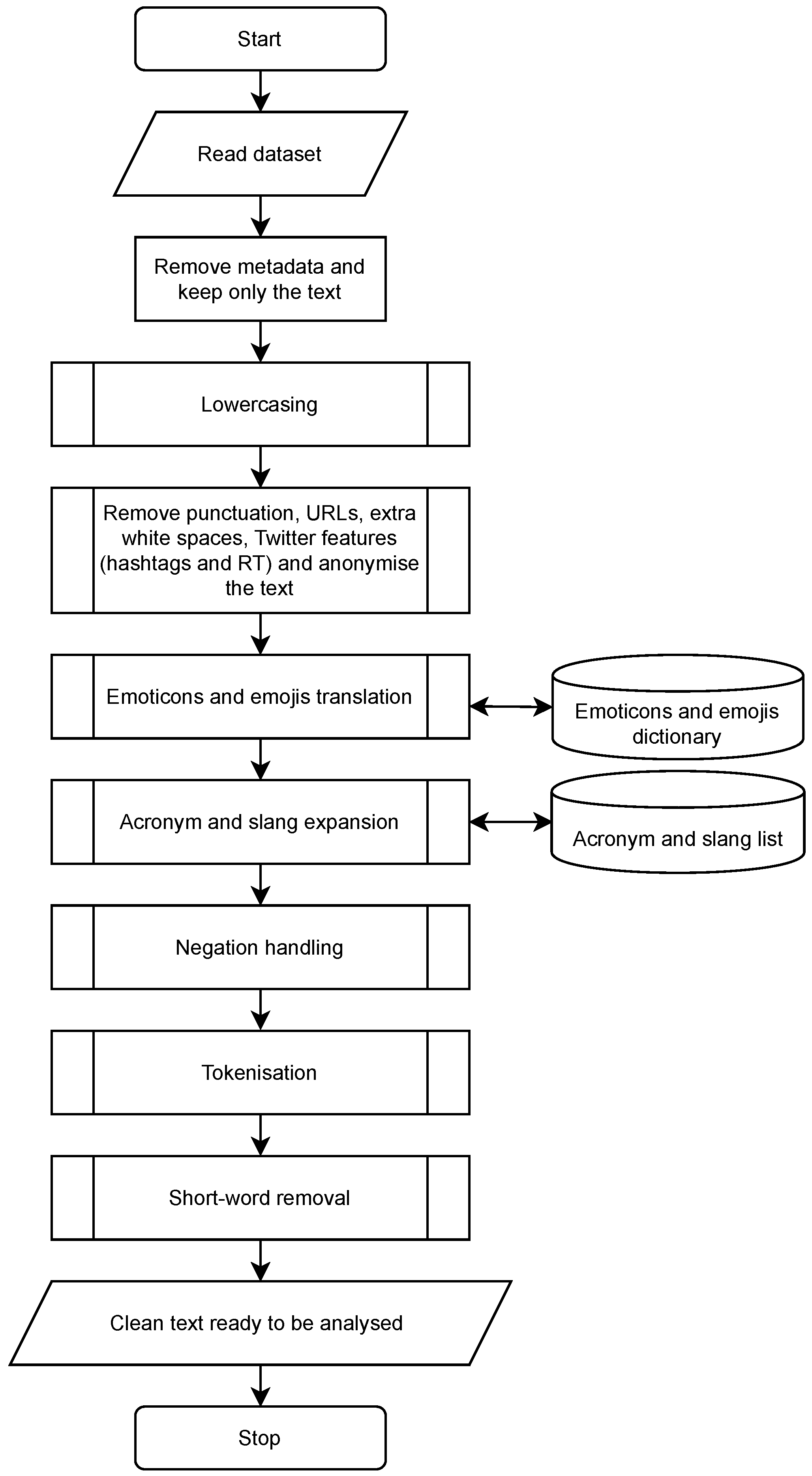
Sentiment analysis requires pre-processing components to structure the text and extract features that can later be exploited by machine learning algorithms and text mining heuristics. Generally, the purpose of pre-processing is to separate a set of characters from a text stream into classes, with transitions from one state to the next on the occurrence of particular characters. By careful consideration of the set of characters—punctuation, white spaces, emoticons, and emojis—arbitrary text sequences can be handled efficiently.

Tokenising a stream of characters into a sequence of word-like elements is one of the most critical components of text pre-processing [13]. For the English language, it appears trivial to split words by spaces and punctuation, but some additional knowledge should be taken into consideration, such as opinion phrases, named entities, and stop-words [14]. Previous research suggests that morphological transformations of language—that is, an analysis of what we can infer about language based on structural features [15]—can also improve our understanding of subjective text. Examples of these are stemming [16] and lemmatisation [17]. Lately, researchers working on word-embeddings and deep-learning based approaches have recommended that we should use techniques such as word segmentation, part-of-speech tagging, and parsing [18].

All the decisions made about text pre-processing have proved crucial to capturing the content, meaning, and style of language. Therefore, pre-processing has a direct impact on the validity of the information derived from sentiment analysis. However, recommendations for the best pre-processing practice have not been conclusive. Thus, we aim to evaluate various combinations of pre-processing components quantitatively. To this extent, we have acquired a large collection of Twitter [19] data through Kaggle [20], the online data science platform and tested a number of pre-processing flows—sequences of components that implement methods to clean and normalise text. We also assessed the impact of each flow in the accuracy of a couple of off-the-shelf sentiment analysis tools and one supervised algorithm implemented by us.

It is important to clarify that we are not intending to develop a new sentiment analysis algorithm. Instead, we are interested in identifying pre-processing components that can help existing algorithms to improve their accuracy. Thus, we have tested our various pre-processing components with two off-the-shelf classifiers and a basic naïve Bayes classifier [21]. As their name indicates, the off-the-shelf classifiers are generic and not tailored to specific domains. However, those classifiers were chosen specifically because they are used widely and therefore our conclusions may be relevant to a potentially larger audience. Lastly, we chose the naïve Bayes classifier as a third option, because it can easily be reproduced to achieve the same benefits that will be discussed later. Our results confirm that the order of the pre-processing components makes a difference. We have also encountered that the use of lemmatisation, while useful for reducing inflectional forms of a word to a common base, does not improve sentiment analysis significantly.

The reminder of this paper is organised as follows. Section 2 reviews the related work. Section 3 describes the corpus used for our experiments, and the text pre-processing components and flows tested. Section 4 presents our results, and, finally, Section 5 offers our conclusions.

2. Related Work

As the number of papers on sentiment analysis continues to increase—largely as a result of social media becoming an integral part of our everyday lives—the number of publications on text pre-processing has increased too. According to Mäntylä et al. [12], nearly 7000 papers on sentiment analysis have been indexed by the Scopus database [22] thus far. However, 99% of those papers were indexed after 2004 [12].

Over the past two decades, YouTube [23] and Facebook [24] have grown considerably. Indeed, YouTube and Facebook have reached a larger audience than any other social platform since 2019 [25]. Facebook, in particular, has held a steady dominance over the social media market throughout recent years. In the UK, for example, which is where we carried out our study, Facebook has a market share of approximately 52.40%, making it the most popular platform as of January 2021. Twitter, on the other hand, has achieved a market share of 25.45%, emerging as the second leading platform as of January 2021 [26].

Although Twitter’s market share falls behind Facebook’s, the amount of Twitter’s publicly available data is far greater than that corresponding to Facebook. This makes Twitter remarkably attractive within the research community, and that is why we have undertaken all our work using it.

Table 1. Four relevant papers on text pre-processing indexed by Scopus.

Paper	Scopus Citations
Sun et al. A Review of Natural Language Processing
Techniques for Opinion Mining Systems. Information Fusion	225
2017, 36, 10–25 [29].
Jianqiang et al. Comparison Research on Text
Pre-processing Methods on Twitter Sentiment Analysis.	140
IEEE Access 2017, 5, 2870–2879 [30].
Petz et al. Reprint of: Computational Approaches for
Mining Users Opinions on the Web 2.0. Information	57
Processing & Management2015, 51, 510–519 [31].
Angiani et al. A Comparison between Preprocessing
Techniques for Sentiment Analysis in Twitter. Proceedings	35
of the International Workshop on Knowledge Discovery
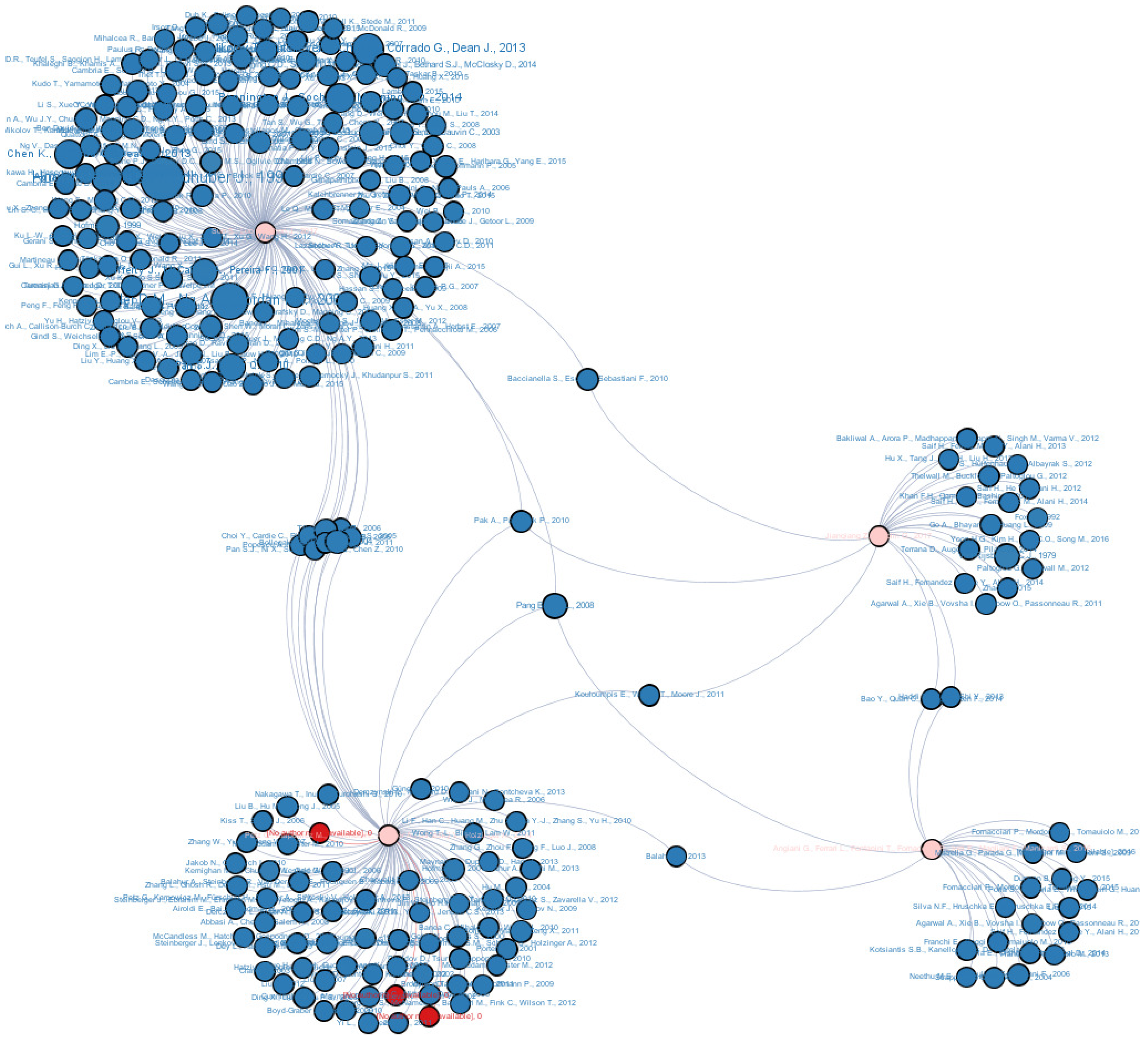
on the WEB, 2016 [32].

 lists four of the most cited papers on text pre-processing available on Scopus. Such papers along with their references account for 279 publications, which are all represented in Figure A1 in Appendix A. Pink circles in Figure A1 represent the four papers displayed in Table 1, red circles represent the earliest publications on the subject—these are publications mostly related to the Lucene Search Engine [27]—and blue circles represent the rest of the papers. The size of the circles depends on the number of citations of the corresponding paper: the larger the circle is, the more citations the paper has. The links between the papers denote the citation relationship—paper A is linked to paper B if A cites B. Figure A1 was produced with Gephi [28], an open-source network analysis and visualisation software package.

The size and connectivity of the network displayed in Figure A1 in Appendix A, which is based on only four papers, shows that the body of literature on text pre-processing is large and keeps growing. However, it is still unclear which pre-processing tools should be employed, and in which order. Thus, we have evaluated various pre-processing flows quantitatively and we will present our conclusions here.

A couple of influential publications that have followed a similar approach to what we aim to achieve are Angiani et al. [32] and Jianqiang et al. [30]. These publications are included in Table 1 and have stated the sequences of pre-processing components that they have examined and the order in which they have examined them. Table 2 displays these sequences as pre-processing flows. The first row of Table 2 indicates the datasets used by the corresponding authors to test their approaches. The remaining rows in Table 2 display the actual steps included in the pre-processing flows. As explained before, researchers have recommended the use of text pre-processing techniques before performing sentiment analysis—an example of this can be found in Fornacciari et al. [33]. However, we are not only interested in using pre-processing techniques but also in comparing different pre-processing flows and identifying the best.

Pre-processing is often seen as a fundamental part of sentiment analysis [32], but it rarely is evaluated in detail. Consequently, we wanted to assess the effect of pre-processing on some off-the-shelf sentiment analysis classifiers that have become popular—namely VADER [34] and TextBlob [35]. To compare and contrast these off-the-shelf classifiers with other alternatives, we have implemented our own classifier, based on the naïve Bayes algorithm [21]. Additionally, we took advantage of this opportunity to examine some components which have not been researched broadly in the literature. For instance, most of the existing literature on English sentiment analysis refers to stemming as a pre-processing step—see, for instance, Angiani et al. [32]. However, we have also evaluated lemmatisation [36], which is a pre-processing alternative that has been frequently overlooked.

Despite all the recent NLP developments, determining the sentiment expressed in a piece of text remains a problem that has not been fully solved. Issues such as sarcasm or negation remain largely unsolved [37]. Our main contribution lies precisely in identifying pre-processing components that can pave the way to improving the state of the art.

Table 2. Two text pre-processing flows evaluated in the relevant literature.

Angiani et al.’s flow [32]: Tested	Jianqiang et al.’s flow [30]: Tested
on two SemEval Twitter datasets	on five manually annotated Twitter
from 2015 [38] and 2016 [39].	datasets (reported in [30]).
In order to keep only significant	Replace negative mentions—that
information, remove URLs, hashtags	is, replace won’t, can’t, and n’t
(for example, #happy) and user	with will not, cannot, and not,
mentions (for example, @BarackObama).	respectively.
Replace tabs and line breaks	Remove URLs. Most researchers
with a blank, and quotation	consider that URLs do not carry
marks with apostrophes.	any valuable information regarding
	the sentiment of a tweet.
Remove punctuation, except for	Revert words that contain
apostrophes (because apostrophes	repeated characters to their
are part of grammar constructs,	original English forms. For
such as the genitive).	example, revert cooooool to cool.
Remove vowels repeated in sequence	Remove numbers. In general,
at least three times to normalise	numbers are of no use when
words. For example, the words cooooool	measuring sentiment.
and cool will become the same.
Replace sequences of a and h with a	Remove stop words. Multiple
laugh tag—laughs are typically	lists are available, but the classic
represented as sequences of the	Van Rijsbergen stop list [40] was
characters a and h.	selected by Jianqiang et al. [30].
Convert emoticons into corresponding	Expand acronyms to the original
tags. For example, convert :) into	words by using an acronym
smile_happy. The list of emoticons	dictionary, such as the Internet &
is taken from Wikipedia [41].	Text Slang Dictionary & Translator [42].
Convert the text to lower case, and
remove extra blank spaces.
Replace all negative constructs (can’t,
isn’t, never, etc.) with not.
Use PyEnchant [43] for the detection
and correction of misspellings.
Replace insults with the tag bad_word.
Use the Iterated Lovins Stemmer
[44] to reduce nouns, verbs, and adverbs
which share the same radix.
Remove stop words.

Table 2. Two text pre-processing flows evaluated in the relevant literature.

Angiani et al.’s flow [32]: Tested	Jianqiang et al.’s flow [30]: Tested
on two SemEval Twitter datasets	on five manually annotated Twitter
from 2015 [38] and 2016 [39].	datasets (reported in [30]).
In order to keep only significant	Replace negative mentions—that
information, remove URLs, hashtags	is, replace won’t, can’t, and n’t
(for example, #happy) and user	with will not, cannot, and not,
mentions (for example, @BarackObama).	respectively.
Replace tabs and line breaks	Remove URLs. Most researchers
with a blank, and quotation	consider that URLs do not carry
marks with apostrophes.	any valuable information regarding
	the sentiment of a tweet.
Remove punctuation, except for	Revert words that contain
apostrophes (because apostrophes	repeated characters to their
are part of grammar constructs,	original English forms. For
such as the genitive).	example, revert cooooool to cool.
Remove vowels repeated in sequence	Remove numbers. In general,
at least three times to normalise	numbers are of no use when
words. For example, the words cooooool	measuring sentiment.
and cool will become the same.
Replace sequences of a and h with a	Remove stop words. Multiple
laugh tag—laughs are typically	lists are available, but the classic
represented as sequences of the	Van Rijsbergen stop list [40] was
characters a and h.	selected by Jianqiang et al. [30].
Convert emoticons into corresponding	Expand acronyms to the original
tags. For example, convert :) into	words by using an acronym
smile_happy. The list of emoticons	dictionary, such as the Internet &
is taken from Wikipedia [41].	Text Slang Dictionary & Translator [42].
Convert the text to lower case, and
remove extra blank spaces.
Replace all negative constructs (can’t,
isn’t, never, etc.) with not.
Use PyEnchant [43] for the detection
and correction of misspellings.
Replace insults with the tag bad_word.
Use the Iterated Lovins Stemmer
[44] to reduce nouns, verbs, and adverbs
which share the same radix.
Remove stop words.

3. Materials and Methods

3.1. Experimental Dataset

Our research was conducted using a dataset retrieved from Twitter. As stated above, such dataset has been made publicly available by Kaggle [20], a platform that hosts data science competitions for business problems, recruitment, and academic research. Our dataset was originally taken from the Crowdflower’s Data for Everyone Library, now known as the Datasets Resource Center [45]. It contains 13,871 tweets published in relation to the first Grand Old Party (GOP) debate held among the candidates of the Republican Party who were looking for nomination in the 2016 US Presidential election. There were 12 debates in total, but the one that corresponds to our experimental dataset is the first one.

The debate commented on by the tweets in our dataset took place in Cleveland, Ohio, on 6 August 2015, starting at 17:00 EDT and finishing at 21:00 EDT. However, the tweets were collected over a 17 h period, approximately, starting at 17:44:53 EDT and finishing the following day, 7 August 2015, at 10:12:32 EDT [45]. Figure 1 shows the number of tweets captured per hour. As it can be seen, the largest number of tweets was published between 01:00 and 08:00, with two clear peaks at around 02:00 and 06:00. While the corpus does not seem to be evenly balanced across the time of collection, we took it exactly as it was published by Kaggle. The debate was seen on television by 24 million viewers, making it the most watched live broadcast for a non-sporting event in cable television history [46].

A group of contributors created the necessary metadata to annotate the tweets with information, such as how relevant the tweets were to the GOP debate, which candidates were mentioned in each tweet, what subjects were discussed, and what sentiment polarity value—positive, negative, or neutral—could be associated with each tweet [47]. A total of 61% of the tweets were classified as negative, 23% as positive, and 16% as neutral. Each tweet was associated with a confidence sentiment value, which is an indicator of the degree of reliance the contributors have regarding the overall sentiment expressed in the tweet. A total of 5370 tweets had a confidence sentiment value between 0.96 and 1; 6779 tweets between 0.59 and 0.72; and 1621 between 0.31 and 0.39. Figure 2 shows the proportion of positive, negative, and neutral tweets in the dataset which had a high confidence sentiment value—between 0.96 and 1.

Predictably, the hashtag #GOPDebate, which is the hashtag employed to refer generically to the twelve presidential debates and nine forums that were held between the candidates for the Republican Party’s nomination for the presidency in the 2016 US election, was the most frequent term in the dataset. The names and last names of the candidates—Donald Trump, Jeb Bush, Scott Walker, Mike Huckabee, Ben Carson, Ted Cruz, Marco Rubio, Rand Paul, Chris Christie, and John Kasich—were also among the most frequent terms. The television network—Fox News Channel—is constantly referred to in the dataset as well. Figure 3 displays a word cloud created with the terms found in the experimental dataset. Given that frequency is not the best indicator of relevance [48], we chose TF-IDF [15] to rank the terms. The higher the TF-IDF score is, the larger the font size used to display it on the cloud is. The cloud was produced using the Python WordCloud library [49].

3.2. Pre-Processing Components

To assess the impact of pre-processing on the accuracy of Twitter sentiment classifiers, we implemented the next 12 pre-processing components. We will describe them first, and we will later discuss the order in which we execute them.

• Lowercasing: We convert to lowercase all the characters in the dataset, as opposed to capitalising proper names, initials, and words at the start of the sentence. Capitalisation is complex in Twitter, because users tend to avoid capital letters, as this lends a tone of informality to the conversation that makes the messages more speech-like [50]. Therefore, lowercasing everything seems to be the most practical approach.
• Removal of URLs and Twitter features: We remove URLs entirely, because we cannot estimate the sentiment of an online resource—web page, picture, or anything else associated with a URL. We also remove the hashtag character, but not the keywords or phrases comprised within the hashtags—for example, we remove the # character from #happy, but not the word happy, because it can have a sentiment-related connotation. We also remove the characters RT at the beginning of the tweets. RT is used to indicate the re-tweeting—or re-posting—of someone else’s tweets.
• Removal of unnecessary spaces: Identifying spaces between characters is critical, as spaces are considered word boundaries. Regrettably, splitting a character sequence where spaces occur can also split what should be regarded as a single “token”. This happens commonly with names—for example, New York, The Netherlands, and Côte d’Ivoire—but also with a number of borrowed foreign phrases—for instance, au fait. Although word segmentation remains an issue, we handle it by removing spaces that only increase the length of the text without adding any meaningful value.
• Removal of punctuation: Eliminating punctuation before performing sentiment analysis is common. However, some punctuation characters are related to emoticons which express sentiment; thus, their removal may reduce the accuracy of the classification. Indeed, punctuation sequences such as :), :D, ;), or <3 are references to emoticons that convey sentiment. As we want to convert the emoticons into words, we remove the punctuation after handling the emoticons. Other researchers have recommended the same approach to speed up the analysis and improve the performance—for instance, see Kim’s work on dimensionality reduction [51].
• Negation handling: Negations are words such as no, not yet, and never, which express the opposite meaning of words or phrases. For the purpose of sentiment analysis, it is common to replace a negation followed by a word with an antonym of the word. For example, the phrase not good is replaced with bad, which is an antonym of good. Consequently, a sentence such as the car is not good is transformed into the car is bad. However, certain negative words, such as no, not, and never, and negative contractions, such as mustn’t, couldn’t, and doesn’t, are often part of stop-word lists. Thus, we replace all negative words and contractions with nnot, and then we correct this issue after stop-word removal as part of the misspelling correction [52].
• Stop-word removal: Extremely common words which are of little value in matching an information need—such as prepositions, definite and indefinite articles, pronouns, and conjunctions—are known as stop-words [53]. These words are typically removed to reduce the amount of processing involved in the analysis [54]. The general strategy for constructing a stop-word list is to sort all the terms in the corpus by frequency and then add the most frequent terms, often hand-filtered for their semantic content, to a stop-word list. The terms in this list are then discarded from any further processing [55]. In the case of sentiment analysis, the utilisation of various stop-word lists is reported in the literature. We have chosen the list used by the NLTK library [56], which is a well-regarded text mining tool.
• Emoticons and emojis translation: An emoticon is a representation of a facial expression, such as a smile or frown, formed by a combination of keyboard characters. An emoji is a small digital image or icon used to express an idea or emotion [57]. Previous studies have shown that emoticons and emojis play a role in both building sentiment lexicons and training classifiers for sentiment analysis [58,59]. Wang and Castanon [58] have concluded that emoticons are strong signals of sentiment polarity. Acknowledging this, we translate emoticons and emojis into their corresponding words using emot, the Open-Source Emoticons and Emoji Detection Library [60]. Then, :D, which translates into laughing, increases the positive score of a tweet, whereas :-(, which translates into a frown, increases the negative score.
• Acronym and slang expansion: Computer-mediated communication has generated slang and acronyms often referred to as microtext [61]. Examples of microtext are expressions such as “c u 2morrow” (see you tomorrow), which are not found in standard English but are widely seen in short message service (SMS) texts, tweets, and Facebook updates. In addition, Palomino et al. [62] have explained how important it is to expand acronyms to reveal concealed messages with sentiment repercussions. Additionally, Satapathy et al. [61] have shown that acronym expansion improves sentiment analysis accuracy by 4%. Therefore, replacing microtext by conventional meanings is indispensable. We perform this via the SMS and Slang Translator dictionary [63].
• Spelling correction: Language features are likely to be missed due to misspellings. Using tools that automatically correct misspellings enhances classification effectiveness [64]. Although no spelling corrector is perfect, some of them have demonstrated a reasonably good accuracy [52]. While Kim [51] made use of AutoMap [65], a text mining tool developed by CASOS at Carnegie Mellon, we favoured the Python library pyspellchecker [66], which employs the Levenshtein Distance algorithm [67].
• Tokenisation: This is the process of splitting a piece of text into its parts, called tokens, while disposing of certain characters and sequences which are not considered useful [53]. We tokenised the tweets in the dataset using the TweetTokenizer from the NLTK package [56], which we are also using for stop-word removal.
• Short-word removal: To avoid further noise, we remove all the words that consist of only one or two characters. Such words are unlikely to contribute to the analysis of sentiment and may even be typos.
• Lemmatisation: There are families of derivationally related words with similar meanings, such as president, presidency, and presidential. The goal of lemmatisation is to reduce inflectional and derivational forms of a word to a common base [53]. Lemmatisation employs vocabulary and morphological analysis to remove inflectional endings and return the base or dictionary form of a word, namely the lemma. If lemmatisation encountered the word saw, it would attempt to return either see or saw depending on whether it was used as a verb or a noun. Sentiment analysis has used lemmatisation in other languages—for example, Indonesian [68] and Vietnamese [69]. However, in the English language, lemmatisation has been mostly used in classification studies, where it has improved the performance, as indicated by Haynes et al. [70]. Thus, we opted to test the use of lemmatisation in sentiment analysis, too.

3.3. Pre-Processing Flows

Once we have described the pre-processing components that we implemented, we will discuss the order in which we executed them. We created five pre-processing flows, and we will list them below. Each pre-processing flow is a linear sequence of pre-processing components that are performed with the input dataset in a specific order.

• Flow 1: Our first pre-processing flow is named the Reference Flow, because it was created as a reference, so that we can compare it with the rest. Figure 4 shows the full list of components contained in this flow and their corresponding order.
• Flow 2: The second flow, which is shown in Figure 5, includes the same components as the Reference Flow, but in a different order. After reading the dataset, the first three components of Flow 1 and Flow 2, as well as the last three, are executed in the same order. However, the components for pre-processing emoticons, emojis, acronyms, slang, negation handling, and stop words have been rearranged.
• Flow 3: The third flow, which is shown in Figure 6, is the same as Flow 2, but without lemmatisation. As explained above, lemmatisation identifies families of derivationally related words with similar meanings, such as democracy, democratic, and democratisation. While it would be useful for a retrieval system to search for one of these words to return documents that contain any other word in the family, the sentiment conveyed in a piece of text is unlikely to change due to the derivational forms. Hence, lemmatisation may not have a strong contribution to accuracy; thus, we tested the effectiveness of the flow without spending any time on lemmatisation.
• Flow 4: The fourth flow is the same as Flow 2, but without both lemmatisation and spelling correction—see Figure 7.
• Flow 5: The fifth flow is the same as Flow 4, but without stop-word removal—see Figure 8.

3.4. Sentiment Classifiers

We chose three sentiment classifiers to assess the effectiveness of the different pre-processing flows. Such classifiers are VADER [34], TextBlob [71], and a naïve Bayes classifier. The first two are off-the-shelf tools which are described below.

3.4.1. TextBlob

TextBlob is a Python library for processing text. It offers an API to perform natural language processing (NLP) tasks, such as noun phrase extraction, language translation, and spelling correction [35]. While the NLTK is one of the most commonly used Python libraries for NLP, we favoured the selection of TextBlob because it is simpler and more user-friendly than the NLTK [72]. As far as sentiment analysis is concerned, TextBlob provides two options for detecting the polarity of text: PatternAnalyzer, which is based on the data mining Pattern library developed by the Centre for Computational Linguistics and Psycholinguistics (CLiPS) [73], and NaiveBayesAnalyzer, which is a classifier trained on movie reviews [74].

The default option for sentiment analysis in TextBlob is PatternAnalyzer, and that is precisely the option that we used, because we are not working with movie reviews. We may consider the use of the NaiveBayesAnalyzer in the future, provided that we can train it suitably for the domain of our experimental dataset.

3.4.2. VADER

The Valence Aware Dictionary and sEntiment Reasoner (VADER) is a rule-based Python tool specifically designed to identify sentiments expressed in social media [75]. We chose VADER for two reasons: it is fast and computationally economical [72], and its lexicon and rules are publicly available [75]—the developers of VADER have built a public list of lexical features, which combine grammatical rules and syntactical conventions for expressing and emphasising sentiment intensity.

3.4.3. Naïve Bayes Classifier

Naïve Bayes classifiers are based on the Bayes’ theorem with the “naïve” assumption of conditional independence between every pair of features. Naïve Bayes has proved useful in many real-world situations—for instance, spam filtering [76]—and requires a small amount of training data to estimate the necessary parameters.

Generally, naïve Bayes performs its tasks faster than other more sophisticated methods [77]. In our case, we used it to implement sentiment analysis as a two-category classification question: positive or negative?—neutral tweets were removed.

4. Results

Our experiments ensured that the entire dataset was processed by each of the three classifiers described above. However, we also tested the classifiers separately with the part of the dataset for which we had a high confidence sentiment value, because we had a higher expectation that this part of the dataset would work as a gold standard—a collection of references against which the classifiers can be compared.

All the flows were assessed by determining the sentiment using the three classifiers on both the raw data—that is, the dataset without any pre-processing—and the pre-processed data—that is, the dataset processed by the different combinations of the components that constitute the proposed flows.

After determining the sentiment using the classifiers, we evaluated their accuracy.

Table 3. Accuracy of the classifiers on the entire dataset.

	Raw Data	Flow 1	Flow 2	Flow 3	Flow 4	Flow 5
TextBlob	60.21	59.27	59.30	60.49	60.63	60.35
VADER	60.70	59.18	58.53	60.05	60.18	61.08
Naïve Bayes	84.04	85.16	83.22	83.38	86.21	83.46

shows the accuracy of the classifiers when tested with the entire dataset: first without pre-processing—raw data—and then with each of the flows. Table 3, as well as the rest of the tables in this section, shows in bold font the entry that corresponds to the highest accuracy achieved by each of the classifiers. For instance, TextBlob achieves its highest accuracy when using Flow 4; thus, the accuracy that corresponds to the combination of TextBlob and Flow 4 is shown using bold font.

Table 4. Accuracy of the classifiers on the gold standard.

	Raw Data	Flow 1	Flow 2	Flow 3	Flow 4	Flow 5
TextBlob	73.43	71.42	71.40	73.78	73.93	73.30
VADER	74.44	72.35	71.90	73.93	74.10	74.68
Naïve Bayes	88.50	88.28	88.42	88.98	91.72	89.14

shows the accuracy of the classifiers when tested with the gold standard—the part of the dataset for which we have a high confidence value. First, we tested the classifiers without any pre-processing and then with each of the pre-processing flows.

According to Table 3 and Table 4, there is at least one flow that increases the accuracy of each of the three classifiers evaluated, which proves the importance and benefits of pre-processing. From Table 3 and Table 4, we can confirm that Flow 4 offers the greatest advantages for two of the three classifiers. TextBlob achieves its greatest accuracy with Flow 4 when tested with both the entire dataset and the gold standard. Similarly, naïve Bayes achieves its greatest accuracy with Flow 4 when tested with the entire dataset and the gold standard. Recall that Flow 4 includes all the pre-processing components listed in Section 3.2, except for spelling correction and lemmatisation.

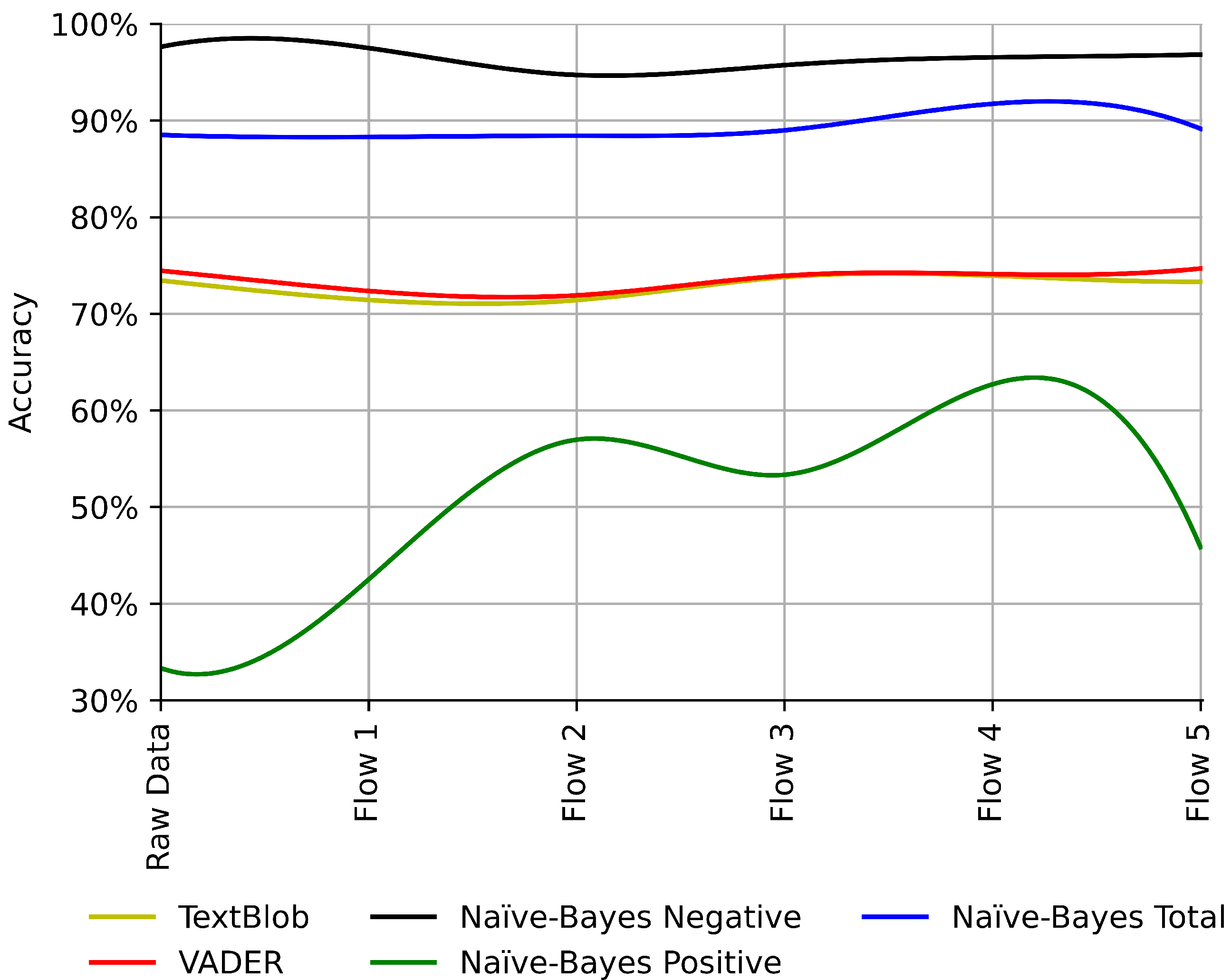
Given that naïve Bayes performed better than the other two classifiers in all cases, regardless of the pre-processing flow chosen, we opted to evaluate this classifier further. We started by testing naïve Bayes exclusively with negative tweets, then exclusively with positive tweets, and finally with all the tweets. The results of this additional evaluation are presented in

Table 5. Accuracy of the naïve Bayes classifier when testing, separately, with positive and negative tweets.

	Raw Data	Flow 1	Flow 2	Flow 3	Flow 4	Flow 5
Naïve Bayes Negative	95.44	93.52	90.63	91.63	93.03	92.09
Naïve Bayes Positive	41.48	54.15	55.11	52.02	59.15	48.10
Naïve Bayes Total	84.04	85.16	83.22	83.38	86.21	83.46

. Note that the results of testing exclusively with negative tweets are shown in the row titled “Naïve-Bayes Negative”, the results of testing exclusively with positive tweets are shown in the row titled “Naïve-Bayes Positive”, and the results of testing with all the tweets are shown on the row titled “Naïve-Bayes Total”. We also evaluated naïve Bayes when tested, separately, with the positive and negative tweets included in the gold standard. The results are presented in

Table 6. Accuracy of the naïve Bayes classifier when testing, separately, with the positive and negative tweets included in the gold standard.

	Raw Data	Flow 1	Flow 2	Flow 3	Flow 4	Flow 5
Naïve Bayes Negative	97.61	97.49	94.70	95.72	96.53	96.81
Naïve Bayes Positive	33.33	42.50	56.96	53.33	62.69	45.83
Naïve Bayes Total	88.50	88.28	88.42	88.98	91.72	89.14

. It should be observed that Flow 4 allows the naïve Bayes classifier to achieve its highest accuracy with the entire dataset, when tested exclusively with positive tweets and with all the tweets together—see Table 5. Additionally, Flow 4 allows the naïve Bayes classifier to achieve the highest accuracy with the gold standard, when tested exclusively with positive tweets and with all the tweets together—see Table 6.

Overall, Flow 4 appears to be the best pre-processing option. It allows the naïve Bayes classifier to achieve its highest accuracy with the entire dataset, when testing exclusively with positive tweets and all the tweets together—see Table 5. Additionally, it allows the naïve Bayes classifier to achieve the highest accuracy with the gold standard, when testing exclusively with positive tweets and all the tweets together—see Table 6. Our results can be summarised as follows:

• The importance of pre-processing: For each of the three classifiers evaluated, there is at least one pre-processing flow that increases its accuracy, regardless of the dataset employed for testing—the entire dataset or the gold standard—which confirms the benefits of pre-processing.
• Sensitivity: As it can be seen in Table 5 and Table 6, naïve Bayes positive achieves its worst accuracy overall without pre-processing. Additionally, naïve Bayes positive appears to be the most sensitive classifier to the pre-processing flows—that is, naïve Bayes positive is the classifier that improves its accuracy the most with the help of pre-processing. Indeed, Flow 4 enhances its accuracy significantly.
• Insensitivity: Both VADER and TextBlob achieve similar performance, and they seem to be insensitive to pre-processing—in the sense that pre-processing does not increase their accuracy considerably. According to Table 3 and Table 4, the variations in their accuracy, with and without any pre-processing, are minimal.
• Pre-processing loss: Naïve Bayes negative achieves the highest accuracy overall when tested with the entire dataset and the gold standard. However, such a high accuracy is achieved without any pre-processing.

Figure 9 and Figure 10 illustrate our results graphically.

The developers of VADER claim to have implemented a number of heuristics that people use to assess sentiment [75]. Such heuristics include, among others, pre-processing punctuation, capitalisation, degree modifiers—also called intensifiers, booster words, or degree adverbs—and dealing with the conjunction “but”, which typically signals a shift in sentiment polarity, with the sentiment of the text following the conjunction being the dominant part [75]. Hutto and Gilbert use the sentence “The food here is great, but the service is horrible” to show an example of mixed sentiment, where the latter half of the sentence dictates the overall polarity [75].

In other words, VADER performs its own text pre-processing, and this is likely to interfere with our flows. For instance, if we removed all the occurrences of the word “but” from the dataset while using Flow 4, because “but” is a stop-word, we would be disturbing VADER’s own pre-processing and, consequently, damaging its accuracy. Hence, VADER’s accuracy is not improved by Flow 4 or any other Flow where we remove stop-words. Unsurprisingly, VADER achieved its best performance with Flow 5, which is the only flow that does not remove stop-words. We can expect that TextBlob also performs its own pre-processing. After all, TextBlob and VADER are both off-the-shelf tools that implement solutions to the most common needs in sentiment analysis, without expecting their users to perform any pre-processing. Therefore, they are insensitive to our flows.

Table 5 and Table 6 show some high accuracy values for the naïve Bayes negative and total classifiers, which highlight the possibility of overfitting [78]. Clearly, overfitting is a fundamental issue in supervised machine learning, which prevents algorithms from performing correctly against unseen data. We need assurance that our classifier is not picking up too much noise. Thus, we have applied cross-validation [79]. We have separated our dataset into k subsets $(k=5)$, so that each time we test the classifier, one of the subsets is used as the test set, and the other $k-1$ subsets are put together to form the training set.

Table 7. Accuracy of the naïve Bayes negative and total classifiers after cross validation with the entire dataset.

	Raw Data	Flow 1	Flow 2	Flow 3	Flow 4	Flow 5
Naïve Bayes Negative	89.14	87.15	83.43	85.15	86.01	85.04
Naïve Bayes Total	78.24	79.11	77.02	77.05	80.14	77.07

shows the accuracy values after applying the k-fold cross validation.

While the accuracy is reduced by a small percentage after cross-validation, we still have Flow 4 as the best pre-processing option for Naïve Bayes Total—see Table 7. Of course, we are considering further training, testing, and validation with other datasets as part of our future work.

5. Conclusions

We have reviewed the available research on text pre-processing, focusing on how to improve the accuracy of sentiment analysis classifiers for social media. We have implemented several pre-processing components and evaluated various combinations of them. Our work has been tested with a collection of tweets obtained through Kaggle to quantitatively assess the accuracy improvements derived from pre-processing.

For each of the sentiment analysis classifiers evaluated in our study, there is at least one combination of pre-processing components that increases its accuracy, which confirms the importance and benefits of pre-processing. In the particular case of our naïve Bayes classifier, the experiments confirm that the order of the pre-processing components matters, and pre-processing can significantly improve its accuracy.

We have also discussed some challenges which require further research. Evidently, the accuracy of supervised learning classifiers depends heavily on the training data. Therefore, there is an opportunity to extend our work with new training samples. Our current results are promising and motivate further work in the future.

References

1. Liu, B. Sentiment Analysis and Subjectivity. Handb. Nat. Lang. Process. 2010, 2, 627–666. [Google Scholar]
2. Wiebe, J.M. Recognizing Subjective Sentences: A Computational Investigation of Narrative Text. Ph.D. Thesis, State University of New York at Buffalo, Buffalo, NY, USA, 1990. [Google Scholar]
3. Wiebe, J.M.; Bruce, R.F.; O’Hara, T.P. Development and Use of a Gold-Standard Data Set for Subjectivity Classifications. In Proceedings of the 37th Annual Meeting of the Association for Computational Linguistics on Computational Linguistics, College Park, MD, USA, 20–26 June 1999; Association for Computational Linguistics: Cambridge, MA, USA, 1999; pp. 246–253. [Google Scholar] [CrossRef]
4. Dave, K.; Lawrence, S.; Pennock, D.M. Mining the Peanut Gallery: Opinion Extraction and Semantic Classification of Product Reviews. In Proceedings of the 12th International Conference on World Wide Web, Budapest, Hungary, 20–24 May 2003; Association for Computing Machinery: New York, NY, USA, 2003; pp. 519–528. [Google Scholar] [CrossRef]
5. Pak, A.; Paroubek, P. Twitter as a Corpus for Sentiment Analysis and Opinion Mining. In Proceedings of the International Conference on Language Resources and Evaluation (LREC), Valletta, Malta, 17–23 May 2010; European Language Resources Association (ELRA): Valletta, Malta, 2010; pp. 1320–1326. [Google Scholar]
6. Solangi, Y.A.; Solangi, Z.A.; Aarain, S.; Abro, A.; Mallah, G.A.; Shah, A. Review on Natural Language Processing (NLP) and Its Toolkits for Opinion Mining and Sentiment Analysis. In Proceedings of the 5th International Conference on Engineering Technologies and Applied Sciences (ICETAS), Bangkok, Thailand, 22–23 November 2018; pp. 1–4. [Google Scholar] [CrossRef]
7. He, W.; Shen, J.; Tian, X.; Li, Y.; Akula, V.; Yan, G.; Tao, R. Gaining Competitive Intelligence from Social Media Data: Evidence from Two Largest Retail Chains in the World. Ind. Manag. Data Syst. 2015, 115, 1622–1636. [Google Scholar] [CrossRef]
8. Nguyen, T.H.; Shirai, K. Topic Modeling Based Sentiment Analysis on Social Media for Stock Market Prediction. In Proceedings of the 53rd Annual Meeting of the Association for Computational Linguistics and the 7th International Joint Conference on Natural Language Processing (Volume 1: Long Papers), Beijing, China, 26–31 July 2015; pp. 1354–1364. [Google Scholar]
9. Wang, H.; Can, D.; Kazemzadeh, A.; Bar, F.; Narayanan, S. A System for Real-Time Twitter Sentiment Analysis of 2012 U.S. Presidential Election Cycle. In Proceedings of the ACL 2012 System Demonstrations, ACL ’12, Jeju Island, Korea, 12–13 July 2012; Association for Computational Linguistics: Cambridge, MA, USA, 2012; pp. 115–120. [Google Scholar]
10. Palomino, M.; Taylor, T.; Göker, A.; Isaacs, J.; Warber, S. The Online Dissemination of Nature–Health Concepts: Lessons from Sentiment Analysis of Social Media Relating to Nature-Deficit Disorder. Int. J. Environ. Res. Public Health 2016, 13, 142. [Google Scholar] [CrossRef] [PubMed]
11. Velardi, P.; Stilo, G.; Tozzi, A.E.; Gesualdo, F. Twitter Mining for Fine-Grained Syndromic Surveillance. Artif. Intell. Med. 2014, 61, 153–163. [Google Scholar] [CrossRef]
12. Mantyla, M.V.; Graziotin, D.; Kuutila, M. The Evolution of Sentiment Analysis—A Review of Research Topics, Venues, and Top Cited Papers. Comput. Sci. Rev. 2018, 27, 16–32. [Google Scholar] [CrossRef]
13. Grefenstette, G. Tokenization. In Syntactic Wordclass Tagging; van Halteren, H., Ed.; Springer: Dordrecht, The Netherlands, 1999; Volume 9, pp. 117–133. [Google Scholar]
14. Saif, H.; Fernandez, M.; He, Y.; Alani, H. On Stopwords, Filtering and Data Sparsity for Sentiment Analysis of Twitter. In Proceedings of the International Conference on Language Resources and Evaluation (LREC), Reykjavik, Iceland, 26–31 May 2014; European Language Resources Association (ELRA): Reykjavik, Iceland, 2014; pp. 810–817. [Google Scholar]
15. Belew, R.K. Finding Out about: A Cognitive Perspective on Search Engine Technology and the WWW; Cambridge University Press: Cambridge, UK, 2000. [Google Scholar]
16. Jivani, A.G. A comparative study of stemming algorithms. Int. J. Comput. Technol. Appl. 2011, 2, 1930–1938. [Google Scholar]
17. Gesmundo, A.; Samardzic, T. Lemmatisation as a Tagging Task. In Proceedings of the 50th Annual Meeting of the Association for Computational Linguistics (Volume 2: Short Papers), Jeju Island, Korea, 8–14 July 2012; pp. 368–372. [Google Scholar]
18. Lyu, C.; Zhang, Y.; Ji, D. Joint Word Segmentation, Pos-Tagging and Syntactic Chunking. In Proceedings of the AAAI Conference on Artificial Intelligence, Phoenix, AR, USA, 12–17 February 2016; PKP Publishing Services Network: Burnaby, Canada, 2016; Volume 30. [Google Scholar]
19. Murthy, D. Twitter; Polity Press Cambridge: Cambridge, UK, 2018. [Google Scholar]
20. Kaggle Inc. Kaggle: Your Machine Learning and Data Science Community. 2021. Available online: https://www.kaggle.com/ (accessed on 29 July 2022).
21. Lowd, D.; Domingos, P. Naive Bayes Models for Probability Estimation. In Proceedings of the International Conference on Machine Learning, ICML ’05, Bonn, Germany, 7–11 August 2005; Association for Computing Machinery: New York, NY, USA, 2005; pp. 529–536. [Google Scholar] [CrossRef]
22. Burnham, J.F. Scopus Database: A Review. Biomed. Digit. Libr. 2006, 3, 1–8. [Google Scholar] [CrossRef]
23. Burgess, J.; Green, J. YouTube: Online Video and Participatory Culture; John Wiley & Sons: Hoboken, NJ, USA, 2018. [Google Scholar]
24. Caers, R.; De Feyter, T.; De Couck, M.; Stough, T.; Vigna, C.; Du Bois, C. Facebook: A Literature Review. New Media Soc. 2013, 15, 982–1002. [Google Scholar] [CrossRef] [Green Version]
25. Tankovska, H. Social Media Usage in the United Kingdom (UK)—Statistics & Facts. 2021. Available online: https://cybercrew.uk/blog/social-media-statistics-uk/ (accessed on 29 July 2022).
26. Tankovska, H. Leading Social Networks by Share of Website Visits in the United Kingdom (UK) as of January 2021; Statista Inc.: Hamburg, Germany, 2021. [Google Scholar]
27. Carnell, J.; Linwood, J.; Zawadzki, M. Creating a Search Engine with Lucene. In Professional Struts Applications: Building Web Sites with Struts, ObjectRelationalBridge, Lucene, and Velocity; Apress: Berkeley, CA, USA, 2003; pp. 237–266. [Google Scholar] [CrossRef]
28. Bastian, M.; Heymann, S.; Jacomy, M. Gephi: An Open Source Software for Exploring and Manipulating Networks. In Proceedings of the International AAAI Conference On web and Social Media, San Jose, CA, USA, 17–20 May 2009; Volume 3, pp. 361–362. [Google Scholar]
29. Sun, S.; Luo, C.; Chen, J. A Review of Natural Language Processing Techniques for Opinion Mining Systems. Inf. Fusion 2017, 36, 10–25. [Google Scholar] [CrossRef]
30. Jianqiang, Z.; Xiaolin, G. Comparison Research on Text Pre-processing Methods on Twitter Sentiment Analysis. IEEE Access 2017, 5, 2870–2879. [Google Scholar] [CrossRef]
31. Petz, G.; Karpowicz, M.; Fürschuß, H.; Auinger, A.; Stříteský, V.; Holzinger, A. Reprint of: Computational Approaches for Mining User’S Opinions on the Web 2.0. Inf. Process. Manag. 2015, 51, 510–519. [Google Scholar] [CrossRef]
32. Angiani, G.; Ferrari, L.; Fontanini, T.; Fornacciari, P.; Iotti, E.; Magliani, F.; Manicardi, S. A Comparison between Preprocessing Techniques for Sentiment Analysis in Twitter. In Proceedings of the 2nd International Workshop on Knowledge Discovery on the WEB (KDWeb), Cagliari, Italy, 8–10 September 2016; Armano, G., Bozzon, A., Cristani, M., Giuliani, A., Eds.; CEUR-WS.org: Cagliari, Italy, 2016. [Google Scholar]
33. Fornacciari, P.; Mordonini, M.; Tomaiuolo, M. A Case-Study for Sentiment Analysis on Twitter. In Proceedings of the Workshop From Objects to Agents, Naples, Italy, 17–19 June 2015; Napoli, C.D., Rossi, S., Staffa, M., Eds.; CEUR-WS.org: Naples, Italy, 2015; Volume 1382, pp. 53–58. [Google Scholar]
34. Połtyn, M. VADER Sentiment Analysis. 2020. Available online: https://pypi.org/project/vader-sentiment/ (accessed on 29 July 2022).
35. Loria, S. TextBlob Documentation. Release 0.15. 2018. Available online: https://textblob.readthedocs.io/en/dev/index.html (accessed on 29 July 2022).
36. Aker, A.; Petrak, J.; Sabbah, F. An Extensible Multilingual Open Source Lemmatizer. In Proceedings of the International Conference Recent Advances in Natural Language Processing, Varna, Bulgaria, 2–8 September 2017; ACL: Varna, Bulgaria, 2017; pp. 40–45. [Google Scholar]
37. Joshi, A.; Bhattacharyya, P.; Carman, M.J. Automatic Sarcasm Detection: A Survey. ACM Comput. Surv. 2017, 50, 1–22. [Google Scholar] [CrossRef]
38. Pontiki, M.; Galanis, D.; Papageorgiou, H.; Manandhar, S.; Androutsopoulos, I. Semeval-2015 Task 12: Aspect Based Sentiment Analysis. In Proceedings of the International Workshop on Semantic Evaluation (SemEval 2015), Denver, CO, USA, 4–5 June 2015; pp. 486–495. [Google Scholar]
39. Nakov, P.; Ritter, A.; Rosenthal, S.; Sebastiani, F.; Stoyanov, V. Semeval-2016 Task 4: Sentiment Analysis in Twitter. In Proceedings of the 10th International Workshop on Semantic Evaluation (SemEval-2016), San Diego, CA, USA, 16–17 June 2016; pp. 31–41. [Google Scholar]
40. Van Rijsbergen, C. Information Retrieval: Theory and Practice. In Proceedings of the Joint IBM/University of Newcastle upon Tyne Seminar on Data Base Systems, Newcastle upon Tyne, UK, 4–7 September 1979; pp. 1–14. [Google Scholar]
41. Wikimedia Foundation, Inc. List of Emoticons. 2021. Available online: https://en.wikipedia.org/wiki/List_of_emoticons (accessed on 29 July 2022).
42. Internet Slang Dict. Acronym List. 2021. Available online: http://www.noslang.com/dictionary/ (accessed on 29 July 2022).
43. Python Software Foundation. PyEnchant. 2021. Available online: https://pypi.org/project/pyenchant/ (accessed on 29 July 2022).
44. Bounabi, M.; Moutaouakil, K.E.; Satori, K. A Comparison of Text Classification Methods using Different Stemming Techniques. Int. J. Comput. Appl. Technol. 2019, 60, 298–306. [Google Scholar] [CrossRef]
45. Appen Ltd. Datasets Resource Center. 2021. Available online: https://appen.com/open-source-datasets/ (accessed on 29 July 2022).
46. Flint, J. Republican Debate Audience Was the Biggest Ever for a Nonsports Cable Event. The Wall Street Journal. 2015. Available online: https://www.wsj.com/articles/republican-debate-audience-was-the-biggest-ever-for-a-nonsports-cable-event-1438992539 (accessed on 29 July 2022).
47. Kaggle. First GOP Debate Twitter Sentiment. 2021. Available online: https://www.kaggle.com/crowdflower/first-gop-debate-twitter-sentiment (accessed on 29 July 2022).
48. Palomino, M.; Oakes, M.; Wuytack, T.A. Concept suggestion engine for professional multimedia archives. Res. Comput. Sci. Adv. Comput. Sci. Eng. 2009, 42, 29–40. [Google Scholar]
49. Mueller, A. WordCloud for Python Documentation. 2020. Available online: https://amueller.github.io/word_cloud/ (accessed on 29 July 2022).
50. Tait, A. Why Are Online Jokes Funnier without Punctuation and Capital Letters? The New Statesman. 2016. Available online: https://www.newstatesman.com/science-tech/2016/10/why-are-online-jokes-funnier-without-punctuation-and-capital (accessed on 29 July 2022).
51. Kim, K. An Improved Semi-Supervised Dimensionality Reduction Using Feature Weighting: Application to Sentiment Analysis. Expert Syst. Appl. 2018, 109, 49–65. [Google Scholar] [CrossRef]
52. Symeonidis, S.; Effrosynidis, D.; Arampatzis, A. A Comparative Evaluation of Pre-Processing Techniques and their Interactions for Twitter Sentiment Analysis. Expert Syst. Appl. 2018, 110, 298–310. [Google Scholar] [CrossRef]
53. Manning, C.D.; Raghavan, P.; Schütze, H. Introduction to Information Retrieval; Cambridge University Press: Cambridge, UK, 2008. [Google Scholar]
54. Sinka, M.P.; Corne, D. Evolving Better Stoplists for Document Clustering and Web Intelligence. In Design and Application of Hybrid Intelligent Systems; IOS Press: Amsterdam, The Netherlands, , 2003; pp. 1015–1023. [Google Scholar]
55. Makrehchi, M.; Kamel, M.S. Extracting Domain-Specific Stopwords for Text Classifiers. Intell. Data Anal. 2017, 21, 39–62. [Google Scholar] [CrossRef]
56. Bird, S.; Klein, E.; Loper, E. Natural Language Processing with Python: Analyzing Text with the Natural Language Toolkit; O’Reilly Media, Inc.: Sebastopol, CA, USA, 2009. [Google Scholar]
57. Taggart, C. New Words for Old: Recycling our Language for the Modern World; Michael O’Mara Books: London, UK, 2015; p. 192. [Google Scholar]
58. Wang, H.; Castanon, J.A. Sentiment Expression via Emoticons on Social Media. In Proceedings of the 2015 IEEE International Conference on Big Data (Big Data), Santa Clara, CA, USA, 29 October–1 November 2015; pp. 2404–2408. [Google Scholar]
59. Fernández-Gavilanes, M.; Juncal-Martínez, J.; García-Méndez, S.; Costa-Montenegro, E.; González-Castaño, F.J. Creating Emoji Lexica from Unsupervised Sentiment Analysis of Their Descriptions. Expert Syst. Appl. 2018, 103, 74–91. [Google Scholar] [CrossRef]
60. Shah, N.; Rohilla, S. emot: Open Source Emoticons and Emoji Detection Library; GitHub, Inc.: San Francisco, CA, USA, 2022; Available online: https://github.com/NeelShah18/emot (accessed on 29 July 2022).
61. Satapathy, R.; Guerreiro, C.; Chaturvedi, I.; Cambria, E. Phonetic-based Microtext Normalization for Twitter Sentiment Analysis. In Proceedings of the IEEE International Conference On Data Mining Workshops, New Orleans, LA, USA, 18–21 November 2017; pp. 407–413. [Google Scholar]
62. Palomino, M.; Grad, D.; Bedwell, J. GoldenWind at SemEval-2021 Task 5: Orthrus-An Ensemble Approach to Identify Toxicity. In Proceedings of the International Workshop on Semantic Evaluation (SemEval-2021), Bangkok, Thailand, 5–6 August 2021; Association for Computational Linguistics: Stroudsburg, PA, USA, 2021; pp. 860–864. [Google Scholar]
63. Verma, R. SMS Slang Translator; GitHub, Inc.: San Francisco, CA, USA, 2022. [Google Scholar]
64. Mullen, T.; Malouf, R. A Preliminary Investigation into Sentiment Analysis of Informal Political Discourse. In Proceedings of the AAAI Spring Symposium: Computational Approaches to Analyzing Weblogs, Menlo Park, CA, USA, 27–29 March 2006; pp. 159–162. [Google Scholar]
65. Carley, K.M.; Columbus, D.; Landwehr, P. AutoMap User’s Guide 2013; Technical Report CMU-ISR-13-105; Carnegie Mellon University, School of Computer Science, Institute for Software Research: Pittsburgh, PA, USA, 2013. [Google Scholar]
66. Barrus, T. Pure Python Spell Checker Based on Work by Peter Norvig. 2022. Available online: https://pypi.org/project/pyspellchecker/ (accessed on 29 July 2022).
67. Yujian, L.; Bo, L. A normalized Levenshtein distance metric. IEEE Trans. Pattern Anal. Mach. Intell. 2007, 29, 1091–1095. [Google Scholar] [CrossRef]
68. Pradana, A.W.; Hayaty, M. The Effect of Stemming and Removal of Stopwords on the Accuracy of Sentiment Analysis on Indonesian-Language Texts. Kinet. Game Technol. Inf. Syst. Comput. Netw. Comput. Electron. Control 2019, 4, 375–380. [Google Scholar] [CrossRef]
69. Duong, H.T.; Nguyen-Thi, T.A. A Review: Preprocessing Techniques and Data Augmentation for Sentiment Analysis. Comput. Soc. Netw. 2021, 8, 1–16. [Google Scholar] [CrossRef]
70. Haynes, C.; Palomino, M.A.; Stuart, L.; Viira, D.; Hannon, F.; Crossingham, G.; Tantam, K. Automatic Classification of National Health Service Feedback. Mathematics 2022, 10, 983. [Google Scholar] [CrossRef]
71. Loria, S. TextBlob: Simplified Text Processing. 2020. Available online: https://textblob.readthedocs.io/en/dev/ (accessed on 29 July 2022).
72. Palomino, M.A.; Varma, A.P.; Bedala, G.K.; Connelly, A. Investigating the Lack of Consensus Among Sentiment Analysis Tools. In Human Language Technology. Challenges for Computer Science and Linguistics; Vetulani, Z., Paroubek, P., Kubis, M., Eds.; Springer International Publishing: Cham, Switzerland, 2020; pp. 58–72. [Google Scholar]
73. De Smedt, T.; Daelemans, W. Pattern for python. J. Mach. Learn. Res. 2012, 13, 2063–2067. [Google Scholar]
74. Perkins, J. Python 3 Text Processing with NLTK 3 Cookbook; Packt Publishing Ltd.: Birmingham, UK, 2014. [Google Scholar]
75. Hutto, C.J.; Gilbert, E. VADER: A Parsimonious Rule-Based Model for Sentiment Analysis of Social Media Text. In Proceedings of the 8th International AAAI Conference on Weblogs and Social Media, Ann Arbor, MI, USA, 1–4 June 2014; The AAAI Press: Ann Arbor, MI, USA, 2014; pp. 216–225. [Google Scholar]
76. Ligthart, A.; Catal, C.; Tekinerdogan, B. Analyzing the Effectiveness of Semi-Supervised Learning Approaches for Opinion Spam Classification. Appl. Soft Comput. 2021, 101, 107023. [Google Scholar] [CrossRef]
77. Zhang, H.; Su, J. Naive Bayesian Classifiers for Ranking. In European Conference on Machine Learning; Springer: Berlin/Heidelberg, Germany, 2004; pp. 501–512. [Google Scholar]
78. Ying, X. An Overview of Overfitting and Its Solutions. J. Phys. Conf. Ser. 2019, 1168, 022022. [Google Scholar] [CrossRef]
79. Wong, T.T.; Yeh, P.Y. Reliable Accuracy Estimates from k-Fold Cross Validation. IEEE Trans. Knowl. Data Eng. 2020, 32, 1586–1594. [Google Scholar] [CrossRef]
Figure 1. Distribution of tweets per hour. Tweets were collected from 6 August 2015 at 17:44:53 to 7 August 2015 at 10:12:32.
Applsci 12 08765 g001
Figure 2. Distribution of positive, negative, and neutral tweets in the experimental dataset per hour. The tweets included in the plot are those annotated with a high confidence sentiment value.
Applsci 12 08765 g002
Figure 3. Dataset word cloud based on TF-IDF to determine the most characteristic words.
Applsci 12 08765 g003
Figure 4. Flow 1: Reference flow.
Applsci 12 08765 g004
Figure 5. Flow 2.
Applsci 12 08765 g005
Figure 6. Flow 3.
Applsci 12 08765 g006
Figure 7. Flow 4.
Applsci 12 08765 g007
Figure 8. Flow 5.
Applsci 12 08765 g008
Figure 9. Accuracy of the classifiers on the entire dataset.
Applsci 12 08765 g009
Figure 10. Accuracy of the classifiers on the gold standard.
Applsci 12 08765 g010