Redundant Robot with Pneumatic Artificial Muscles for Rehabilitation Works Using Iterative Learning Control

Abstract

This study aims to develop a multi-functional robotic arm with a multi-degree of freedom using a pneumatic artificial muscle cylinder as the main actuator, with a wearable function. While wearing the robotic arm, it has four degrees of freedom and can be used as an upper limb rehabilitation aid to perform rehabilitation exercise tasks. The rotating axes are driven by pneumatic artificial muscle cylinders to ensure the safety and flexibility of the robot interaction. By integrating multiple pneumatic control valves and sensors with embedded interface cards, the control of pneumatic artificial muscle cylinders is performed, and the rehabilitation trajectory commands are planned through the kinematics of the robotic arm, and a closed-loop control system is established to enable the robotic arm to achieve the task of rehabilitation trajectory tracking. In the single-axis robotic arm controller experiment, it was found that the LMS-PID is superior to the conventional PID control method. In the control experiment of the robotic arm under the multi-axis recovery trajectory, the result showed that the training of drawing a circle on the wall could be successfully planned. In the multi-axis robotic tracking experiment under the rehabilitation trajectory, the result showed that the RMSE of the tracking trajectory decreased to 0.2444 and 0.2853. In the robotic arm joining/loading experiment, it was shown that the method of this study can withstand some loading effects. Moreover, this study introduces iterative learning control to improve the non-linear compensation and phase lag problems of the PID controller so that the robot arm can have a certain tracking accuracy under the round-trip robust trajectory.

1. Introduction

The application of robotic arms is widespread, including in industrial manufacturing automation applications [1,2], military security, disaster prevention and explosion removal [3], medical rehabilitation [4,5,6], and home entertainment [7]. Robotic arms have been applied in many fields. The medical rehabilitation robots mentioned above have been important research topics. 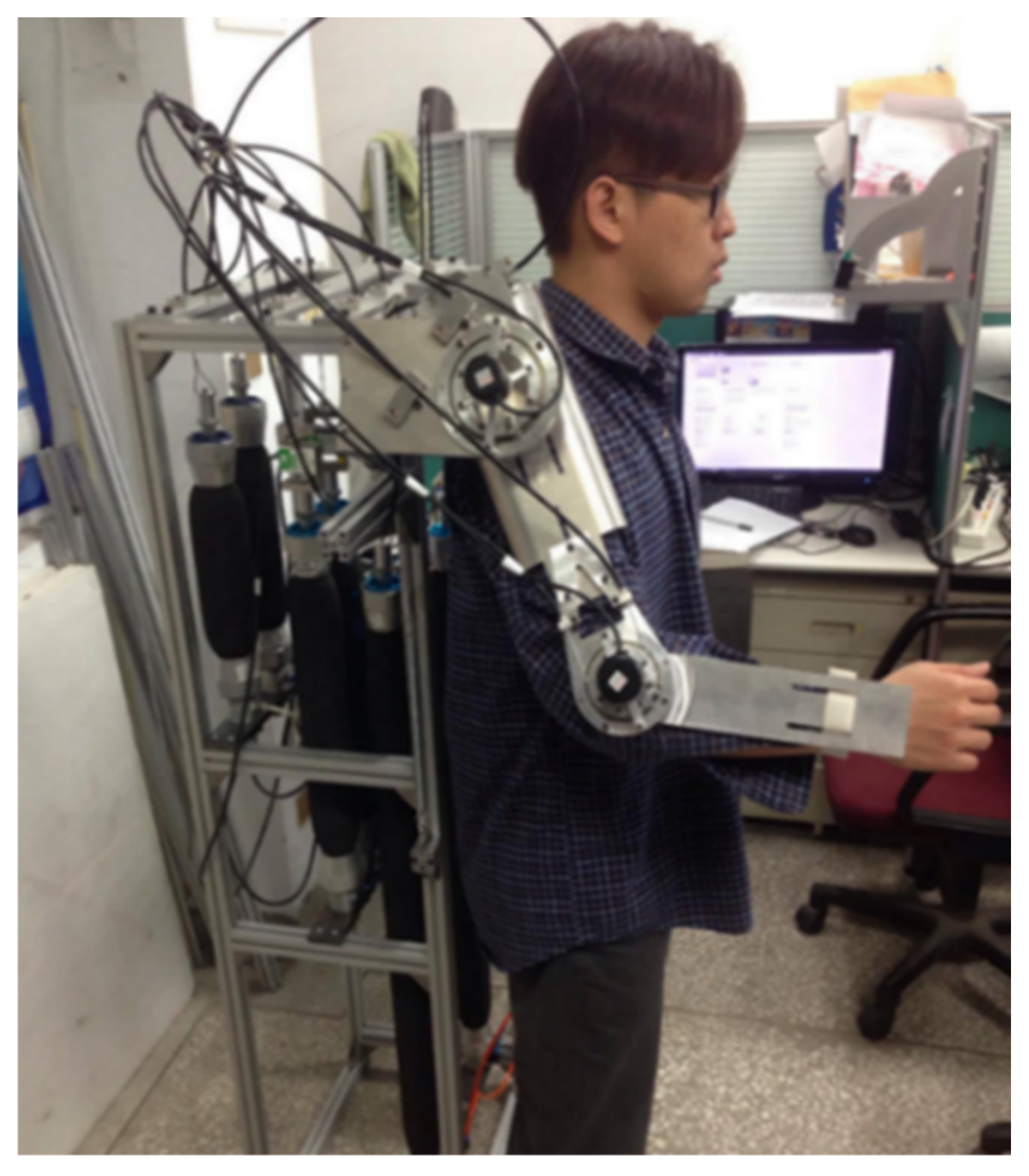Patients with physical movement disabilities caused by accidents, surgery after injury or brain injury, stroke, etc., are unable to take care of themselves in daily life and need to be cared for long-term by others [8]. Thus, this study aims to develop a multi-functional robotic arm and design a multi-degree of freedom robotic arm for patients who cannot lift their upper limbs by themselves and need to be assisted by devices for rehabilitation training. It is designed as a human-shaped exoskeleton with a wearable function so that the patient can perform rehabilitation exercises for the upper limbs with the help of the robotic arm while wearing it.

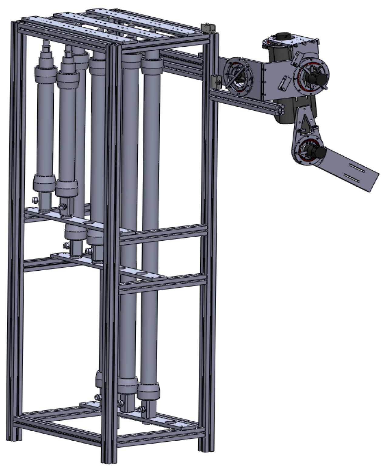
To design an upper limb wearable robotic arm, it is necessary to consider the design process and validation issues [9,10]. An upper limb wearable robotic arm is an assistive device in direct contact with the user’s body, and its safety and flexibility are very important. Rehabilitation tasks require stability and comfort. At present, most robotic arms are driven by motors, where the advantages of motors are high-speed response time, high precision, and high linearity, but because of the direct action on the rotary axis, improper control will make patients feel pain and cause secondary injury. Thus, Festo’s pneumatic muscle cylinder is used as the actuator in this study. In comparison with motors or pneumatic cylinder actuators, it has the following advantages: slower reaction speed, limited movement stroke, and higher output force. Additionally, flexible material is used to make the pneumatic artificial muscle cylinder, and the rotation of the rotary axis is a little flexible during the robotic arm’s rehabilitation tasks. Hence, it is more suitable for human–computer interaction robotic arm development than rigid material actuators such as motors and pneumatic cylinders.

Pneumatic artificial muscle (PAM) was first designed in 1961 by Joseph L. McKibben, an American physicist, as his daughter was suffering from osteomyelitis and McKibben was looking for an actuator with flexible material that could be used as a prosthesis [11]. McKibben invented PAM in order to obtain a material that was flexible and could be used as an actuator for a prosthesis, and thus, PAM was also called McKibben muscle [12]. From the perspective of PAM and biological muscle, PAM has the advantages of higher output force, high energy-conversion efficiency, faster dynamic characteristics, compact structure, light weight, flexibility, easy control of extension position through pressure valve control, and less heat, noise, and harmful substances during operation. On the other hand, the disadvantages are that the displacement change of PAM is time-varying and non-linear compared to the input pressure, and there is some friction between the inner elastic rubber tube and the outer fiber mesh of PAM when the displacement change occurs due to the internal pressure change, thus causing a hysteresis phenomenon [13,14].

In recent years, the German Festo team has been developing the application of PAM in robotics. The ZAR5, developed by the Festo team, uses PAM as an actuator, and its mechanism consists of a rotatable base, two upper limb arms, and a total of ten fingers on both hands. By controlling the flow valve to change the air flow in the pneumatic artificial muscles, it can perform the action of bending the fingers with the arms together and can track the action of simulated human hands [15]. A UK-based shadow company also designed a bionic arm using PAMs, with each group of PAMs installed in the same position as the corresponding muscles of the human arm, which can realize the same bending elbow and arm forward and extension movements as human hands [16]. Tondu et al. [17] published a seven-degrees-of-freedom humanoid robotic arm with PAM as the actuator to drive each axis of the arm in remote control mode, allowing the arm to perform the task of picking up and dropping objects. Caldwell et al. [18] designed an exoskeleton device for upper limb and lower limb rehabilitation with seven degrees of freedom for the upper limb exoskeleton and five degrees of freedom for the lower limb exoskeleton, which is driven by a PAM. The upper limb exoskeleton is equipped with a torque sensor at the end of the hand, which can sense the force signal applied at the end of the hand and use the force signal to achieve the desired movement position of the patient through control.

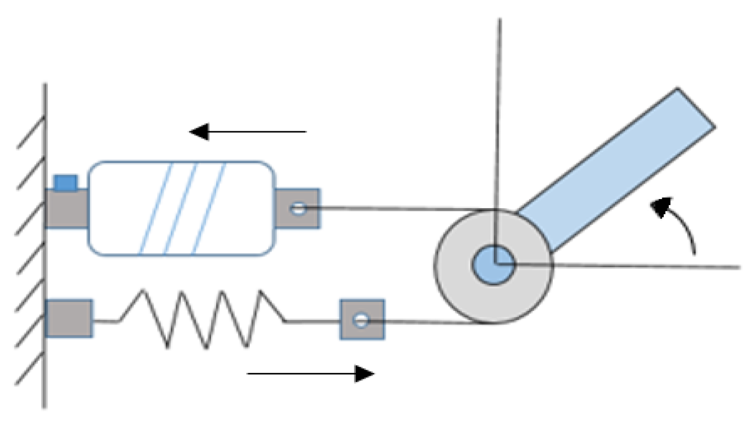
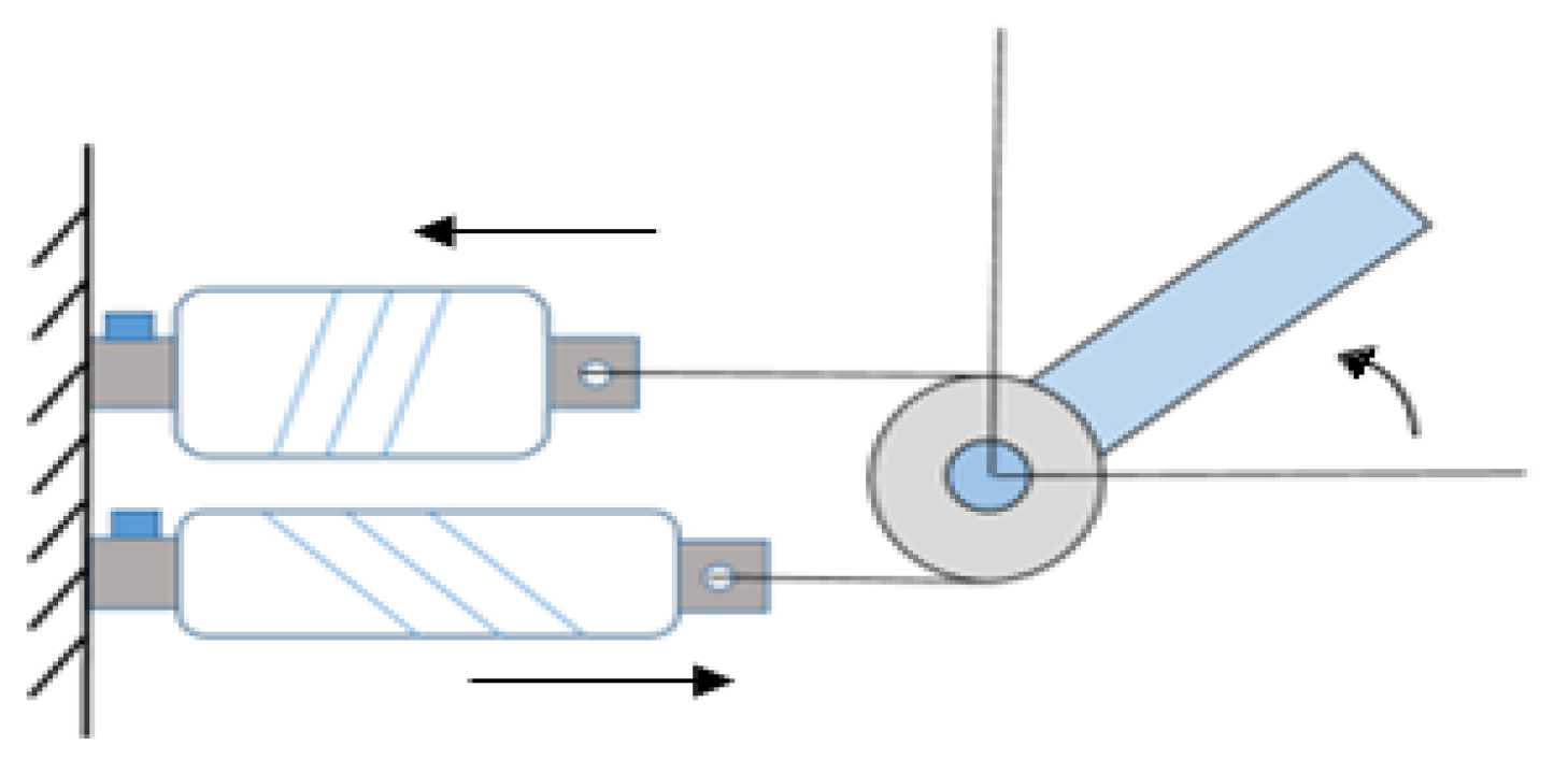
PAMs are applied to control robotic arms, which can be generally classified as single PAM control or dual PAMs operating in linear or rotary motion; the use of pneumatic control valves is also different from pressure control valves or flow-control flow servo valves. Minh et al. [19] used a proportional flow-control PAM, but because the PAM produced hysteresis during operation, the hysteresis was modeled by isometric, isobaric, and isotropic experiments to perform feed-forward compensation so that the system could achieve better control results. Shen [20] proposed using sliding mode control (SMC) to control the linear motion of a proportional flow servo valve with dual PAMs, and established a nonlinear model of the PAMs, with ideal gas equation and air flow equation to derive the relationship between the control command parameters and the dual PAMs, and designed the sliding plane to calculate the control commands through the equivalent control law and switching control law to control the system. Andrikopoulos et al. [21] used a nonlinear proportional–integral–derivative (PID) structure to simplify the modeling process and provide pneumatic artificial muscles to compensate for nonlinear hysteresis phenomena and increase the robustness of the system.

In order to improve the control accuracy of the trajectory tracking, this study uses iterative learning control. The initial idea of iterative learning control was to make a relevant correction to the control of mechanical motion through the implementation error in the mechanical system, but the analysis of learning control was still insufficient at that time [22]. Arimoto et al. [23] proposed a learning algorithm called the PID-type, which can guarantee the convergence of the system without initial error and specially defined norm limits. Since then, different definitions of iterative learning control and modified learning algorithms have been proposed; these learning algorithms require several iterations to achieve a certain control accuracy [24,25]. Kurek and Zaremba [26] proposed a theoretical algorithm that can adjust the control error to zero in just one learning session, but this method is obtained from the system state generated by the new control input. Geng et al. [27] introduced iterative learning control (ILC) with a two-dimensional system theory and introduced a suitable mathematical model to clearly describe the dynamics of the control system and the learning process behavior. However, their proposed method must be full-state feedback and can only be applied to first-order systems. They also applied two-dimensional system theory to propose an iterative learning control method for continuous-time and discrete-time systems [28,29].

To sum up, the purpose of this study is to develop a robotic arm with a rehabilitation function and to conduct various experimental validations. This study involves designing a single-axis robotic arm controller, a robotic arm on a multi-axis recovery trajectory, a multi-axis robotic tracking experiment on a rehabilitation trajectory, and a robotic arm joining/loading experiment.

2. Materials and Methods

2.1. Experimental Design and Introduction

2.1.1. Design of Robotic Arm

The structure and movement patterns of the human upper limbs are introduced prior to designing the upper limb wearable robotic arm; the human upper limb can be divided into three major parts, including the upper arm, forearm, and hand end, and the main joints are formed by the shoulder, elbow, and wrist joints. The complete structure of the robotic arm designed in this research is shown in Figure 1, which is divided into three parts: shoulder, elbow, and wrist; the shoulder is designed to imitate the movement of the human shoulders and has three degrees of freedom, while the elbow is designed to consider the user’s safety while wearing it, and only one degree of freedom is designed. Its operation is shown in Figure 2.

In this study, the mechanism of each axis of the robotic arm was designed with reference to the design of the rehabilitative arm in [9], and its operation was simulated after considering the cost and light weight. The range of rotation of the robotic arm must not only be smaller than the angle of human joints, but also the first and third axis of rotation must be limited to ensure that the mechanism will not cause excessive collision with the human body while wearing the arm. The range of rotation angles between the human joints and the robot arm is shown in

Table 1. Motion range of human joints and design of the rotational axis of the robotic arm [9].

Operation	Human Arm (Degree)	Robotic Arm (Rotary Axis)	Robotic Arm (Degree)
Shoulder (Adduction~Abduction)	−48~134	1st axis	−5~45
Shoulder (Extension~Flexion)	−61~188	2nd axis	−10~100
Shoulder (Horizontal adduction~Horizontal abduction)	−34~97	3rd axis	−10~20
Elbow (Extension~Flexion)	0~142	4th axis	0~100

. The PAM is used as the actuator and is fixed to the pulley of the robotic arm through a steel cable that leads to the brake pipe. When the PAM moves, it can drive the rotating axis of the robot arm. In this study, seven PAMs were used to drive the rotating axis, and the PAMs were fixed to an aluminum frame with the robotic arm, instead of wearing them completely on the human body, as shown in Figure 3. For the rehabilitation of the human body, it can reduce the unnecessary mechanical load on human joints, as shown in Figure 3.

2.1.2. Robotic Arm’s Forward Kinematics

To analyze the motion of the robot arm, the coordinate system relationship of the robot arm must be defined first. The homogeneous transformation matrix proposed by Denavit and Hartenberg (the D-H method) is commonly used to analyze the coordinate system transformation between each axis of the robot arm. In this study, the robotic arm has four degrees of freedom, and the relationship between the coordinate systems is shown in Figure 4. The coordinate system ${\left(XYZ\right)}_i$$i=0\dots N$ on each rotary axis is defined according to the D-H method and the parameters recorded in the D-H parameter table, as shown in

Table 2. D-H parameter table for four-degrees-of-freedom robot arm.

${\mathit{\theta }}_{\mathit{i}} \left(\mathbf{Degree}\right)$	d (Meter)	a (Meter)	α (Degree)
${\theta }_1-90$	0	0	90
${\theta }_2+90$	0	0	−90
${\theta }_3$	0.29	0	90
${\theta }_4+90$	0	0.27	0

.

As an example in this paper, the four-degrees-of-freedom robotic arm is defined as a matrix with the coordinate conversion relationship, and the D-H homogenous transform matrix ${}^{i}A{}_{i+1}$ is shown in (1):

$$\begin{array}{ll}{}^{i}A{}_{i+1}& =Rot(Z_{i-1,}{\theta }_i)\times Trans(0,0,d_i)\times Trans(a_i,0,0)\times Rot(X_{i-1,}{a}_i)\\ & =\left[\begin{array}{cccc}\cos ({\theta }_i)& -\sin ({\theta }_i)\cos ({\alpha }_i)& \sin ({\theta }_i)\sin ({\alpha }_i)& a_i\cos ({\theta }_i)\\ \sin ({\theta }_i)& \cos ({\theta }_i)\cos ({\alpha }_i)& -\cos ({\theta }_i)\sin ({\alpha }_i)& a_i\sin ({\theta }_i)\\ 0& \sin ({\alpha }_i)& \cos ({\alpha }_i)& d_i\\ 0& 0& 0& 1\end{array}\right]\end{array}$$

(1)

where:

• ${\theta }_i:Z_{i-1}$-axis rotation angle,
• $d_i:Z_{i-1}$-direction, distance of translation,
• $a_i:X_{i-1}$-direction, distance of translation,
• ${\alpha }_i:X_{i-1}$-axis rotation angle.

By using (1), the homogeneous transformation matrix of each joint is constructed, and the transformation matrix of each joint is multiplied in order to calculate the transformation relationship between the end-point coordinate system and the origin (P₀), as in Equation (2):

$$P_0={}^{0}A{}_1{}^{1}A{}_2{}^{2}A{}_3{}^{3}A{}_4{P}_4$$

(2)

where:

$${}^{0}A{}_1=\left[\begin{array}{cccc}\cos \left({\theta }_1\right)& 0& \sin \left({\theta }_1\right)& 0\\ \sin \left({\theta }_1\right)& 0& -\cos ({\theta }_1)& 0\\ 0& 1& 0& 0\\ 0& 0& 0& 1\end{array}\right]$$

(3)

$${}^{1}A{}_2=\left[\begin{array}{cccc}\cos \left({\theta }_2\right)& 0& -\sin \left({\theta }_2\right)& 0\\ \sin \left({\theta }_2\right)& 0& \cos ({\theta }_2)& 0\\ 0& -1& 0& 0\\ 0& 0& 0& 1\end{array}\right]$$

(4)

$${}^{2}A{}_3=\left[\begin{array}{cccc}\cos \left({\theta }_3\right)& 0& \sin \left({\theta }_3\right)& 0\\ \sin \left({\theta }_3\right)& 0& -\cos ({\theta }_3)& 0\\ 0& 1& 0& d_3\\ 0& 0& 0& 1\end{array}\right]$$

(5)

$${}^{3}A{}_4=\left[\begin{array}{cccc}\cos \left({\theta }_4\right)& -\sin \left({\theta }_4\right)& 0& a_4\cos \left({\theta }_4\right)\\ \sin \left({\theta }_4\right)& \cos \left({\theta }_4\right)& 0& a_4\sin \left({\theta }_4\right)\\ 0& 0& 1& 0\\ 0& 0& 0& 1\end{array}\right]$$

(6)

To calculate the end position vector of the robot arm, substitute into Equation (2) to obtain the coordinates of its end, as shown in Equation (7):

$$\left[\begin{array}{c}x\\ y\\ z\\ 1\end{array}\right]=\left[\begin{array}{c}-a_4\cos ({\theta }_4)\left(\sin \left({\theta }_1\right)\sin \left({\theta }_3\right)-\cos \left({\theta }_1\right)\cos \left({\theta }_2\right)\cos \left({\theta }_3\right)\right)-d_3\cos \left({\theta }_1\right)\sin \left({\theta }_2\right)-a_4\cos \left({\theta }_1\right)\sin \left({\theta }_2\right)\sin \left({\theta }_4\right)\\ a_4\cos ({\theta }_4)\left(\cos \left({\theta }_1\right)\sin \left({\theta }_3\right)+\cos \left({\theta }_2\right)\cos \left({\theta }_3\right)\sin \left({\theta }_1\right)\right)-d_3\sin \left({\theta }_1\right)\sin \left({\theta }_2\right)-a_4\sin \left({\theta }_1\right)\sin \left({\theta }_2\right)\sin \left({\theta }_4\right)\\ d_3\cos \left({\theta }_2\right)+a_4\cos \left({\theta }_2\right)\sin \left({\theta }_4\right)+a_4\cos \left({\theta }_3\right)\cos \left({\theta }_4\right)\sin \left({\theta }_2\right)\\ 1\end{array}\right]$$

(7)

2.1.3. Robotic Arm’s Inverse Kinematics

Consider a robotic joint with degrees of freedom at any given time, and the number of degrees of freedom required to perform a task in the Cartesian coordinate system. Then, the joint angle vector of the robotic arm can be defined as Equation (8):

$$\theta \left(t\right)=\left[{\theta }_{1,}{\theta }_{2,}\dots {\theta }_n\right]\in R^n$$

(8)

The end position vector of the robot arm describing the task can be defined as Equation (9):

$$r\left(t\right)=\left[x_{1,}{x}_{2,}\dots x_n\right]\in R^m$$

(9)

Inverse kinematics is to invert the angle and angular velocity solution of each joint according to the trajectory of the end in the Cartesian coordinates. Thus, the basic task of the robot arm is defined as follows: the end of the robotic arm must achieve the required trajectory in the Cartesian coordinates; if the default trajectory is expressed as a time series, the basic task of the robotic arm can be expressed as finding the minimum value of the correct position of the end, as in Equation (10):

$$Minimize{\left(r\left(t\right)-r_{ref}\left(t\right)\right)}^T\left(r\left(t\right)-r_{ref}\left(t\right)\right)$$

(10)

Normally, the forward kinematic relation is non-linear and it is difficult to obtain the inverse analytical relation; therefore, to obtain the inverse relation, it is generally obtained by differentiation.

$$\dot{r}\left(t\right)=J\left(\theta \left(t\right)\right)\dot{\theta }\left(t\right)$$

(11)

where $J\left(\theta \left(t\right)\right)$ is the Jacobian matrix, which is used to describe the velocity vector relationship between the Cartesian coordinates of the robotic arm end point and the joint angle, as shown in Equation (12).

$$J\left(\theta \left(t\right)\right)=\frac{\partial f\left(\theta \left(t\right)\right)}{\partial \theta \left(t\right)}$$

(12)

When the degrees of freedom of the robotic arm are the same as those required for the preset task $\left(n=m\right)$, and $\left|J\right|\ne 0$, then the inverse kinematics can be obtained from Equation (13), where $J^{-1}=\frac{adj(J)}{\left|J\right|}$.

$$\dot{\theta }\left(t\right)=J^{-1}\left(\theta \left(t\right)\right)\dot{r}\left(t\right)$$

(13)

When the degrees of freedom of the robotic arm are greater than the degrees of freedom required by the default task $\left(n>m\right)$, then the robotic arm is a redundant robot arm for this task. For the inverse kinematics of the robotic arm with redundant degrees of freedom, one of the particular solutions can be obtained by the Moore–Penrose pseudoinverse; when using the Moore–Penrose pseudoinverse to calculate the inverse kinematics, a particular solution can be obtained such that $\Vert \dot{\theta }\Vert$ has a minimum at time $t_k\in \left[t_{0,}{t}_f\right]$. If $rank[J\left(\theta \left(t_k\right)\right)]=m$ is established at $t_k\in \left[t_{0,}{t}_f\right]$, then the pseudoinverse of the Jacobian matrix can be defined as in Equation (14):

$$J^{+}\left(\theta \left(t_k\right)\right)=J{\left(\theta \left(t_k\right)\right)}^T\left(J\left(\theta \left(t_k\right)\right)\right)J{\left({\left(\theta \left(t_k\right)\right)}^T\right)}^{-1}$$

(14)

The particular solution of the inverse kinematics can be expressed as Equation (15):

$$\dot{\theta }\left(t_k\right)=J^{+}\left(\theta \left(t_k\right)\right)\dot{r}\left(t_k\right)$$

(15)

At some time $t_s\in \left[t_{0,}{t}_f\right]$ does not fulfill $Rank\left[J\left(\theta \left(t_k\right)\right)\right]=m$, i.e., when $Rank\left[J\left(\theta \left(t_k\right)\right)\right]<m$, the robot arm is at the singularity point, and near the singularity point, the correct solution cannot be obtained using Equation (14) because of $\left|J\left(\theta \left(t_s\right)\right)J{\left(\theta \left(t_s\right)\right)}^T\right|=0$. Thus, the trajectory should be planned to avoid singularities to prevent the robotic arm from being in an odd attitude.

2.1.4. Hardware and Software Introduction

In this study, the mechanical and electrical system architecture of the robotic arm uses a PC and a real-time monitoring system as the control side. The host side is the Windows operating system, and the programming of the real-time monitoring system side is communicated by LabVIEW software and the embedded controller myRIO. The control process is that the host gives the control command to each rotary axis of the robotic arm, with a real-time monitoring system and embedded controller to control the corresponding pneumatic valve of each axis, through the rotary encoder and pressure sensor feedback information, in order to perform the task of tracking.

The pneumatic artificial muscle cylinder is a tensioner produced by Festo (Esslingen, Germany, MAS-40-XXXXN-AA-MC-O-ER-BG), which uses pneumatic pressure as a power source to imitate the stretching motion of human muscles. Its structure is composed of a contraction system and two connectors, in which the contraction system is a flexible tube on the inside and a high-strength fiber mesh on the outside. When the internal gas pressure is applied, the flexible tube expands and deforms due to the high pressure, while the flexible tube squeezes the external fiber mesh to make its tensile displacement deformation, and the deformation is the expansion of the radial direction and the axial compression, and the axial compression is up to 25% of the original length of the pneumatic artificial muscle cylinder.

The proportional directional control valve operates by converting the voltage input signal into a flow and flow direction control signal, and controlling the opening area as well as the inlet and outlet direction through the input voltage to achieve the purpose of controlling the pneumatic element. In this study, the proportional directional control valve (MPYE-5-M5-010-B) developed by Festo was used. The proportional pressure control valve operates by converting the voltage input signal into a pressure signal, and the proportional relationship between the input voltage and the output pressure is used to control the pneumatic element. The proportional pressure regulator (Model No. VPPM-6L-L-1-G18-0L10H-V1N) developed by Festo is used in this study with a pressure range of 0~10 Bar; input voltage range: 0~10 V; and return voltage range: 0~10 V. The pressure sensor is produced by Festo (SPAB-P10R-G18-NB-K1). By inputting a pressurized gas to its inlet, the sensor will automatically measure and display the corresponding pressure level. The pressure measurement range is 0~10 Bar, and the returned voltage signal is 1~5 V.

The software part of the robotic arm designed in this study is developed by the LabVIEW program, including the kinematics and controller program. The control program is implemented on the NI myRIO embedded control platform, and the main purpose of the host PC is to execute the human–machine interface program through the user’s command to the embedded control platform. Its embedded architecture can be divided into a Real-Time and FPGA side. The main function of the Real-Time side is to calculate the robot arm path planning and track the tracking controller design, while the main function of the FPGA side is to map software variables and the hardware IO position and encoder decoding work.

2.1.5. Introduction of Robotic Arm Rotary Axis Drive and PAM Selection

When the pressure inside the PAM increases, it will cause the PAM to compress in the axial direction and expand in the radial direction. The displacement caused by the axial compression is used to drive the robotic arm joint to rotate through the steel rope and pulley. Moreover, there are bearings embedded in the robotic arm, which can reduce the friction caused by the rotation of the mechanism. In this study, besides the first axis, which uses a single PAM and a spring that interact with each other, the other three axes use two PAMs to drive the rotating axis. The schematic diagrams are shown in Figure 5 and Figure 6.

In Figure 6, since only a single PAM is required, it is more practical for economic consideration. However, when a single PAM drives a joint and interacts with a spring, the spring can only be stretched because of its poor controllability. Therefore, when the rotating axis is operating, the load object must be cooperated with to enable the rotating axis to return to the original angle. Due to the direction of the rotating axis and the loading effect, only a single PAM drive can be used for the first axis of the robot arm in this study. For the other three rotating axes, the drive method of Figure 6 is used because of the larger operation angle or the absence of load object.

The size of the PAM is selected with two considerations, one of which is the length. The length L (mm) of the PAM is selected with the angle $\theta$ and the radius $r$ of the rotation of the joint of the mechanism. The relationship is shown in Equation (16):

$$L=S\times \frac{1}{h}=\left(r\times \theta \right)\times \frac{1}{h}$$

(16)

where $S$ is the stroke of PAM contraction (mm); $\theta$ is the angle of rotation (rad); $r$ is the half diameter of the pulley (mm); $h$ is the ratio of the contraction stroke according to the datasheet of PAM $(\%)$; and $L$ is the calculated minimum PAM length, so the actual length of the PAM purchased must be greater than $L$. The PAM diameter $\varphi$ is related to the force that can be generated by the PAM; the torque required for the rotation of each joint of the mechanism should be considered in the selection. The relationship is shown in Equation (17):

$$t_1=F_1\times d=\left(M\times 9.8\right)\times d$$

(17)

where M is the mechanical structure mass $\left(\mathrm{kg}\right)$; $d$ is the mechanical structure lever $\left(\mathrm{m}\right)$; and $t_1$ is the mechanical structure torque (Nt-m). Equation (7) can be used to calculate $F_2$, which is the force to be generated by the PAM $\left(\mathrm{Nt}\right)$, so the force that can be generated by the selected PAM must be greater than $F_2$. Since Festo only produces three PAM diameters $\left(\varphi =10,20,40\right)$, the PAM diameters selected for this study are all $\left(\varphi =40\right)$.

Table 3. Data used in selecting the PAM.

Robotic Arm (Axis)	1st Axis	2nd Axis	3rd Axis	4th Axis
Rotation range (degree)	50	110	30	100
Simulation mass of mechanical structure (kg)	3.688	2.528	2.235	1.330
Pulley radius (mm)	62	42	56	34
H (%)	25	25	25	25
Lever (m)	0.27	0.3		0.295
Torque required to be generated by PAM (Nt-m)	9.7526	7.432		3.845
Stroke to be operated by PAM (mm)	54.105	80.634	29.321	62.831
Length of selected PAM (mm)	1000	1000	300	500
Torque that can be generated by selected PAM (Nt-m)	62	42	56	34
Maximum operating stroke of selected PAM (mm)	250	250	75	125

shows the data used in selecting the PAM.

2.2. Dynamic Model of Single-Axis Robotic Arm

In terms of the robotic arm designed in this study, for a single axis, assuming that the mass of the joint link is uniformly distributed and the load is applied to the end of the joint, the rotational dynamic equation of the single-axis robotic arm is as in Equation (18):

$$J_i{\ddot{\theta }}_l+B_i{\dot{\theta }}_l=r_i\left(F_{i2}-F_{i1}\right)-\left(\frac{m_{i0}}{2}+m_{ik}\right)g{l}_i\sin {\theta }_i+T_i$$

(18)

where $J_i$ is the rotational moment of inertia of the $i$th axis $\left(\mathrm{kg}\cdot {\mathrm{mm}}^2\right)$, $B_i$ is the damping coefficient $\left(\mathrm{kg}\cdot {\mathrm{mm}}^2/\mathrm{s}\right)$, $r_i$ is the pulley radius of the $i$th axis $\left(\mathrm{mm}\right)$, $F_{i2}$ and $F_{i1}$ are two pneumatic artificial muscle cylinder actions generated by the tension $\left(\mathrm{kg}\cdot {\mathrm{mm}}^2/\mathrm{s}\right)$, $m_{i0}$ and $m_{ik}$ are the masses of the joint linkage and the load, respectively $\left(\mathrm{kg}\right)$, $l_i$ is length of the connecting rod $\left(\mathrm{mm}\right)$, and $T_i$ is the value of the change of load torque with the change of angle when the $i$ axis is rotated $\left(\mathrm{kg}\cdot {\mathrm{mm}}^2/\mathrm{s}\right)$, which is negligible when lightly loaded or unloaded.

The manipulator in this study is the main power source of the air pressure in the PAM tube. In order to obtain the force generated by the mutual action of the two PAMs, the pressure/power relationship must be obtained through the dynamic force equation [11]. This model was made by Chou and Hannaford [30] as Equation (19):

$$d{W}_{out}=d{W}_{in}$$

(19)

where $W_{out}$ and $W_{in}$ are output and input work, respectively. Therefore, Equation (19) can be rewritten as Equations (20) and (21):

$$d{W}_{out}=-FdL$$

(20)

$$d{W}_{in}=\left(P-P_{atm}\right)dV$$

(21)

where $F$ is the force applied by the PAM, $L$ and $V$ are the length $\left(\mathrm{mm}\right)$ and volume $\left({\mathrm{mm}}^3\right)$ of the PAM tube, $P$ is the absolute pressure inside the PAM tube $\left(\mathrm{kPa}\right)$, and $P_{atm}$ is the atmospheric pressure of the experimental environment $\left(\mathrm{kPa}\right)$. Combining Equations (19) and (21), Equation (22) can be obtained:

$$F=-\left(P-P_{atm}\right)dV/dL$$

(22)

To enable $dV/dL$ to be estimated, the length of the PAM is made constant by making the braided fibers of the PAM inextensible. The length L and diameter D of the PAM can be obtained from the knitting angle and the length of the knitted fibers, as shown in the following Equations (23) and (24):

$$L=b\cos \epsilon$$

(23)

$$D=\frac{b\sin \epsilon }{n\pi }$$

(24)

where $\epsilon$ is the weave angle of the PAM’s fiber mesh $\left(rad\right)$, $D$ is the radius of the PAM $\left(\mathrm{mm}\right)$, $b$ is the length of woven fiber $\left(\mathrm{mm}\right)$, and $n$ is the number of knitting loops. Combining Equations (23) and (24), the volume equation of the PAM (25) can be obtained:

$$V=\frac{1}{4}\pi D^{2}L=\frac{b^3}{4\pi n^2}{\sin }^2\epsilon \cos \epsilon$$

(25)

Combining Equations (22) and (25), Equation (26) can be obtained:

$$F=\left(P-P_{atm}\right)\frac{b^2\left(3{\cos }^2\epsilon -1\right)}{4\pi n^2}$$

(26)

When dual PAMs are applied to the rotating shaft, the following relationship can be obtained:

$$L=\{\begin{array}{c}{L}_0+r\theta \mathrm{for} \mathrm{PAM}1\\ L_0-r\theta \mathrm{for} \mathrm{PAM}2\end{array}$$

(27)

where $L_0$ is the initial length of the PAM $\left(\mathrm{mm}\right)$. Therefore, by combining Equations (23) and (27) in Equation (26), the relationship between the $i$ axis PAM forces can be obtained as Equations (28) and (29):

$$F_{i1}=\left(P_{i1}-P_{atm}\right)\left[\frac{3{\left(L_{i0}+r_i{\theta }_i\right)}^2-b_i{}^2}{4\pi n_i{}^2}\right]$$

(28)

$$F_{i2}=\left(P_{i2}-P_{atm}\right)\left[\frac{3{\left(L_{i0}+r_i{\theta }_i\right)}^2-b_i{}^2}{4\pi n_i{}^2}\right]$$

(29)

where $P_{i1}$ and $P_{i2}$ are the respective pressures of the two PAMs. However, the proportional directional control valve from Festo is used as the pneumatic control valve in this study, so the model must be differentiated by the pressure term to obtain the dynamic equation in one differential equation, as in Equation (30):

$${\stackrel{⃛}{\theta }}_l=r_i\left[\frac{3{\left(L_{i0}-r_i{\theta }_i\right)}^2-b_i{}^2}{4\pi n_i{}^2{J}_i}\right]{\dot{P}}_{i2}-r_i\left[\frac{3{\left(L_{i0}+r_i{\theta }_i\right)}^2-b_i{}^2}{4\pi n_i{}^2{J}_i}\right]{\dot{P}}_{i1}-\frac{3r^2\left[\left(L_{i0}-r_i{\theta }_i\right)\left(P_{i2}-P_{atm}\right)+\left(L_{i0}+r_i{\theta }_i\right)\left(P_{i1}-P_{atm}\right)\right]}{2\pi n_i{}^2{J}_i}{\dot{\theta }}_l-\frac{B_i}{J_i}{\ddot{\theta }}_l\frac{\left(\frac{m_{i0}}{2}+m_{ik}\right)g{l}_i\cos {\theta }_i}{J_i}+\frac{{\dot{T}}_i}{J_i}$$

(30)

where the pressure change within the dual PAM ${\dot{P}}_{\left(1,2\right)}$ can be obtained from the differential equation of the ideal gas equation:

$$\dot{P}=\gamma \left(\frac{RT\dot{m}}{V}-\frac{P}{V}\dot{V}\right)$$

(31)

where $\gamma$ is the specific heat capacity of air, $R$ is the ideal gas constant $\left(\mathrm{kJ}/\mathrm{kg}\cdot \mathrm{K}\right)$, $T$ is the experimental environment gas temperature $\left(\mathrm{K}\right)$, and $\dot{m}$ is the change in the inflow/outflow gas mass of the PAM $\left(\mathrm{kg}\cdot \mathrm{kPa}\cdot {\mathrm{mm}}^3/\mathrm{s}\cdot \mathrm{kJ}\right)$. The rate of volume change of dual PAMs in operation can be obtained by the differentiation of Equation (32):

$$V=\frac{\left(L_0\pm r\theta \right)\left[b^2-{\left(L_0\pm r\theta \right)}^2\right]}{4\pi n^2}$$

(32)

Substituting Equation (32) into (30), the following equation is obtained:

$${\stackrel{⃛}{\theta }}_l=\frac{1}{J_i}\left(C_{i2}{\dot{m}}_{i2}-C_{i1}{\dot{m}}_{i1}-k_i{\dot{\theta }}_l-B_i{\ddot{\theta }}_l-\left(\frac{m_{i0}}{2}+m_{ik}\right)g{l}_i\cos {\theta }_i+{\dot{T}}_i\right)$$

(33)

where:

$$C_{i1}=\frac{\gamma RT{r}_i\left[3{\left(L_{i0}+r_i{\theta }_i\right)}^2-b_i{}^2\right]}{\left(L_{i0}+r_i{\theta }_i\right)\left[b_i{}^2-{\left(L_{i0}+r_i{\theta }_i\right)}^2\right]}$$

$$C_{i2}=\frac{\gamma RT{r}_i\left[3{\left(L_{i0}-r_i{\theta }_i\right)}^2-b_i{}^2\right]}{\left(L_{i0}-r_i{\theta }_i\right)\left[b_i{}^2-{\left(L_{i0}-r_i{\theta }_i\right)}^2\right]}$$

$$K_i=\frac{3r_i{}^2\left[\left(L_{i0}-r_i{\theta }_i\right)\left(P_{i2}-P_{atm}\right)+\left(L_{i0}+r_i{\theta }_i\right)\left(P_{i1}-P_{atm}\right)\right]}{2\pi n^2}+\frac{\gamma r_i^2\left[3{\left(L_{i0}+r_i{\theta }_i\right)}^2-b_i^2\right]P_1}{4\pi n^2\left(L_{i0}+r_i{\theta }_i\right)\left[b_i^2-{\left(L_{i0}+r_i{\theta }_i\right)}^2\right]}+\frac{\gamma r_i^2\left[3{\left(L_{i0}-r_i{\theta }_i\right)}^2-b_i^2\right]P_2}{4\pi n^2\left(L_{i0}+r_i{\theta }_i\right)\left[b_i^2-{\left(L_{i0}-r_i{\theta }_i\right)}^2\right]}$$

In the above derivations, the rate of change in the mass of gas with the use of proportional directional control valve opening and closing the degree of change, and the relationship between the gas flow and valve opening, can be expressed through Equation (34):

$$\stackrel{\cdot }{m_i}\left(P_{u,}{P}_d\right)=u_r\phi \left(P_{u,}{P}_d\right)$$

(34)

where:

$$\phi \left(P_{u,}{P}_d\right)=\{\begin{array}{l}\sqrt{\frac{\gamma }{RT}{\left(\frac{2}{\gamma +1}\right)}^{\frac{\gamma +1}{\gamma -1}}}{C}_f{P}_u\hspace{1em}if\frac{p_d}{p_u}\le C_r (chocked)\hfill \\ \sqrt{\frac{2\gamma }{RT(\gamma -1)}}\sqrt{1-{\left(\frac{p_d}{p_u}\right)}^{\frac{\gamma -1}{\gamma }}}{\left(\frac{p_d}{p_u}\right)}^{\frac{1}{\gamma }}{C}_f{P}_u \mathrm{otherwise} (unchocked)\hfill \end{array}$$

(35)

$P_u$ and $P_d$ A, B represent the upper and lower limits of the charge gas pressure, respectively, for the calculation of the valve port control command, and the relationship between the two PAMs is $u_r=-u_{r,1}=-u_{r,2}$, $C_f$ is the valve-port leakage parameter, and $C_r$ is the parameter of the differentiated flow equation $\phi \left(P_{u,}{P}_d\right)$. Therefore, by combining Equation (35) and the above relationship between the two PAM control commands, Equations (36) and (39) are obtained:

$${\dot{m}}_{i1}\left(P_{u,}{P}_d\right)=-u_{ir}{\phi }_{i1}$$

(36)

$${\phi }_{i1}=\{\begin{array}{l}\phi \left(P_{i1},P_{atm}\right)\hspace{1em}if u_{ri}\ge 0\hfill \\ \phi \left(P_s,P_{i1}\right)\hspace{1em}if u_{ri}<0\hfill \end{array}$$

(37)

$${\dot{m}}_{i2}\left(P_{u,}{P}_d\right)=-u_{ir}{\phi }_{i2}$$

(38)

$${\phi }_{i2}=\{\begin{array}{l}\phi \left(P_s,P_{i2}\right)\hspace{1em}if u_{ri}\ge 0\hfill \\ \phi \left(P_{i2},P_{atm}\right)\hspace{1em}if u_{ri}<0\hfill \end{array}$$

(39)

2.3. Robotic Arm Controller Design

In this section, a controller is designed to enable the robotic arm to perform tracking tasks. In previous studies, proportional integral derivative (PID) controllers were the most widely used feedback controllers, which allow the robotic arm to achieve the tracking control effect by adjusting the parameter gain value. The self-adaptive PID controller consists of the least mean square algorithm to calculate the relationship between the error and the weight and then adjust the PID control parameters by itself. Due to the highly non-linear, hysteresis, and time-variant characteristics of pneumatic manual muscle cylinders, it is not appropriate and or efficient to achieve more accurate control performance under non-specific load and motion trajectories by simply adjusting the parameters through PID controllers to obtain better control results. Iterative learning control provides an appropriate algorithm to ensure that the output of the controlled system tracks more accurately to the expected command when it is operated repeatedly.

Figure 7 is the flow chart of the PID controller applied to the proportional directional control valve. Here, ${\theta }_d$ is the default tracking task angle command, $\theta$ is the actual angle response of the robotic arm rotation axis, and the control voltage command u is related to the calculation command $u_{PID}$ of the PID controller, as in Equation (40), where $u_w$ is the voltage at which the proportional directional control valve port stops operating:

$$u=u_w+u_{PID}$$

(40)

The self-adaptive PID controller design uses the LMS (least mean square) algorithm for the online identification of the PID controller parameters, which allows it to adjust the PID parameters by itself [31]. The LMS algorithm was proposed by Widrow and Hoff in 1960. It was initially applied to the noise processing of signals, and then was gradually applied to control, optimization, and neural-like networks [32]. The control flow is shown in Figure 8.

The relationship between the control voltage command u and the calculation command $u_{LMSPID}$ of the adaptive PID return controller is shown in (41):

$$u=u_w+u_{LMS}$$

(41)

where $u_w$ is the voltage at which the proportional directional control valve stops feeding air, and the $u_{LMSPID}$ is as in (42):

$$u_{LMS}=W_{p}e\left(t\right)+W_i{\displaystyle \underset{0}{\overset{t}{\int }}e\left(t\right)dt+}{W}_d\frac{de(t)}{dt}$$

(42)

where $W$ is the weight vector $W=\left[\begin{array}{ccc}{W}_p& W_i& W_d\end{array}\right]$ of the PID, $X$ is the input signal vector $X=\left[\begin{array}{ccc}{X}_p& X_i& X_d\end{array}\right]$, the error $e$ is defined as $e={\theta }_d-\theta ={\theta }_d-W^{T}XG$, and $G$ is the dynamic system function. To minimize the error, the LMS defines the cost function $J$ as in (43) by defining the root mean square value of the error as the minimum condition:

$$J\left(t\right)=E\left[{\left({\theta }_d\right)}^2\right]-2P^{T}WG+W^{T}RW{G}^2$$

(43)

In the above equation, $E$ is the desired value symbol, $P$ is the cross-correlation matrix of the proportional, integral, and differential inputs of the PID controller and the reference input, and $R$ is the auto-correlation matrix of the proportional, integral, and differential inputs of the PID controller.

2.4. Iterative Learning Control System

Iterative learning control (ILC) was first proposed by Arimoto, Kawamura, and Miyazaki [33]. The goal is to gradually reduce the system tracking error, and after repeated execution, eventually achieve the purpose of tracking the desired trajectory. The main concept is to use the control system’s previous control experience to correct the original undesirable control signal based on the error between the actual output of the system and the expected target trajectory measured by the sensor. Using a simpler learning method to adjust a set of more ideal inputs, the controlled system generates the desired motion, and the adjustment process is both an iterative learning process of the controlled system and an iterative learning control process to make the actual output of the controlled system close to the desired target trajectory.

The reason why iterative learning control is considered a two-dimensional system is that the dynamic behavior of the system is carried out in two independent directions: the temporal direction and the iterative direction. The temporal direction shows the actual action behavior of the controlled system and the iterative direction shows the number of times the system learns. As the number of trials increases, the performance of the system will be improved.

Assuming that the two independent variables of the system are $t$ and $k$, $t$ denotes the point on the discrete time axis and $k$ denotes the number of iterative learning iterations. This means the control command is input by the system at the $k$th superposition, so the two-dimensional dynamic equation of the linear discrete-time feedback control system can be expressed as (44):

$$\begin{array}{l}x\left(t+1,k\right)=Ax(t,k)+Bu(t,k)\\ y(t,k)=Cx(t,k)\end{array}$$

(44)

The difference between the desired trajectory and the actual output of the controlled system can be defined as the learning error, denoted as (45):

$$e(t,k)=y_d(t)-y(t,k)$$

(45)

Therefore, the basic iterative learning control method can be expressed as follows:

$$u(t,k+1)=u(t,k)+L\cdot e(t,k)$$

(46)

where $L\cdot e(t,k)$ is the input correction at the $t$th time point of the system at the $k$th iteration, $L$ is the learning gain, and $L\cdot e(t,k)$ reflects the learning process of the system, by which $L\cdot e(t,k)$ can correct the system input value from $u(t,k)$ to $u(t,k+1)$, so that the system output $y(t,k+1)$ can be closer to $y_d\left(t\right)$. Therefore, iterative learning control can be considered as a device that can periodically update the control strategy and generate an improved system input sequence.

3. Experimental Results

3.1. Single-Axis Robotic Arm Controller Experiment and Study

The robot arm developed in this research has a larger operating range of 0–100 degrees in the fourth axis, and it has no loading effect. In order to explore the experimental results of each controller more clearly, the output response of the fourth axis is used as a comparison. The PID controller is used as the basis of development, the purpose of which is to enable the robot arm to follow the preset reference input to execute the tracking control function, and then to compare the control performance difference between different controllers to verify the possibility of applying the controller to the actual system and evaluating its performance.

In the PID controller experiment, the simulated PID control parameters were applied to the real system to observe the real robot arm in closed loop PID control and compare the results between the real system and the simulated system. The actual output response is shown in Figure 9 and Figure 10, and the comparison results are recorded in

Table 4. Comparison table of PID controllers for actual and simulated systems.

	Actual System	Simulated System
PID controller parameters	$K_p=0.5341$$; K_d=0.6164$$; K_i=4.6958$
RMSE (degrees)	0.3764	2.9169
Max error (degrees)	1.41926	9.42066

.

As observed in the PID control experiment, the uncertainty of the simulation parameters when applying the PID controller in the trajectory experiment will directly affect the trajectory results. Therefore, this experiment is based on the characteristics of the LMS algorithm to adjust the PID parameters online by tracking the RMSE values of the multi-period trajectory to select the more robust parameters. The initial values of the convergence factor $\eta$ and the controller parameters are recorded in

Table 5. LMS-PID controller parameters.

Initial Controller Parameters	${\mathit{W}}_{\mathit{p}}\mathbf{=}\mathbf{0}$$\mathbf{;} {\mathit{W}}_{\mathit{d}}\mathbf{=}\mathbf{0}$$\mathbf{;} {\mathit{W}}_{\mathit{i}}\mathbf{=}\mathbf{0}$
$\mathrm{Convergence} \mathrm{factor} \eta$	${\eta }_p=2\left(E-6\right)$$; {\eta }_d=2\left(E-6\right)$$; {\eta }_i=2\left(E-6\right)$
Tracking period number	20

. Taking the tracking of the sin wave of 0.066 Hz for 20 periods as an example, the output response is as shown Figure 11, and Figure 12 is the tracking of the 20-period error convergence curve.

Hence, compared to a PID controller that adjusts each parameter one at a time to obtain better tracking results, self-adaptive PID controllers provide a more convenient way to obtain a set of controller parameters in feedback, and the parameters of the self-adaptive PID controller are variable in nature. Theoretically, it is more robust than the fixed parameters.

In the adaptive PID controller, the convergence factor $\eta$ has a significant effect on the convergence of the system response. The following experiment was conducted to adjust the size of the convergence factor of the proportional parameter to observe the effect on the output response of the system under different convergence factors. The parameter settings are shown in

Table 6. Parameters of LMS-PID with different convergence factors.

Initial Controller Parameters	${\mathit{W}}_{\mathit{p}}\mathbf{=}\mathbf{0}$$\mathbf{;} {\mathit{W}}_{\mathit{d}}\mathbf{=}\mathbf{0}$$\mathbf{;} {\mathit{W}}_{\mathit{i}}\mathbf{=}\mathbf{0}$
Convergence factor 1	${\eta }_p=2\times {10}^{-6}$$; {\eta }_d=2\times {10}^{-6}$$; {\eta }_i=2\times {10}^{-6}$
Convergence factor 2	${\eta }_p=6\times {10}^{-6}$$; {\eta }_d=2\times {10}^{-6}$$; {\eta }_i=2\times {10}^{-6}$
Convergence factor 3	${\eta }_p=2\times {10}^{-5}$$; {\eta }_d=2\times {10}^{-6}$$; {\eta }_i=2\times {10}^{-6}$
Convergence factor 4	${\eta }_p=6\times {10}^{-5}$$; {\eta }_d=2\times {10}^{-6}$$; {\eta }_i=2\times {10}^{-6}$
Convergence factor 5	${\eta }_p=5\times {10}^{-5}$$; {\eta }_d=2\times {10}^{-6}$$; {\eta }_i=2\times {10}^{-6}$

.

From Figure 13, we can observe that different convergence factors affect the speed of convergence of the error. Theoretically, the larger the convergence factor, the faster the rate of convergence. If it is not limited, it will easily lead to larger steady-state error or dispersion, and conversely, the smaller the convergence factor, the slower the rate of convergence. Since this study limits the control voltage command for the output to the pneumatic valve, excessive convergence factor does not really cause system dispersion when using LMS-PID control.

The application of ILC is similar to that of the LMS-PID controller in terms of its internal controller parameters $W_p=1.21$, $W_d=0.042$, and $W_i=0.02$. The learning rate L has a great influence on the convergence of the system. The following experiments were conducted for three different learning rates ($L=0.05$; $L=0.2$; $L=0.8$). Comparing the RMSE convergence characteristics of the system with different learning rates, we can observe from Figure 14 that as the learning rate gain increases, the RMSE convergence rate also increases. However, if the learning rate is larger than a certain threshold, the RMSE will not be able to converge the error and the whole control system will be scattered, which is called the overlearning of the system. Therefore, when using iterative learning control, it is important to avoid inputting excessive learning rates, or to limit the number of learning cycles to avoid system scattering.

Then, the relationship between the desired trajectory (vertical axis) and the actual trajectory results from each controller (horizontal axis) is plotted. When comparing the tracing results of the previous three controllers, it can be seen in Figure 15a that the PID controller is not very effective in the tracing experiment due to parameter uncertainty, and in Figure 15b, using the LMS-PID controller in the tracing experiment improves the tracing effectiveness of the PID controller, but it still has phase lag. In Figure 15c, the ILC was introduced to improve the phase lag problem of the previous PID control, and the accuracy of the tracing control was improved.

In the single-axis robotic arm controller experiment, firstly, based on the PID controller, three parameters were simulated to give the robotic arm joints a basic tracing function, but it is not an easy task to select the appropriate parameters in the PID control. In self-adaptive PID controller experiments, a set of PID parameters with good control performance is obtained in a more efficient way using an LMS algorithm through multiple tracing cycles of the target.

Then, an iterative learning control is introduced. From the above experiments, it can be observed that the application of the iterative learning controller can reduce the error within the required range within a limited number of learning times, and improve the phase lag phenomenon of the PID controller in transient response, thus significantly improving its control accuracy.

In order to test the fastest speed of each rotary axis of the robotic arm within the limiting angle, the P of the PID controller is used to give a larger proportional gain to ensure that the control of the pneumatic valve is the maximum speed output when each rotary axis is operating within the limiting angle, and the PAM has a hysteresis phenomenon. Therefore, there should be a difference between the speed of angle increase and decrease. The position versus the time curve is shown in Figure 16 and Figure 17.

3.2. Control Experiment of Robotic Arm under Multi-Axis Recovery Trajectory

The robotic arm designed in this study will eventually be used for rehabilitation tasks for patients. Therefore, the motion trajectory of each axis of the robotic arm was derived by combining the robot arm kinematics with the rehabilitation movements recommended in the literature [24]. Thus, the following section will explain the multi-axis trajectory tracking experiment based on these rehabilitation motion trajectories.

Rehabilitation trajectory 1: The patient fixed the rubber cord at about elbow height and bent the arm inward and outward to make the end of the rubber cord parallel to the ground. The motion trajectory of each axis of the robotic arm is planned by the inverse kinematics program (Figure 18). The initial attitude and trajectory equations of the robotic arm are recorded in

Table 7. Rehabilitation trajectory 1—curvilinear equation in space.

Rehabilitation Trajectory 1	x-Axis	y-Axis	z-Axis
Trajectory equation	$-0.05+0.16\left(\frac{k}{n}\right)$	0.4	−0.16
Initial state (degrees)	Joint1: 11°, Joint3: 17.5°, Joint4: 79°
Operating range (one way)	0.16 (m)
Number of splits $\left(n\right)$	1500
Number of samples $\left(k\right)$	1~1500

.

Rehabilitation trajectory 2: The patient was trained to draw a circle on the wall with the assistance of a volleyball, which can effectively train the shoulder joint area. The inverse kinematics program was used to plan the trajectory of each axis of the robotic arm (Figure 19). The initial posture and trajectory equations of the robotic arm are recorded in

Table 8. Rehabilitation trajectory 2—curvilinear equation in space.

Rehabilitation Trajectory 2	x-Axis	y-Axis	z-Axis
Trajectory equation	$0.06\cdot \sin \left(\frac{2\pi k}{n}\right)$	$0.45$	$-0.14-0.06\cdot \cos \left(\frac{2\pi k}{n}\right)$
Initial state (degrees)	Joint1: 0°, Joint2: 39°, Joint3: 0°, Joint4: 57°
Circle radius (one way)	0.06 (m)
Number of splits $\left(n\right)$	1500
Number of samples $\left(k\right)$	1~1500

.

3.3. Multi-Axis Robotic Tracking Experiment under Rehabilitation Trajectory

Based on PID controller theory, a better output response can be obtained by adjusting the Kp, Ki, and Kd parameters, but the adjustment of the parameters often requires experience and a lot of time. Additionally, the robotic arm driven by PAMs in this study has a total of 12 controller parameters in four degrees of freedom, and considering different load effects and different trajectory commands, it is necessary to make adjustments one by one to achieve better control performance, which is not efficient. Therefore, in the multi-axis robotic arm tracking experiment, the LMS-PID controller was first used to track each rotary axis for a certain period of time, and then a set of available PID parameters was obtained. Figure 20 shows the controller parameter curve obtained at the 20th cycle of the four rotary axes tracking, based on its parameters, and then the iterative learning control was imported to improve its output response. Using an LMS-PID controller in each axis of rotation, tracking after a certain period can obtain a set of PID parameters from this experiment. Figure 20 illustrates the controller parameter curve obtained with four axes of rotation traced in the 20th period. Based on this parameter, the iterative learning control was inputted to improve its output response. In terms of the RMSE values of the initial and optimal tracking periods of each axis before and after the subsequent use of ILC, for example, the angular RMSE of the first axis decreases from the initial 1.1112° to 0.2444° after the 12th learning.

The curves of the RMSE of each axis during the whole learning process are shown in Figure 20. In order to observe the trajectory of the robotic arm end point in space before and after learning, the trajectory of each axis before learning and after learning for a certain number of times is substituted into the forward kinematics to determine the trajectory in space, and the RMSE of the trajectory after the 15th learning is 0.007753 (m), which is better than the RMSE of the trajectory before learning, at 0.01421 (m). Rehabilitation trajectory 2 was also compared to the control method of trajectory 1, and the result is shown in Figure 21. The LMS-PID controller has different trajectory commands, and even if the same convergence factor and the same trajectory period are used, the error caused by the trajectory experiment is not the same for different trajectories, so the obtained internal controller parameters are not exactly the same. The initial and optimal RMSE values of each axis before and after the use of ILC for track 2 were compiled. Taking the first axis as an example, its angle RMSE decreased from the initial 1.4162° to 0.2853° after the 14th study, which is an improvement of 1.1309°.

3.4. Robotic Arm Joining/Loading Experiment

For the above experiment, the robotic arm was in a state of no-load. In this stage, in order to test the robustness of the trajectory tracking function of each rotary axis after a load was added, a PET bottle was filled with water and installed on the upper arm and the robotic arm with a weight of 0.6 kg and 0.9 kg, respectively, to simulate the load effect generated when the arm was put on by a human, as shown in Figure 22. To test the stability of the controller parameters obtained during loading, the controller parameters of each axis were the same as those shown in

Table 9. Trajectory 1 (load-on) ILC controller parameters table.

Rehabilitation Trajectory 1 + Load	1st Axis	2nd Axis	3rd Axis	4th Axis
Initial state	11 (degree)	33 (degree)	17.5 (degree)	79 (degree)
Internal controller parameters	$\begin{array}{l}{k}_p=0.055\\ k_d=0.0045\\ k_i=0.003\end{array}$	$\begin{array}{l}{k}_p=0.485\\ k_d=0.015\\ k_i=0.01\end{array}$	$\begin{array}{l}{k}_p=0.65\\ k_d=0.016\\ k_i=0.02\end{array}$	$\begin{array}{l}{k}_p=0.365\\ k_d=0.006\\ k_i=0.015\end{array}$
Learning rate	L = 0.2	L = 0.1	L = 0.2	L = 0.1
Learning period	20

when the robot was not loaded. The tracking and error results of the experiment with loading according to Table 9 are shown in Figure 23, Figure 24, Figure 25 and Figure 26.

The above experimental results were compiled as shown in

Table 10. Trajectory 1—before and after applying ILC—table comparing the tracking results of each axis with and without loading effect.

No-Load—Rehabilitation Trajectory 1	1st Axis	2nd Axis	3rd Axis	4th Axis
Optimal learning period	12	17	19	15
Initial RMSE (degrees)	1.1112	1.2123	1.4021	0.9831
Optimal RMSE (degrees)	0.2444	0.8017	0.2395	0.6953
Load-On—Rehabilitation Trajectory 1	1st Axis	2nd Axis	3rd Axis	4th Axis
Optimal learning period	12	20	20	15
Initial RMSE (degrees)	1.2315	1.1253	1.3931	1.1458
Optimal RMSE (degrees)	0.2384	0.9381	0.2337	0.6061

. From Table 10, it is observed that for the first axis, before learning control, the angle RMSE increased by 0.1203° after adding the load, and for the second axis, the angle RMSE decreased by 0.087° after adding the load. After adding the load, the trajectory of all axes of the robot arm is slightly affected, but the overall trajectory performance still maintains a certain degree of accuracy, and the trajectory results of all axes are significantly improved after applying ILC.

3.5. Discussion

To build better assisted robots, many researchers have conducted studies on the modeling and control of PAM [34,35,36,37,38]. The abovementioned studies on PAM modeling have their own advantages and show that PAM modeling and control methods are the latest research hotspots. For the application-oriented part, Buchler et al. [39] proposed a robot for playing table tennis. Jiang et al. [40] attempted to build a humanoid lower limb robot. This study aimed to construct a preliminary framework for aiding robots, including model building and motion control. The limitation of this study is that the maximum load was only 0.9 kg, and the stability cannot be guaranteed beyond this range. However, there are not many studies that use PAM to construct robotic applications. We hope that this study and other scholars’ methods can lead to more progress in this field.

4. Conclusions

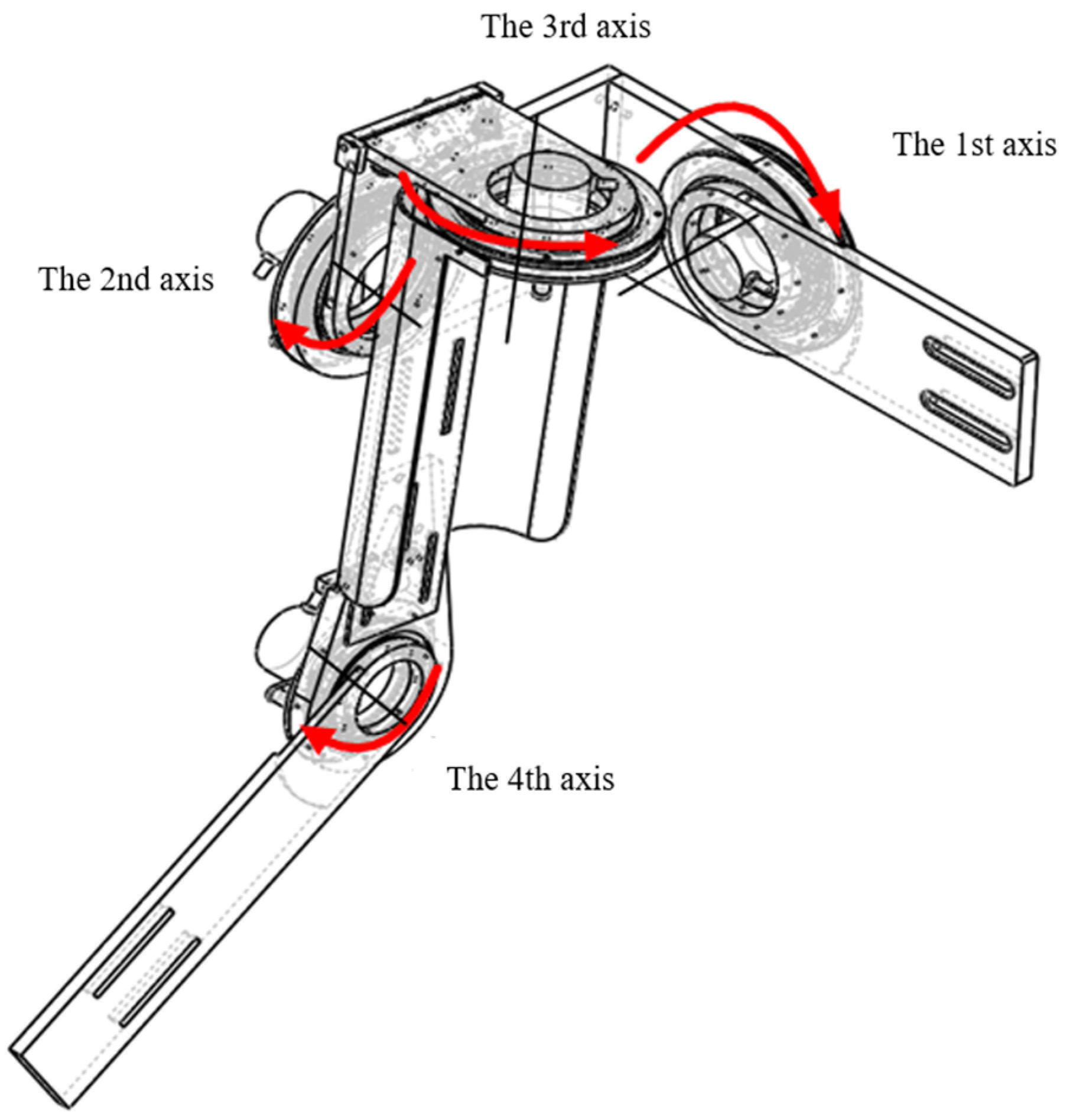
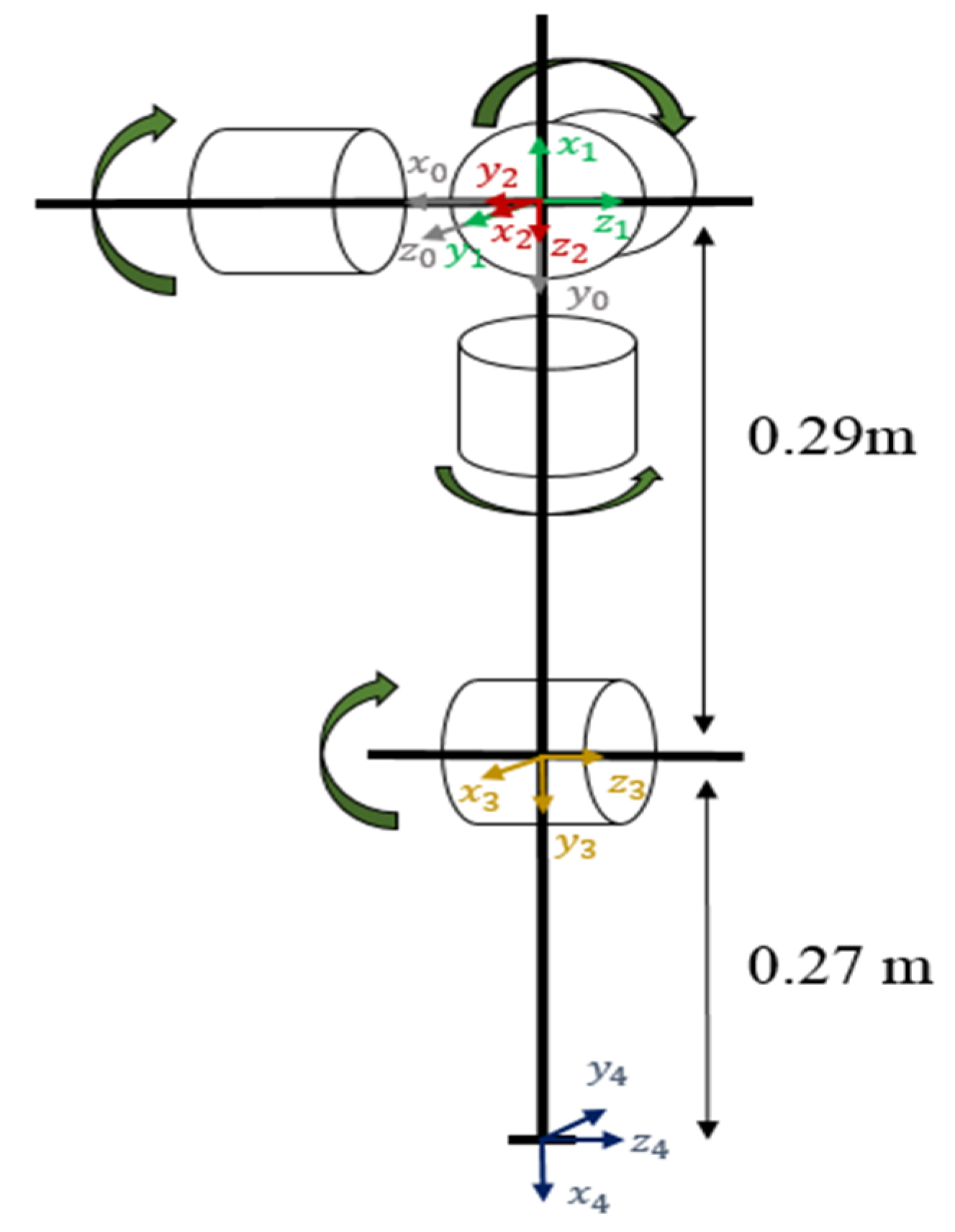
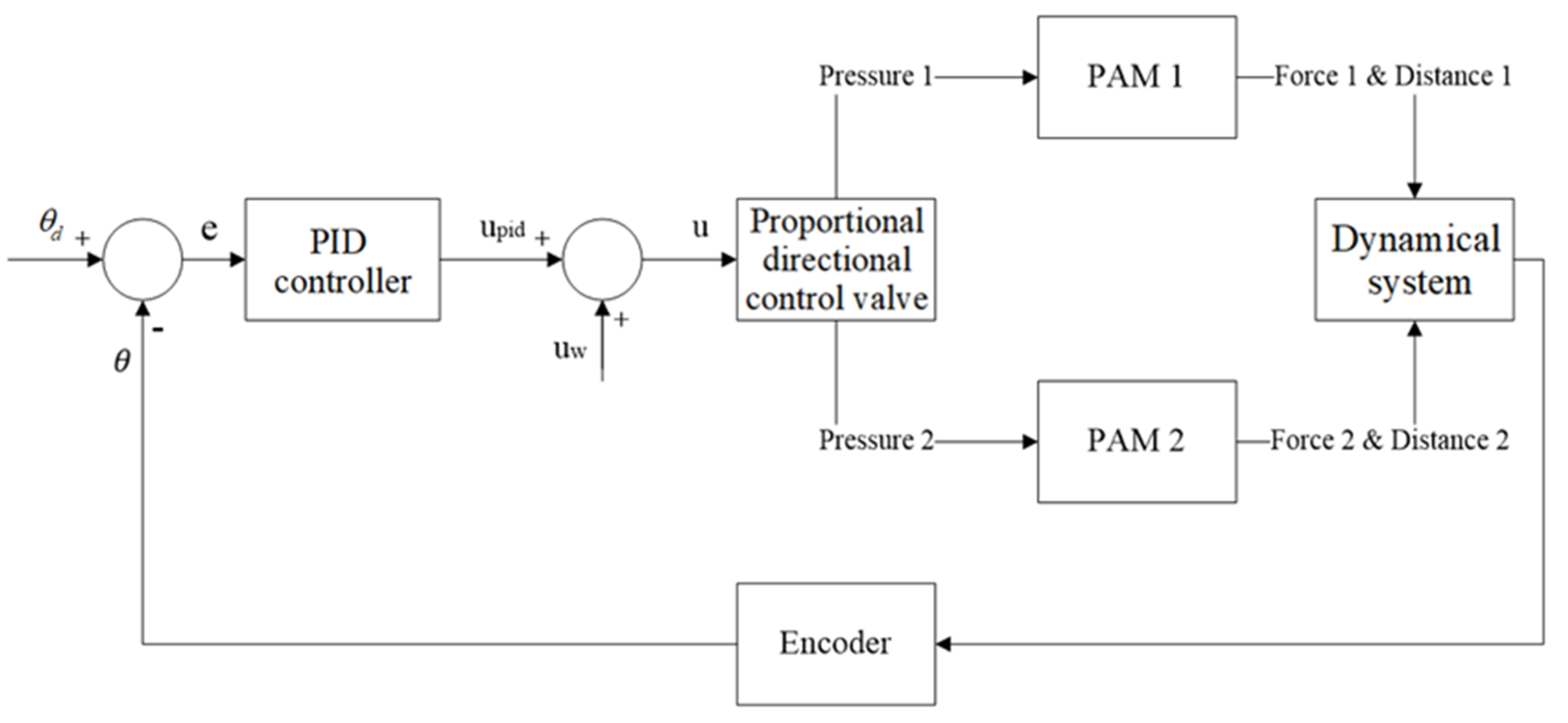
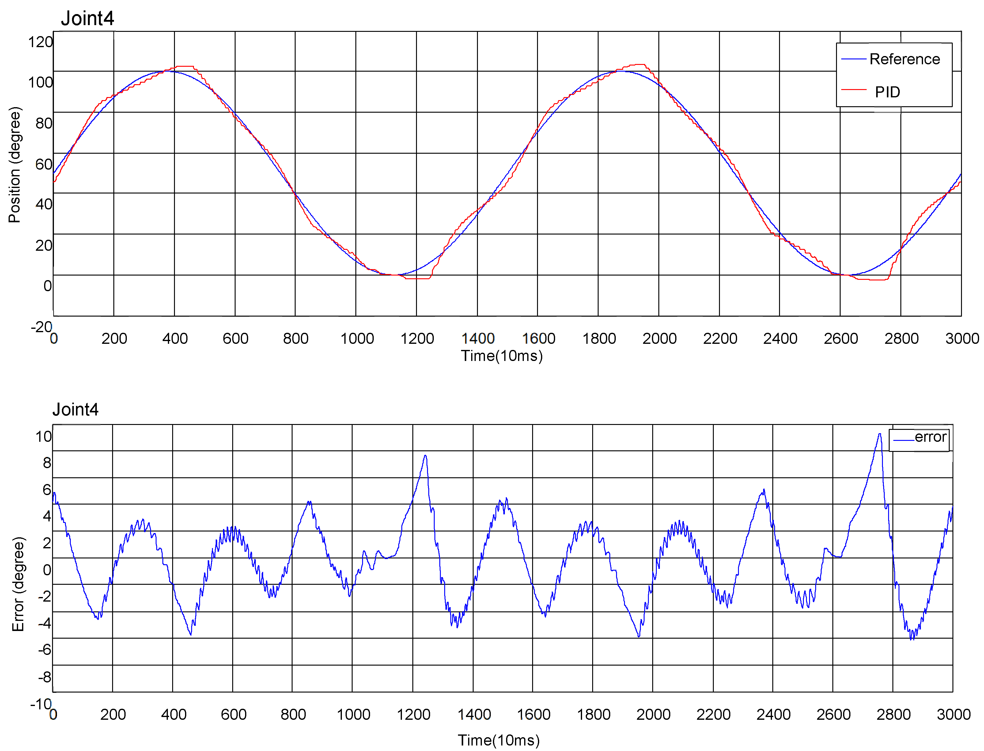
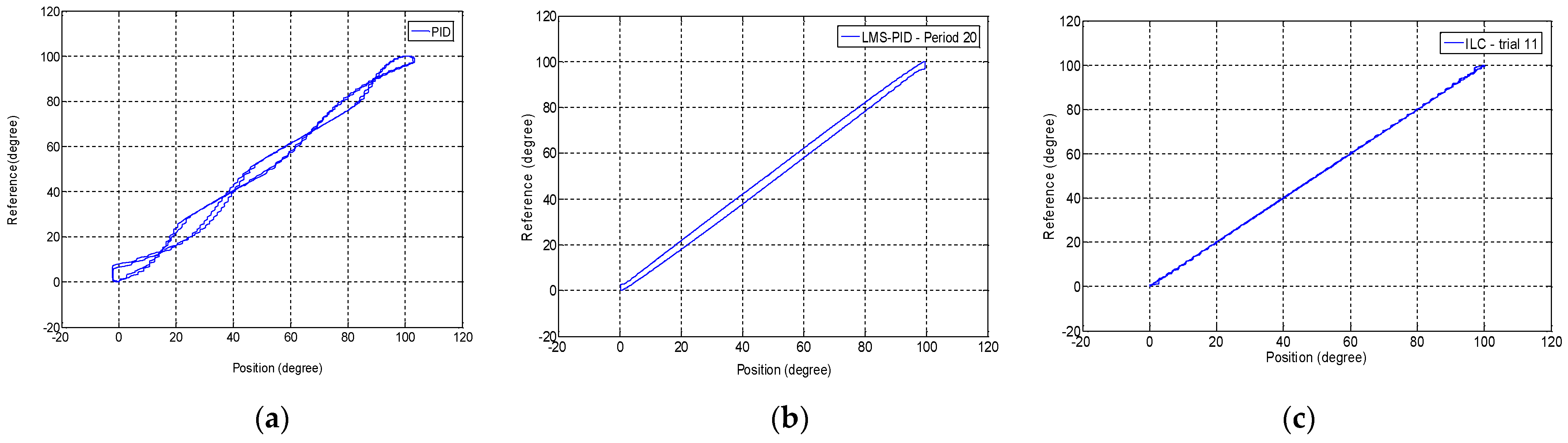
This study developed a multi-functional redundant robotic arm with four degrees of freedom using PAM as the main actuator to allow patients with upper limb mobility impairment to perform rehabilitation trajectory tasks in the future while wearing the robotic arm. The exoskeleton robot arm is designed based on the structure of the joints of the human arm due to the need to wear it on the human body. Since the mechanism may collide with the user when it is in motion, an actuator and control commands are used to limit the space available for each rotary axis during the movement of the robot arm so as not to exceed the limit of human arm joints. The rotary axis control part is controlled by PAM. Therefore, the mathematical model of the single-axis robot arm driven by two PAMs was firstly developed, followed by the design of the PID, feedback (LMS-PID), and feed-forward (ILC) controllers. Because of the complexity of the nonlinear characteristics of the PAM actuator, the model and control parameters are uncertain when performing the tracking experiment of the PID controller by simulating the parameters, which leads to the ineffective control of the parameters.

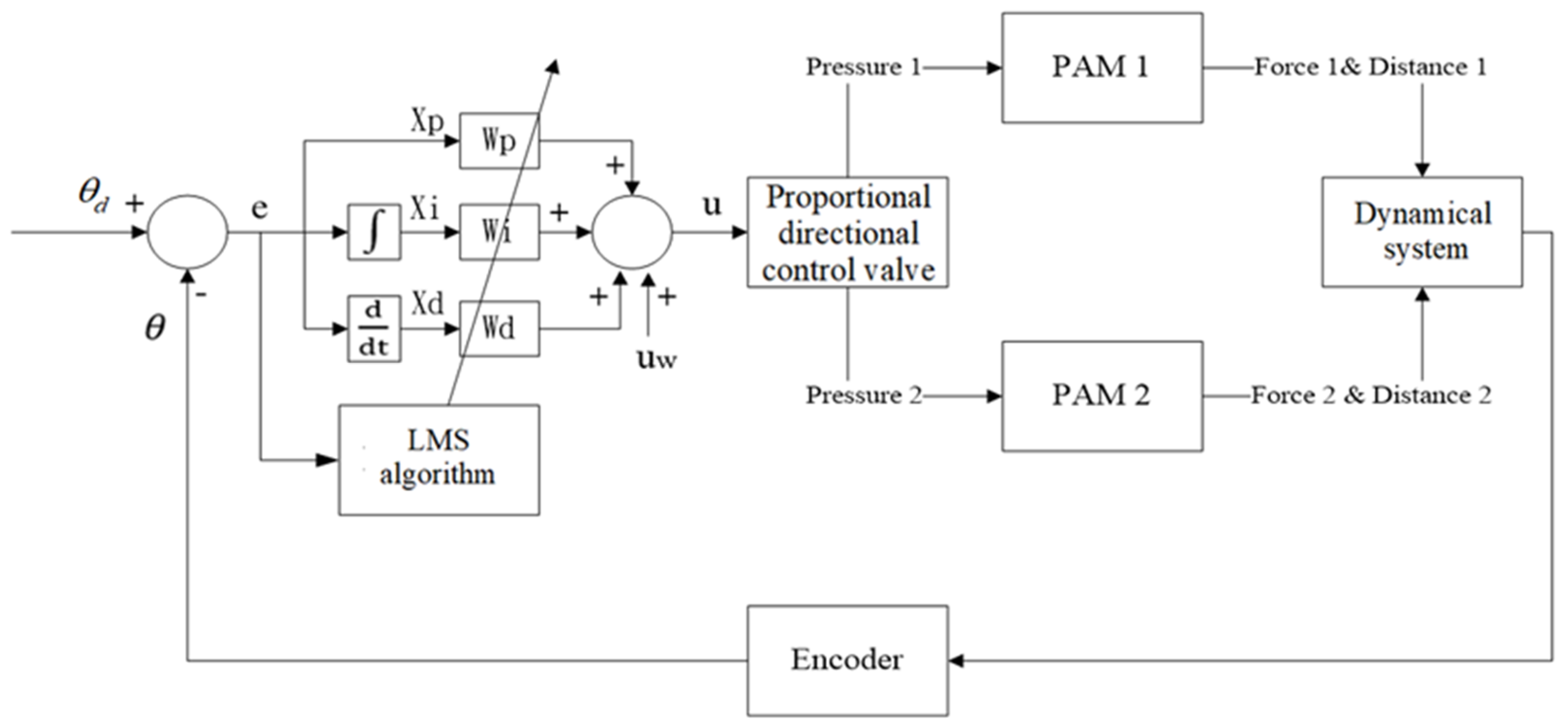
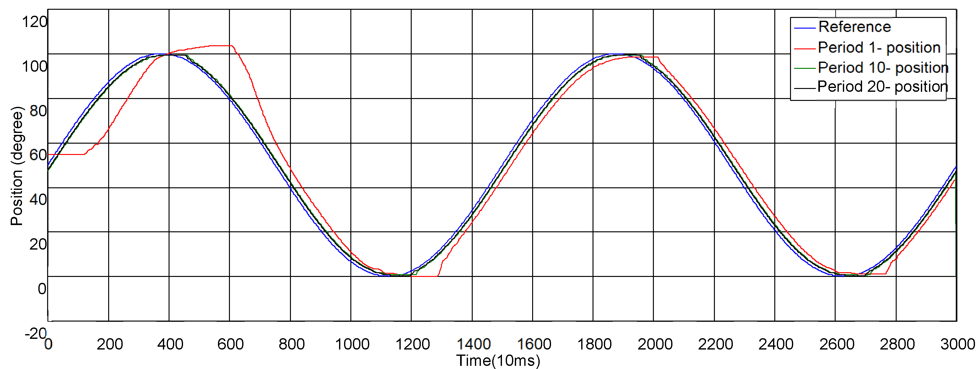
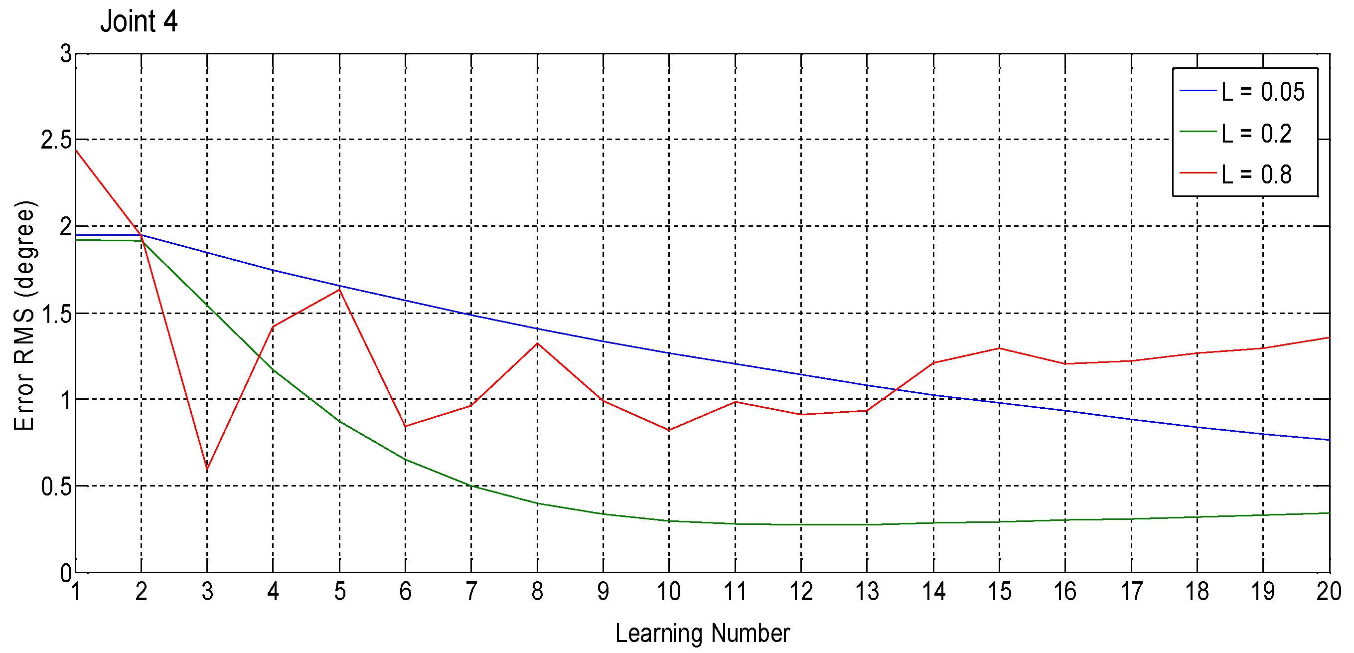
Therefore, this study used a self-adaptive (LMS-PID) controller and an iterative learning controller (ILC) to compensate; the ILC performs the feed-forward compensation by iteratively modifying the control commands, while the LMS-PID controller is an adaptive feedback controller using the LMS algorithm. The parameters obtained from the LMS-PID combined with the iterative learning control can produce a better control effect, especially the phase lag and transient parts, which cannot be solved by the PID controller. Iterative learning control can reduce the error of the system to a certain range within a limited number of learning times, which can greatly improve the control effect of the robot arm.

Overall, in the single-axis robotic arm controller experiment, the results showed that LMS-PID was superior to the conventional PID control method. In the control experiment of the robotic arm under multi-axis recovery trajectory, the experimental results showed that the study can plan the training of drawing a circle on the wall, which can effectively train the shoulder joint area. In the multi-axis robotic tracking experiment under the rehabilitation trajectory, the results showed that the LMS-PID controller reduced the RMSE of the tracking trajectory to 0.2444 and 0.2853. In the robotic arm joining/loading experiment, the results showed that the tracking accuracy was still accurate after the loading.

Finally, the robotic arm in the rehabilitation mode was only used by people without impairments, but the purpose of this development is for patients with arm injuries. It is hoped that we can cooperate with hospitals in the future so that patients with arm disabilities can use the robotic arm developed by this study to perform rehabilitation exercises.

References

1. Smith, R.; Cucco, E.; Fairbairn, C. Robotic Development for the Nuclear Environment: Challenges and Strategy. Robotics 2020, 9, 94. [Google Scholar] [CrossRef]
2. Rojas, R.A.; Wehrle, E.; Vidoni, R. A Multicriteria Motion Planning Approach for Combining Smoothness and Speed in Collaborative Assembly Systems. Appl. Sci. 2020, 10, 5086. [Google Scholar] [CrossRef]
3. Atmoko, R.A.; Yang, D.; Adhitya, R.Y. Cloud Robotics Architecture and Challenges on Disaster Mangement. AIP Conf. Proc. 2020, 2278, 020033. [Google Scholar]
4. Bai, S.; Christensen, S.; Islam, M.R.U. An upper-body exoskeleton with a novel shoulder mechanism for assistive applications. In Proceedings of the 2017 IEEE International Conference on Advanced Intelligent Mechatronics, Munich, Germany, 3–7 July 2017; pp. 1041–1046. [Google Scholar]
5. Castro, M.N.; Rasmussen, J.; Andersen, M.S.; Bai, S. A compact 3-DOF shouder mechanism constructed with scissors linkages for exoskeleton applications. Mech. Mach. Theroy 2019, 132, 264–278. [Google Scholar] [CrossRef]
6. Armotion. Available online: https://www.neurorehabdirectory.com/rehab-products/armotion/ (accessed on 18 July 2022).
7. Nakaoka, S.; Nakazawa, A.; Kanehiro, F.; Ikeuchi, K. Learning from Observation Paradigm: Leg Task Models for Enabling a Biped Humanoid Robot to Imitate Human Dances. Int. J. Robot. Res. 2007, 26, 829–844. [Google Scholar] [CrossRef]
8. Truelsen, T.; Bonita, R. The worldwide burden of stroke: Current status and future projections. Handb. Clin. Neurol. 2008, 92, 327–336. [Google Scholar]
9. Ulrich, K.; Eppinger, S. EBOOK: Product Design and Development; McGraw Hill: New York, NY, USA, 2011. [Google Scholar]
10. Gull, M.A.; Bai, S.; Bak, T. A Review on Design of Upper Limb Exoskeletons. Robotics 2020, 9, 16. [Google Scholar] [CrossRef]
11. Schulte, H. The Characteristics of the McKibben artifical muscle. In The Application of External Power in Prosthetcis and Orthotics; National Academy of Sciences-National Research Council: Washington, DC, USA, 1961; pp. 94–115. [Google Scholar]
12. Liu, J.; Zuo, S.; Wang, L.; Zhang, Y. Simulation Investigation of a Soft Hydraulic Artificial Muscle. Journal of Physics: Conference Series. In Proceedings of the 2021 International Conference on Mechanical Engineering, Intelligent Manufacturing and Automation Technology (MEMAT), Guilin, China, 15–17 January 2021; p. 012068. [Google Scholar]
13. Matisková, D.; Čakurda, T.; Marasová, D.; Balara, A. Determination of the Function of the Course of the Static Property of PAMs as Actuators in Industrial Robotics. Appl. Sci. 2021, 11, 7288. [Google Scholar] [CrossRef]
14. Ferraresi, C.; Muscolo, G.G.; De Benedictis, C.; Paterna, M.; Gisolo, S.M. Design and Modeling of a Novel Pneumatic Passive Upper Limb Exoskeleton Based on McKibben Artificial Muscle. 2021. Available online: https://webthesis.biblio.polito.it/19574/1/tesi.pdf (accessed on 18 July 2022).
15. Boblan, I.; Schulz, A. A humanoid muscle robot torso with biologically inspired construction. In Proceedings of the ISR 2010 (41st International Symposium on Robotics) and ROBOTIK 2010 (6th German Conference on Robotics), Munich, Germany, 7–9 June 2010; pp. 1–6. [Google Scholar]
16. Lin, C.-J. Motion planning of redundant robots by perturbation method. Mechatronics 2004, 14, 281–297. [Google Scholar] [CrossRef]
17. Tondu, B.; Ippolito, S.; Guiochet, J.; Daidie, A. A seven-degrees-of-freedom robot-arm driven by pneumatic artificial muscles for humanoid robots. Int. J. Robot. Res. 2005, 24, 257–274. [Google Scholar] [CrossRef]
18. Caldwell, D.G.; Tsagarakis, N.G.; Kousidou, S.; Costa, N.; Sarakoglou, I. “Soft” exoskeletons for upper and lower body rehabilition- design, control and testing. Int. J. Hum. Robot. 2007, 4, 549–573. [Google Scholar] [CrossRef]
19. Minh, T.V.; Tjahjowidodo, T.; Ramon, H.; Van Brussel, H. Cascade position control of a single pneumatic artificial muscle–mass system with hysteresis compensation. Mechatronics 2010, 20, 402–414. [Google Scholar] [CrossRef]
20. Shen, X. Nonlinear model-based control of pneumatic artificial muscle servo systems. Control. Eng. Pract. 2010, 18, 311–317. [Google Scholar] [CrossRef]
21. Andrikopoulos, G.; Nikolakopoulos, G.; Manesis, S. Non-linear control of pneumatic artificial muscles. In Proceedings of the 21st Mediterranean Conference on Control and Automation, Chania, Greece, 25–28 June 2013; pp. 729–734. [Google Scholar]
22. Uchiyama, M. Formation of high-speed motion pattern of a mechanical arm by trial. Trans. Soc. Instrum. Control. Eng. 1978, 14, 706–712. [Google Scholar] [CrossRef]
23. Arimoto, S.; Kawamura, S.; Miyazaki, F. Bettering operation of robots by learning. J. Robot. Syst. 1984, 1, 123–140. [Google Scholar] [CrossRef]
24. Fang, Y.; Chow, T.W. Iterative learning control of linear discrete-time multivariable systems. Automatica 1998, 34, 1459–1462. [Google Scholar] [CrossRef]
25. Amann, N.; Owens, D.H.; Rogers, E. Iterative learning control for discrete-time systems with exponential rate of convergence. IEE Proc.-Control. Theory Appl. 1996, 143, 217–224. [Google Scholar] [CrossRef]
26. Kurek, J.E.; Zaremba, M.B. Iterative learning control synthesis based on 2-D system theory. IEEE Trans. Autom. Control. 1993, 38, 121–125. [Google Scholar] [CrossRef]
27. Geng, Z.; Lee, J.D.; Carroll, R.L.; Haynes, L. Learning control system design based on 2D theory-an application to parallel link manipulator. In Proceedings of the IEEE International Conference on Robotics and Automation, Cincinnati, OH, USA, 13–18 May 1990; pp. 1510–1515. [Google Scholar]
28. Chow, T.W.; Fang, Y. An iterative learning control method for continuous-time systems based on 2-D system theory. IEEE Trans. Circuits Syst. I Fundam. Theory Appl. 1998, 45, 683–689. [Google Scholar] [CrossRef]
29. Moore, K.L. Iterative Learning Control for Deterministic Systems; Springer: Berlin/Heidelberg, Germany, 2012. [Google Scholar]
30. Reddy, A.C. Difference between Denavit-Hartenberg (DH) classical and modified conventions for forward kinematics of robots with case study. In Proceedings of the International Conference on Advanced Materials and manufacturing Technologies (AMMT), Hyderabad, India, 18–20 December 2014; pp. 267–286. [Google Scholar]
31. Jacob, N.; Kaur, B. Combining LMS with PID control for H-bridge controlled thermal electric cooler (TEC). In Proceedings of the Mobile Multimedia/Image Processing, Security, and Applications 2020, Online, 27 April–8 May 2020; p. 1139905. [Google Scholar]
32. Widrow, B.; Hoff, M.E. Adaptive Switching Circuits; Stanford Univ Ca Stanford Electronics Labs: New York, NY, USA, 1960. [Google Scholar]
33. Hunsaker, F.G.; Cioffi, D.A.; Amadio, P.C.; Wright, J.G.; Caughlin, B. The American academy of orthopaedic surgeons outcomes instruments: Normative values from the general population. JBJS 2002, 84, 208–215. [Google Scholar] [CrossRef]
34. Baysal, C.V. An Inverse Dynamics-Based Control Approach for Compliant Control of Pneumatic Artificial Muscles. Actuators 2022, 11, 111. [Google Scholar] [CrossRef]
35. Liang, D.K.; Sun, N.; Wu, Y.M.; Chen, Y.H.; Fang, Y.C.; Liu, L.Q. Energy-Based Motion Control for Pneumatic Artificial Muscle Actuated Robots With Experiments. IEEE Trans. Ind. Electron. 2022, 69, 7295–7306. [Google Scholar] [CrossRef]
36. Yang, Q.Y.; Wang, W.; Zhang, Y.T.; Yan, Q.Z.; Cai, J.P. Angle Error-Tracking Iterative Learning Control for Pneumatic Artificial Muscle System. IEEE Access 2021, 9, 163099–163107. [Google Scholar] [CrossRef]
37. Liu, X.; Zhang, J.H.; Xu, F.; Wang, T.; Zhao, L. Design and Modelling of Multi-DOF Manipulator Driven by Hysteresis-Attenuated Pneumatic Artificial Muscles. IEEE Robot. Autom. Lett. 2022, 7, 6447–6454. [Google Scholar] [CrossRef]
38. Liu, G.D.; Sun, N.; Liang, D.K.; Chen, Y.H.; Yang, T.; Fang, Y.C. Neural network-based adaptive command filtering control for pneumatic artificial muscle robots with input uncertainties. Control. Eng. Pract. 2022, 118, 104960. [Google Scholar] [CrossRef]
39. Buchler, D.; Guist, S.; Calandra, R.; Berenz, V.; Scholkopf, B.; Peters, J. Learning to Play Table Tennis From Scratch Using Muscular Robots. IEEE Trans. Robot. 2022. [Google Scholar] [CrossRef]
40. Jiang, F.L.; Liu, H.; Chai, D.X. Humanoid Lower Limb: Design, Analysis, Observer-Based Fuzzy Adaptive Control and Experiment. Math. Probl. Eng. 2021, 2021, 1–5. [Google Scholar] [CrossRef]
Figure 1. Schematic diagram of robotic arm structure.
Applsci 12 08419 g001
Figure 2. Schematic diagram of robotic arm shoulder and elbow rotating axis operation.
Applsci 12 08419 g002
Figure 3. Schematic diagram of the complete structure of the robotic arm.
Applsci 12 08419 g003
Figure 4. Schematic diagram of the relationship of the robotic arm coordinate system.
Applsci 12 08419 g004
Figure 5. Schematic diagram of the drive of robotic arm (1st axis).
Applsci 12 08419 g005
Figure 6. Schematic diagram of the drive of robotic arm (2nd, 3rd, and 4th axes).
Applsci 12 08419 g006
Figure 7. Flow chart of PID controller applied to proportional directional control valve.
Applsci 12 08419 g007
Figure 8. Flow chart of LMS-PID controller applied to proportional directional control valve.
Applsci 12 08419 g008
Figure 9. Tracking and error diagrams of PID simulation parameters applied to real system.
Applsci 12 08419 g009
Figure 10. Dual PAM pressure output of PID simulation parameters applied to real system.
Applsci 12 08419 g010
Figure 11. Sin wave-tracking experiment based on LMS-PID controller.
Applsci 12 08419 g011
Figure 12. RMSE convergence curve based on LMS-PID tracking control.
Applsci 12 08419 g012
Figure 13. RMSE convergence curves for different convergence factors in the tracking experiment.
Applsci 12 08419 g013
Figure 14. Convergence curves of RMSE with different learning rates under tracking experiment.
Applsci 12 08419 g014
Figure 15. (a) Curve of the relationship between desired trajectory and PID controller tracking results. (b) Curve of the relationship between the desired trajectory and the tracking result of LMS-PID controller. (c) Curve of the relationship between expected trajectory and ILC tracing results.
Applsci 12 08419 g015
Figure 16. Four axes—curve of position rise versus time.
Applsci 12 08419 g016
Figure 17. Four axes—curve of position drop versus time.
Applsci 12 08419 g017
Figure 18. Motion trajectory 1 of each axis of the robot arm is planned by kinematics.
Applsci 12 08419 g018
Figure 19. Motion trajectory 2 of each axis of the robot arm is planned by kinematics.
Applsci 12 08419 g019
Figure 20. Trajectory 1—four axes—LMS-PID—curve charts of the controller parameters returned by tracking the 20th cycle.
Applsci 12 08419 g020
Figure 21. Trajectory 2—four axes—LMS-PID—curve charts of the controller parameters returned by tracking the 20th cycle.
Applsci 12 08419 g021
Figure 22. Schematic diagram of the robotic arm in the loading experiment.
Applsci 12 08419 g022
Figure 23. Trajectory 1—1st-axis (load-on) ILC trial 1 and trial 12 tracking and error diagrams.
Applsci 12 08419 g023
Figure 24. Trajectory 1—2nd-axis (load-on) ILC trial 1 and trial 20 tracking and error diagrams.
Applsci 12 08419 g024
Figure 25. Trajectory 1—3rd-axis (load-on) ILC trial 1 and trial 20 tracking and error diagrams.
Applsci 12 08419 g025
Figure 26. Trajectory 1—4th-axis (load-on) ILC trial 1 and trial 15 tracking and error diagrams.
Applsci 12 08419 g026