
Breast Lesions Screening of Mammographic Images with 2D Spatial and 1D Convolutional Neural Network-Based Classifier

 ,
, 


Abstract
:1. Introduction
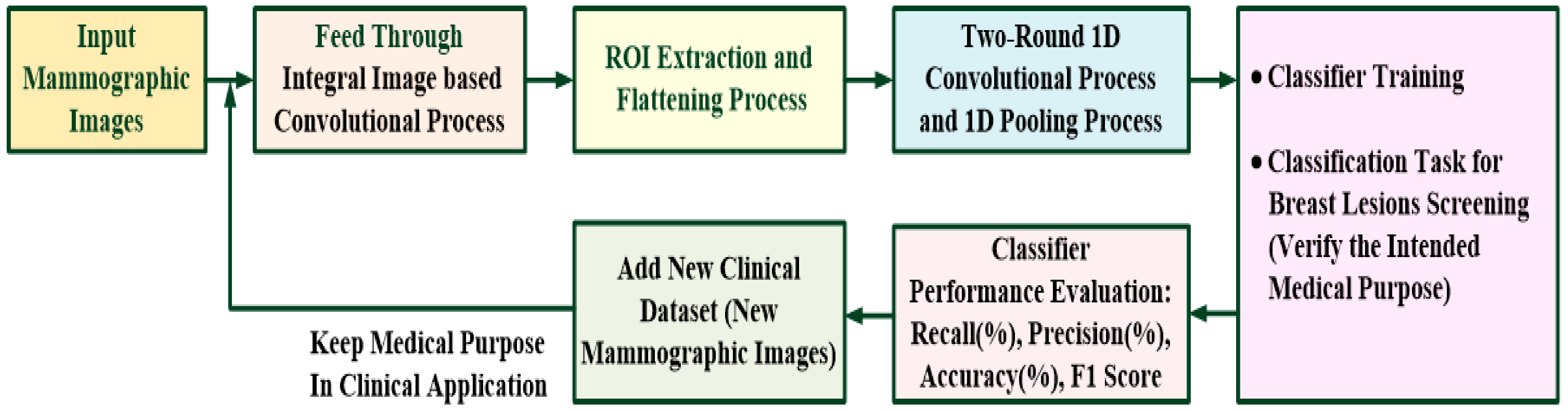
2. Methodology
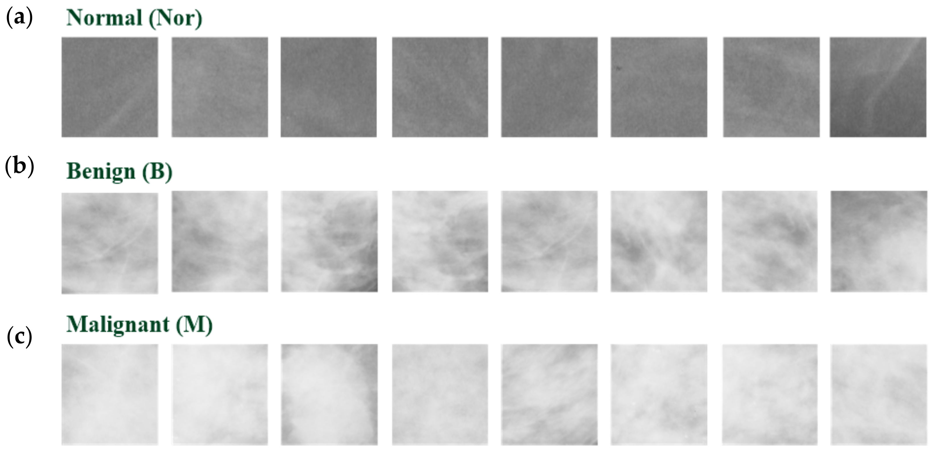
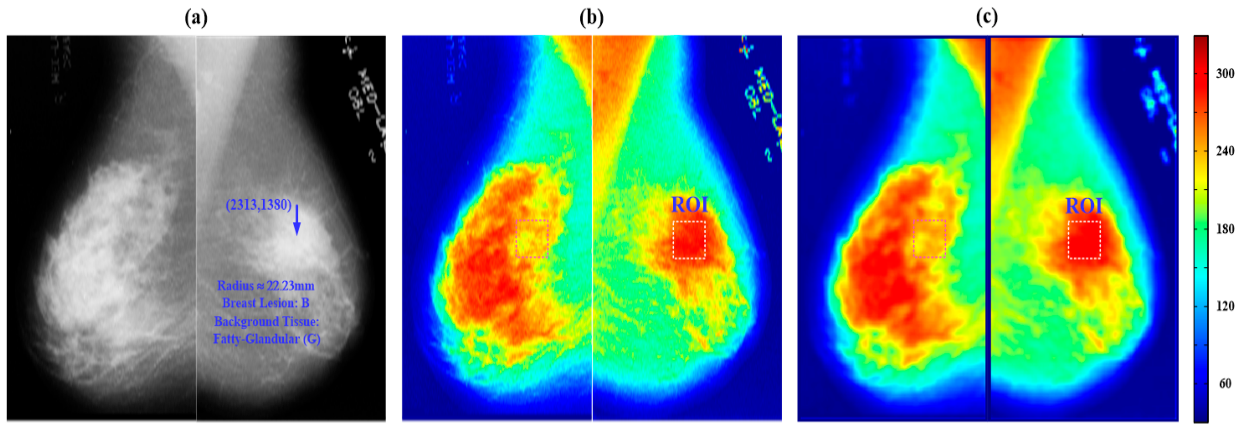
2.1. Mammographic Images Collection
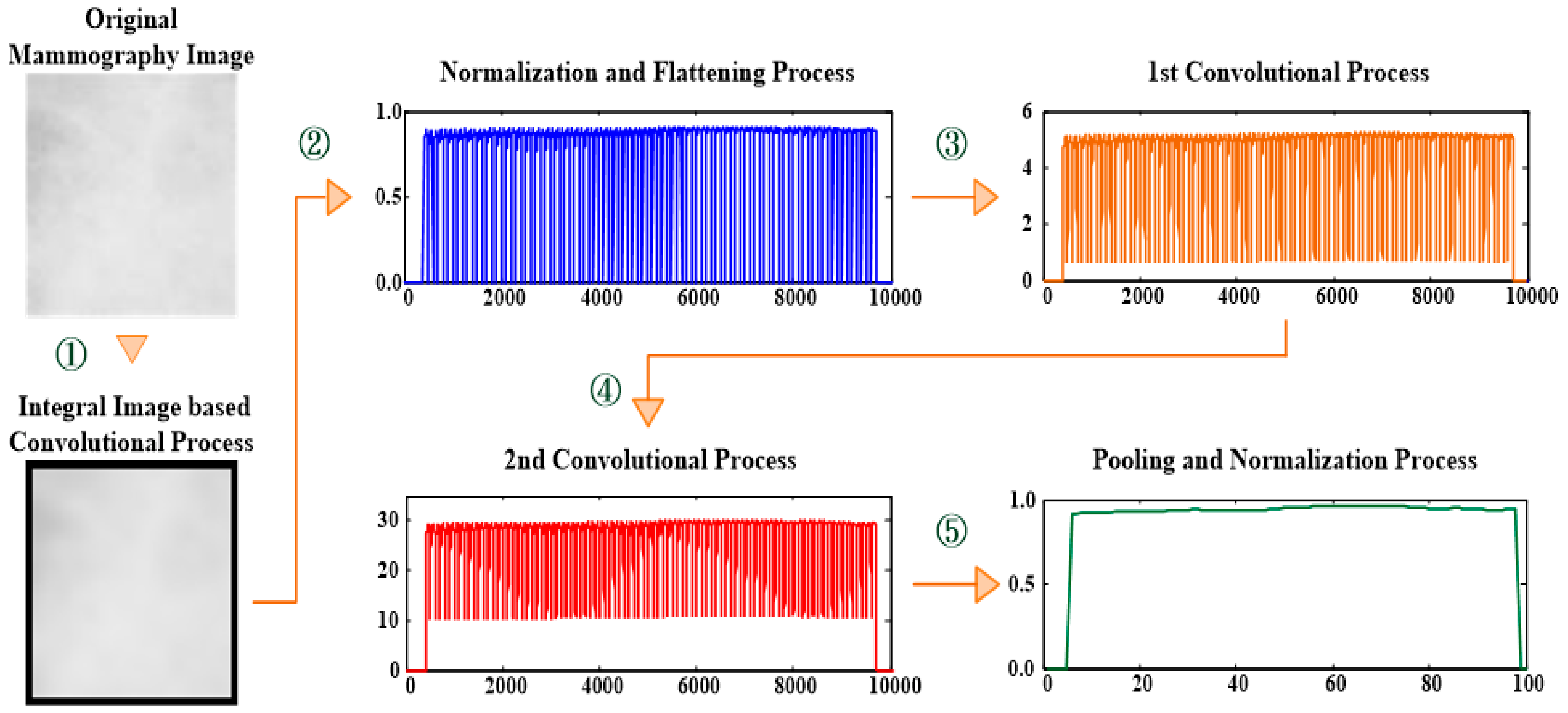
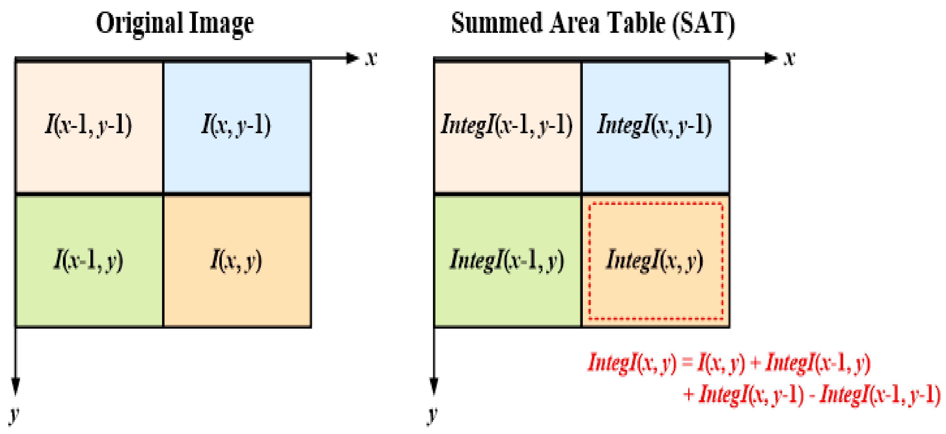
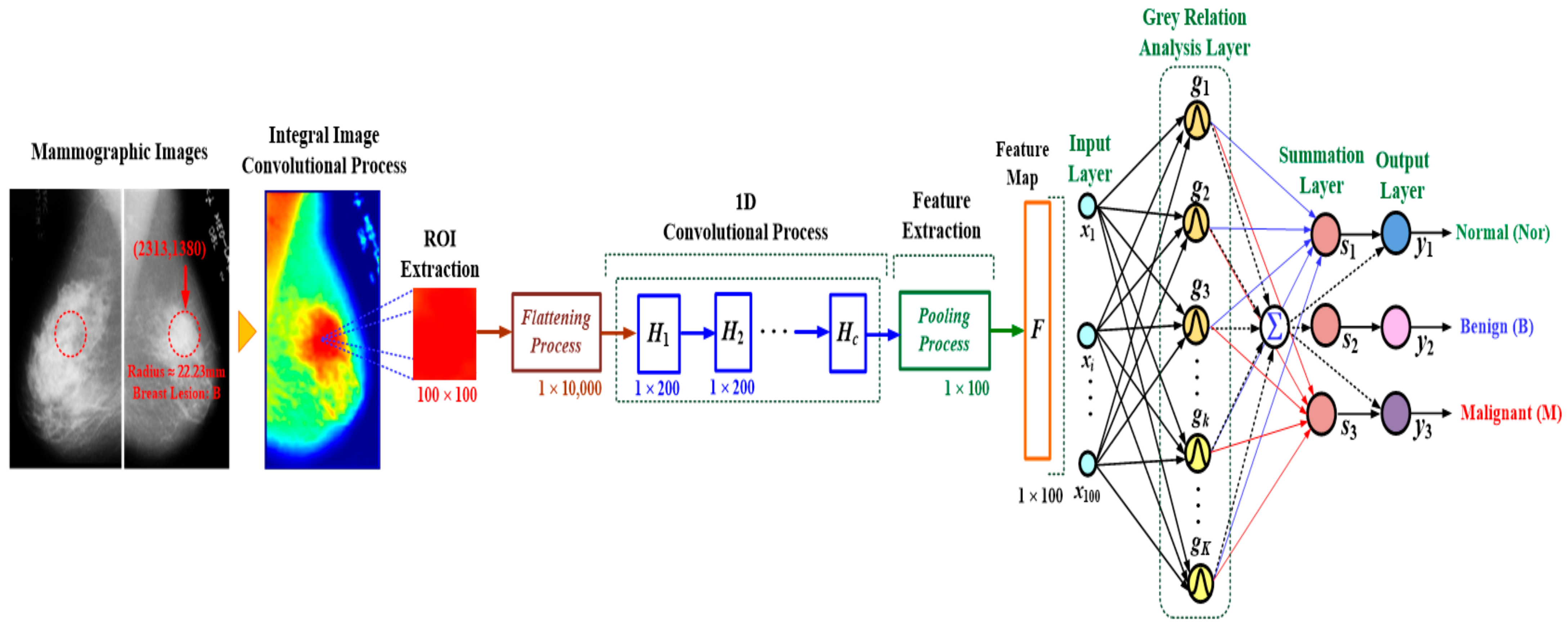
2.2. Integral Image (II)-Based Convolutional Process
2.3. Feature Extraction with Multi-Round 1D Convolutional Processes and 1D Pooling Process
2.4. Breast Lesions Screening with a GRA-Based Classifier
3. Experimental Results and Discussion
3.1. Experimental Setup
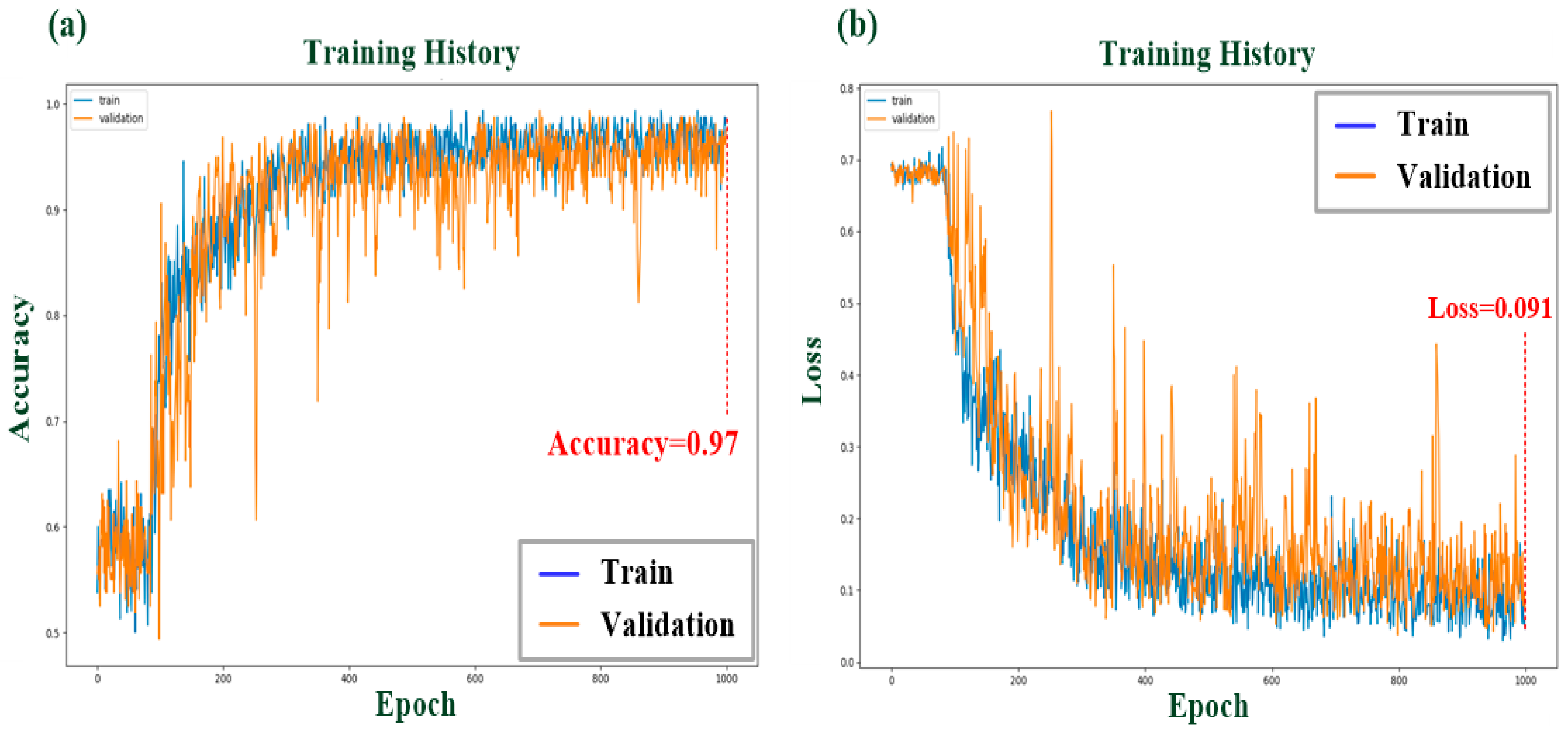
3.2. Multilayer CNN-Based Classifiers’ Training and Validation
3.3. Discussion
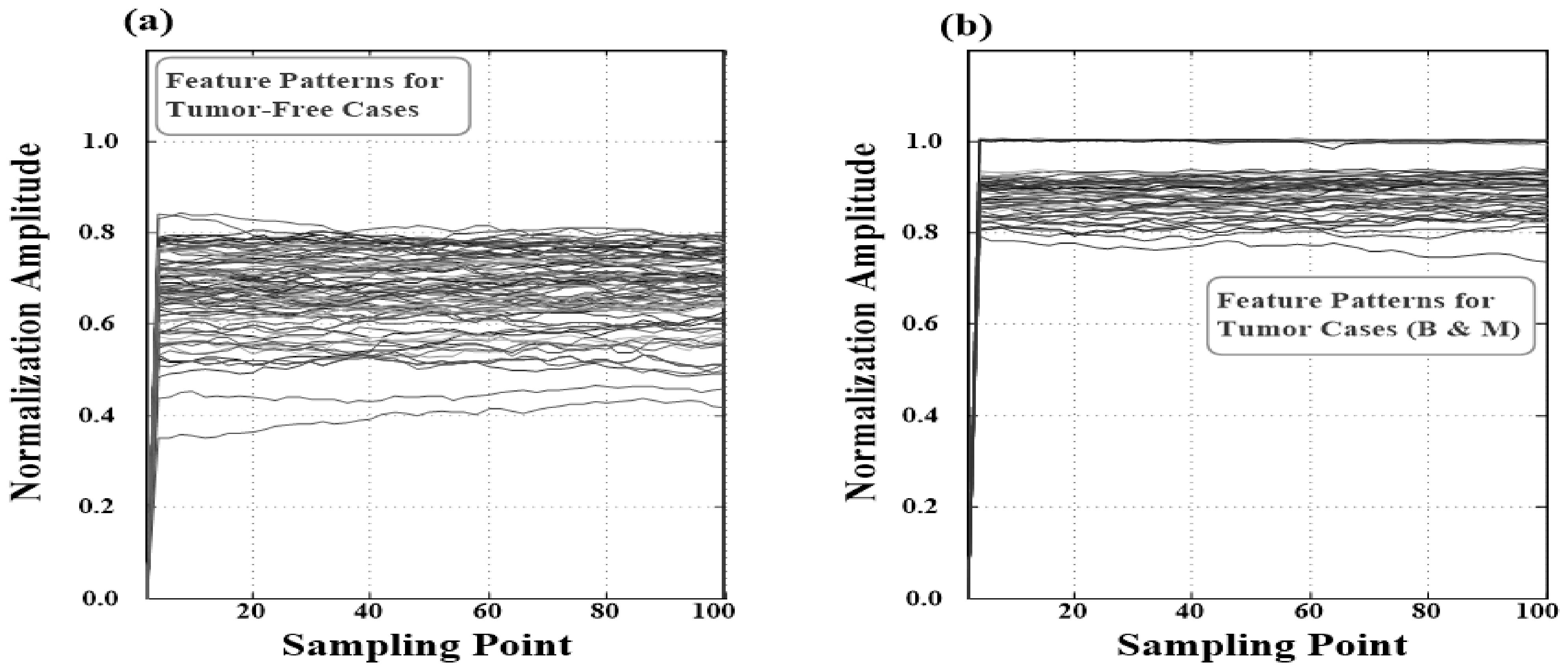
- The possible breast lesions’ spatial and edge information could be enhanced by the II-based spatial convolutional process in the first convolutional layer, which helped to easily locate ROI and extract feature patterns from the original mammographic image;
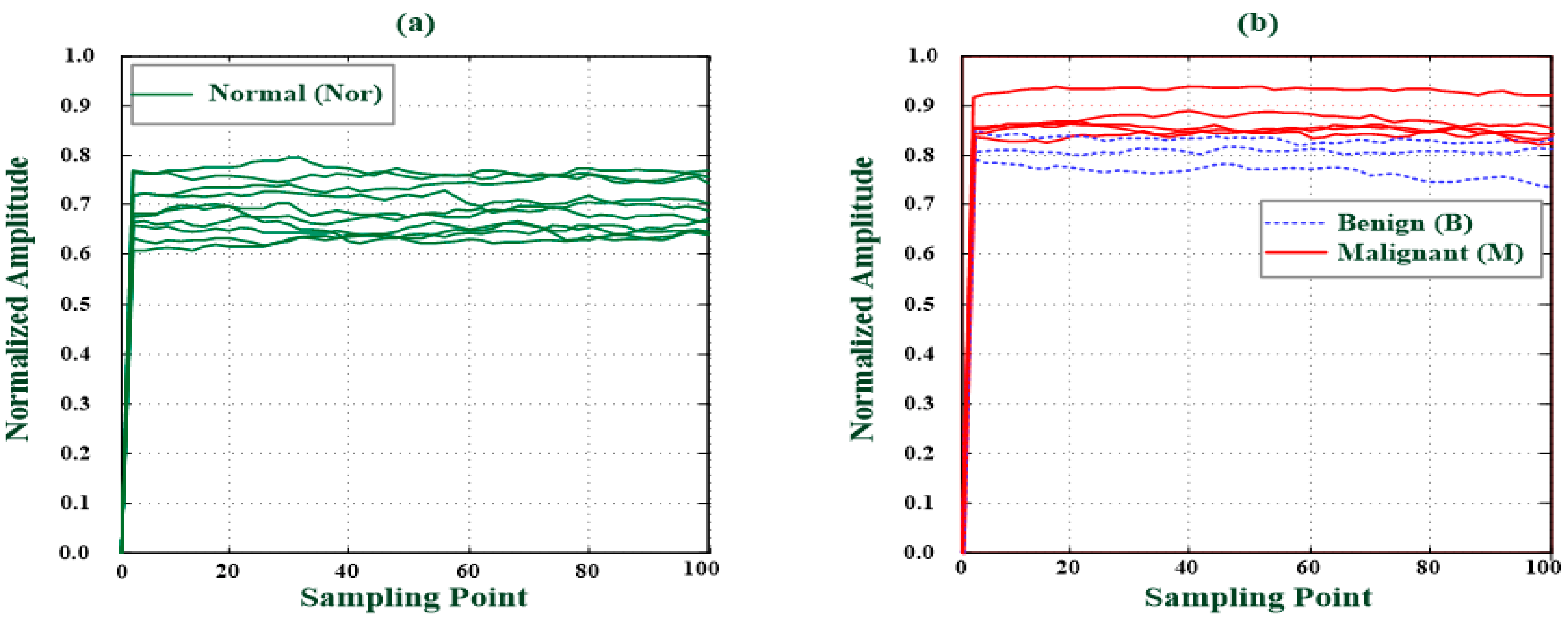
- The suitable two-round 1D convolutional processes could quantify the different levels, which helped to preliminary separate the Nor from the B and M classes;
- The dimension of feature signals could be reduced by the 1D pooling process, which helped to overcome the classifier’s overfitting problems in the training stage;
- The straightforward mathematic operations performed the training and pattern recognition tasks;
- The optimal parameters that were updated in the training stage did not require convergence condition assignment and parameters adjustment;
- The determination network parameters did not require complex iteration computations and optimization algorithms.
- The classification accuracy could be obtained in less computation time and was feasible to replace manual screening with specific expertise and experience.
4. Conclusions
Author Contributions
Funding
Institutional Review Board Statement
Informed Consent Statement
Data Availability Statement
Conflicts of Interest
Abbreviations
| CNN | Convolutional Neural Network |
| 2D | Two-Dimensional |
| 1D | One-Dimensional |
| ROI | Region of Interest |
| Nor | Normal |
| B | Benign |
| M | Malignant |
| GRA | Gray Relational Analysis |
| AI | Artificial Intelligence |
| ML | Machine Learning |
| DL | Deep Learning |
| MRI | Magnetic Resonance Imaging |
| CT | Computed Tomography |
| BI-RADS | Breast Imaging-Reporting and Data System |
| DDSM | Digital Database of Screening Mammography |
| MIAS | Mammographic Image Analysis Society |
| SVM | Support Vector Machine |
| ANN | Artificial Neural Network |
| FCN | Fully Convolutional Network |
| R-CNN | Region-based CNN |
| TTCNN | Transferable Texture Convolutional Neural Network |
| Grad-CAM | Gradient-Weighted Class Activation Mapping |
| GAP | Global Average Pooling |
| DNN | Deep Neural Network |
| CM | Clustering Method |
| II | Integral Image |
| SAT | Summed Area Table |
| MP | Maximum Pooling |
| BPNN | Back-Propagation Neural Network |
| ADAM | Adaptive Moment Estimation Method |
| GPU | Graphics Processing Unit |
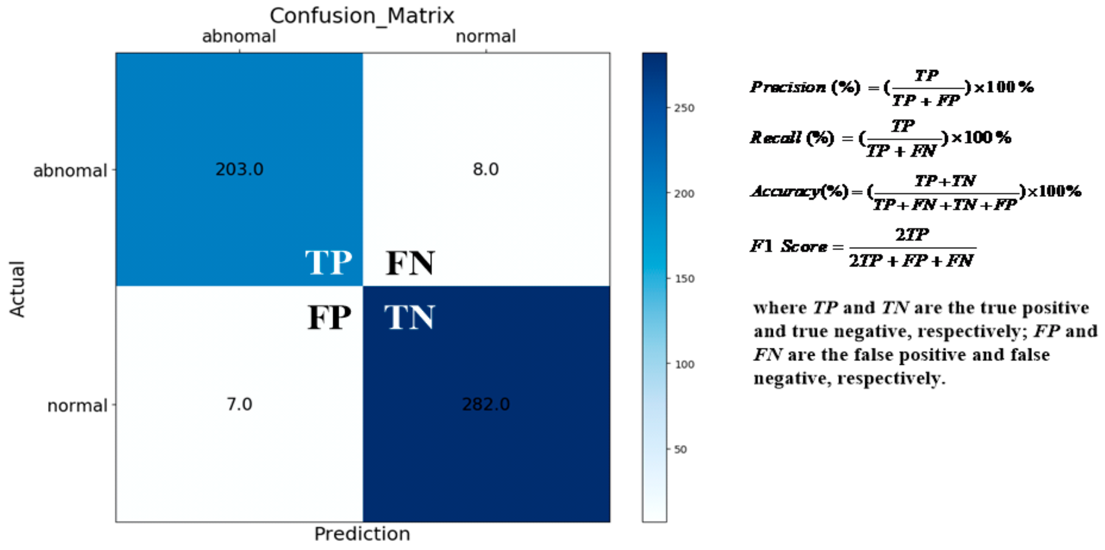
| TP | True Positive |
| FP | False Positive |
| TN | True Negative |
| FN | False Negative |
| PPV | Positive Predictive Value |
| SaMD | Software in a Medical Device |
References
- World Cancer Day 2021: Spotlight on IARC Research Related to Breast Cancer. 1965–2022. Available online: https://www.iarc.who.int/featured-news/world-cancer-day-2021/ (accessed on 24 July 2022).
- Ministry Health and Welfare, Taiwan. 2021. Cause of Death Statistics, 2022 Years. Available online: https://dep.mohw.gov.tw/dos/lp-1800-113.html (accessed on 24 July 2022).
- Liu, Q.; Liu, Z.; Yong, S.; Jia, K.; Razmjooy, N. Computer-aided breast cancer diagnosis based on image segmentation and interval analysis. Automatika 2020, 61, 496–506. [Google Scholar] [CrossRef]
- Yassin, N.I.; Omran, S.; el Houby, E.M.; Allam, E.M. Machine learning techniques for breast cancer computer aided diagnosis using different image modalities: A systematic review. Comput. Methods Programs Biomed. 2018, 156, 25–45. [Google Scholar] [CrossRef] [PubMed]
- Hamidinekoo, A.; Denton, E.; Rampun, A.; Honnor, K.; Zwiggelaar, R. Deep learning in mammography and breast histology, an overview and future trends. Med. Image Anal. 2018, 47, 45–67. [Google Scholar] [CrossRef] [PubMed] [Green Version]
- Oza, P.; Sharma, P.; Patel, S.; Bruno, A. A bottom-up review of image analysis methods for suspicious region detection in mammograms. J. Imaging 2021, 7, 190. [Google Scholar] [CrossRef] [PubMed]
- Surendiran, B.; Vadivel, A. Mammogram mass classification using various geometric shape and margin features for early detection of breast cancer. Int. J. Med. Eng. Inform. 2021, 4, 36–54. [Google Scholar] [CrossRef]
- Mammography-Breast Imaging Lexicon. Available online: https://radiologyassistant.nl/breast/bi-rads/bi-rads-formammography-and-ultrasound-2013#mammography-breast-imaging-lexicon (accessed on 30 September 2010).
- Gemignani, M.L. Breast diseases. In Clinical Gynecologic Oncology; Elsevier: Amsterdam, The Netherlands, 2012; pp. 369–403. [Google Scholar]
- Yerakly, F.; Tadele, A.K. Histopathologic patterns of breast lesions in Hawassa university comprehensive specialized hospital, Sidama Region, Ethiopia: A six-year retrospective study. Clin. Oncol. 2022, 7, 1–9. [Google Scholar]
- Kamal, R.M.; Helal, M.H.; Mansour, S.M.; Haggag, M.A.; Nada, O.M.; Farahat, I.G.; Alieldin, N.H. Can we apply the MRI BI-RADSlexicon morphology descriptors on contrast-enhanced spectral mammography? Br. J. Radiol. 2016, 89, 1064. [Google Scholar] [CrossRef] [Green Version]
- Wedegärtner, U.; Bick, U.; Wörtler, K.; Rummeny, E.; Bongartz, G. Differentiation between benign and malignant findings on MR-mammography: Usefulness of morphological criteria. Eur. Radiol. 2001, 11, 1645–1650. [Google Scholar] [CrossRef]
- Fernandes, S.L.; Rajinikanth, V.; Kadry, S. A hybrid framework to evaluate breast abnormality using infrared thermal images. IEEE Consum. Electron. Mag. 2019, 8, 31–36. [Google Scholar] [CrossRef]
- Rajinikanth, V.; Satapathy, S.C. Segmentation of ischemic stroke lesion in brain MRI based on social group optimization and fuzzy-Tsallis entropy. Arab. J. Sci. Eng. 2018, 43, 4365–4378. [Google Scholar] [CrossRef]
- Morris, E.A.; Comstock, C.E.; Lee, C.H. ACR BIRADS® magnetic resonance imaging. In ACR BI-RADS® Atlas, Breast Imaging Reporting and Data System; American College of Radiology: Reston, VA, USA, 2013. [Google Scholar]
- Sickles, E.; d’Orsi, C.; Bassett, L.; Appleton, C.; Berg, W.; Burnside, E.; Feig, S.; Gavenonis, S.; Newell, M.; Trinh, M. Acr bi-rads® mammogramphy. In ACR BI-RADS® Atlas Breast Imaging Reporting and Data System; American College of Radiology: Reston, VA, USA, 2013; Volume 5. [Google Scholar]
- Breast Imaging-Reporting and Data System (BI-RADS). Available online: https://radiopaedia.org/articles/breast-imaging-reporting-and-data-system-bi-rads?lang=us (accessed on 20 July 2021).
- Bruno, A.; Ardizzone, E.; Vitabile, S.; Midiri, M. A novel solution based on scale invariant feature transform descriptors and deep learning for the detection of suspicious regions in mammogram images. J. Med. Signals Sens. 2020, 10, 158–173. [Google Scholar]
- Heath, M.; Bowyer, K.; Kopans, D.; Kegelmeyer, P.; Moore, R.; Chang, K.; Munishkumaran, S. Current status of the digital database for screening mammography. In Digital Mammography; Springer: Dordrecht, The Netherlands, 1998; pp. 457–460. [Google Scholar]
- Lee, R.S.; Gimenez, F.; Hoogi, A.; Miyake, K.K.; Gorovoy, M.; Rubin, D.L. A curated mammography data set for use in computer-aided detection and diagnosis research. Sci. Data 2017, 4, 170177. [Google Scholar] [CrossRef]
- Oliveira, J.E.; Gueld, M.O.; Araújo, A.d.A.; Ott, B.; Deserno, T.M. Toward a standard reference database for computer-aided mammography. In Medical Imaging 2008: Computer-Aided Diagnosis; International Society for Optics and Photonics: Bellingham, WA, USA, 2008; Volume 6915, p. 69151Y. [Google Scholar]
- Pilot European Image Processing Archive. The Mini-MIAS Database of Mammograms. 2012. Available online: http://peipa.essex.ac.uk/pix/mias/ (accessed on 24 July 2022).
- Mammographic Image Analysis Society. (MIAS) Database v1.21. 2019. Available online: https://www.repository.cam.ac.uk/handle/1810/250394 (accessed on 24 July 2022).
- Vijayarajeswari, R.; Parthasarathy, P.; Vivekanandan, S.; Basha, A.A. Classification of mammogram for early detection of breast cancer using SVM classifier and Hough transform. Measurement 2019, 146, 800–805. [Google Scholar] [CrossRef]
- Mahersia, H.; Boulehmi, H.; Hamrouni, K. Development of intelligent systems based on Bayesian regularization network and neuro-fuzzy models for mass detection in mammograms: A comparative analysis. Comput. Methods Programs Biomed. 2016, 126, 46–62. [Google Scholar] [CrossRef]
- Lee, J.; Nishikawa, R.M. Automated mammographic breast density estimation using a fully convolutional network. Med. Phys. 2018, 45, 1178–1190. [Google Scholar] [CrossRef]
- Kamil, M.Y.; Salih, A.M. Mammography images segmentation via Fuzzy C-mean and K-mean. Int. J. Intell. Eng. Syst. 2019, 12, 22–29. [Google Scholar] [CrossRef]
- Li, S.; Dong, M.; Du, G.; Mu, X. Attention dense-u-net for automatic breast mass segmentation in digital mammogram. IEEE Access 2019, 7, 59037–59047. [Google Scholar] [CrossRef]
- AlGhamdi, M.; Abdel-Mottaleb, M.; Collado-Mesa, F. Du-net: Convolutional network for the detection of arterial calcifications in mammograms. IEEE Trans. Med. Imaging 2020, 39, 3240–3249. [Google Scholar] [CrossRef]
- Sarker, I.H. Machine learning: Algorithms, real-world applications and research directions. SN Comput. Sci. 2021, 2, 160. [Google Scholar] [CrossRef]
- Shelhamer, E.; Long, J.; Darrell, T. Fully convolutional networks for semantic segmentation. IEEE Trans. Pattern Anal. Mach. Intell. 2017, 39, 640–651. [Google Scholar] [CrossRef]
- Xu, S.; Adeli, E.; Cheng, J.Z.; Xiang, L.; Li, Y.; Lee, S.W.; Shen, D. Mammographic mass segmentation using multichannel and multiscale fully convolutional networks. Int. J. Imaging Syst. Technol. 2020, 30, 1095–1107. [Google Scholar] [CrossRef]
- Sathyan, A.; Martis, D.; Cohen, K. Mass and calcification detection from digital mammogramsusing UNets. In Proceedings of the 2020 7th IEEE International Conference on Soft Computing & Machine Intelligence (ISCMI), Stockholm, Sweden, 14–15 November 2020; pp. 229–232. [Google Scholar]
- Agarwal, R.; Díaz, O.; Yap, M.H.; Lladó, X.; Martí, R. Deep learning for mass detection in full field digital mammograms. Comput. Biol. Med. 2020, 121, 103774. [Google Scholar] [CrossRef]
- Ben-Ari, R.; Akselrod-Ballin, A.; Karlinsky, L.; Hashoul, S. Domain specific convolutional neural nets for detection of architectural distortion in mammograms. In Proceedings of the 2017 IEEE 14th International Symposium on Biomedical Imaging, Melbourne, Australia, 18–21 April 2017; pp. 552–556. [Google Scholar]
- Zhang, Z.; Wang, Y.; Zhang, J.; Mu, X. Comparison of multiple feature extractors on Faster RCNN for breast tumor detection. In Proceedings of the 2019 8th IEEE International Symposium on Next Generation Electronics, Zhengzhou, China, 9–10 October 2019; pp. 1–4. [Google Scholar]
- Maqsood, S.; Damaševičius, R.; Maskeliunas, R. TTCNN: A breast cancer detection and classification towards computer-aided diagnosis using digital mammography in early stages. Appl. Sci. 2022, 12, 3273. [Google Scholar] [CrossRef]
- Suh, Y.J.; Jung, J.; Cho, B.-J. Automated breast cancer detection in digital mammograms of various densities via deep learning. J. Presonalized Med. 2020, 10, 211. [Google Scholar] [CrossRef]
- Chen, P.-Y.; Sun, Z.-L.; Wu, J.-X.; Pai, C.C.; Li, C.-M.; Lin, C.-H.; Pai, N.-S. Photoplethysmo graphy analysis with Duffing–Holmes self-synchronization dynamic errors and 1D CNN-based classifier for upper extremity vascular disease screening. Processes 2021, 9, 2093. [Google Scholar] [CrossRef]
- Lin, C.-H.; Zhang, F.-Z.; Wu, J.-X.; Pai, N.-S.; Chen, P.Y.; Pai, C.-C.; Kan, C.-D. Posteroanterior chest X-ray image classification with a multilayer 1D convolutional neural network based classifier for cardiomegalylevel screening. Electronics 2022, 11, 1364. [Google Scholar] [CrossRef]
- Chen, P.Y.; Zhang, X.-H.; Wu, J.-X.; Pai, C.C.; Hsu, J.-C.; Lin, C.-H.; Pai, N.-S. Automaticbreast tumor screening of mammographic images with optimal convolutional neural network. Appl. Sci. 2022, 12, 4079. [Google Scholar] [CrossRef]
- Selvaraju, R.R.; Cogswell, M.; Das, A.; Vedantam, R.; Parikh, D.; Batra, D. Grad-CAM: Visual explanations from deep networks via gradient-based localization. arXiv 2016, arXiv:1610.02391. [Google Scholar]
- Viola, P.; Jones, M. Rapid object detection using a boosted cascade of simple features. In Proceedings of the 2001 IEEE Computer Society Conference on Computer Vision and Pattern Recognition, Kauai, HI, USA, 8–14 December 2001. [Google Scholar]
- Ehsan, S.; Clark, A.F.; ur Rehman, N.; McDonald-Maier, K.D. Integral images: Efficient algorithms for their Computation and storage in resource-constrained embedded vision systems. Sensors 2015, 15, 6804. [Google Scholar] [CrossRef] [Green Version]
- Kasagi, A.; Tabaru, T.; Tamura, H. Fast algorithm using summed area tables with unified layer performing convolution and average pooling. In Proceedings of the 2017 IEEE International Workshop on Machine Learning for Signal Processing, Tokyo, Japan, 25–28 September 2017. [Google Scholar]
- Pu, Y.-F.; Zhou, J.-L.; Yuan, X. Fractional differential mask: A fractional differential-based approach for multiscale texture enhancement. IEEE Trans. Image Process. 2010, 19, 491–511. [Google Scholar]
- Zhang, Y.; Pu, Y.-F.; Zhou, J.-L. Construction of fractional differential masks based on Riemann-Liouville definition. J. Comput. Inf. Syst. 2010, 6, 3191–3199. [Google Scholar]
- Lin, C.-H.; Wu, J.-X.; Li, C.-M.; Chen, P.-Y.; Pai, N.-S.; Kuo, Y.-C. Enhancement of chest X-ray images to improve screening accuracy rate using iterated function system and multilayer fractional-order machine learning classifier. IEEE Photonics J. 2020, 12, 1–19. [Google Scholar] [CrossRef]
- Sarrafa, F.; Nejadb, S.H. Improving performance evaluation based on balanced scorecard with grey relational analysis and data envelopment analysis approaches: Case study in water and wastewater companies. Eval. Program Plan. 2020, 79, 101762. [Google Scholar] [CrossRef] [PubMed]
- Thanh, D.N.H.; Kalavathi, P.; Thanh, L.T.; Prasath, V.B.S. Chest X-ray image denoising using Nesterov optimization method with total variation regularization. Procedia Comput. Sci. 2020, 171, 1961–1969. [Google Scholar] [CrossRef]
- Lin, C.-H.; Wu, J.-X.; Kan, C.-D.; Chen, P.-Y.; Chen, W.-L. Arteriovenous shunt stenosis assessment based on empirical mode decomposition and 1D convolutional neural network: Clinical trial stage. Biomed. Signal Process. Control 2021, 66, 102461. [Google Scholar] [CrossRef]
- Zhang, X.-H. A Convolutional Neural Network Assisted Fast Tumor Screening System Based on Fractional-Order Image Enhancement: The Case of Breast X-ray Medical Imaging. Master’s Thesis, Department of Electrical Engineering, National Chin-Yi University of Technology, Taichung City, Taiwan, 2021. [Google Scholar]
- Chen, X.; Liu, S.; Sun, R.; Hong, M. On the convergence of a class of ADAM-type algorithms for non-convex Optimization. In Proceedings of the International Conference on Learning Representations, New Orleans, LA, USA, 6–9 May 2019. [Google Scholar]
- Parisi, G.I.; Kemker, R.; Part, J.L.; Kanan, C.; Wermter, S. Continual lifelong learning with neural networks: A review. Neural Netw. 2019, 113, 54–71. [Google Scholar] [CrossRef] [PubMed]
- Zyout, I.; Abdel-Qader, I.; Jacobs, C. Embedded feature selection using PSO-kNN: Shape-based diagnosis of microcalcification clusters in Mammography. J. Ubiquitous Syst. Pervasive Netw. 2011, 3, 7–11. [Google Scholar] [CrossRef]
- Houssein, E.H.; Emam, M.M.; Ali, A.A.; Suganthan, P.N. Deep and machine learning techniques for medical imaging-based breast cancer: A comprehensive review. Expert Syst. Appl. 2021, 167, 114161. [Google Scholar] [CrossRef]
- Yi-Chen Li, Y.-C.; Thau-Yun Shen, T.-Y.; Chien-Cheng Chen, C.-C.; Wei-Ting Chang, W.-T.; Po-Yang Lee, P.-T.; Chih-Chung Huang, C.-C. Automatic detection of atherosclerotic plaque and calcification from intravascular ultrasound Images by using deep convolutional neural networks. IEEE Trans. Ultrason. Ferroelectr. Freq. Control. 2021, 68, 1762–1772. [Google Scholar]
- Abadi, M.; Barham, P.; Chen, J.; Chen, Z.; Davis, A.; Dean, J.; Devin, M.; Ghemawat, S.; Irving, G.; Isard, M.; et al. Tensorflow: A system for large-scale machine learning. In Proceedings of the 12th USENIX Symposium Operating Systems Design and Implementation, Savannah, GA, USA, 2–4 November 2016; pp. 265–283. [Google Scholar]
- Sharma, S.; Khanna, P. Computer-aided diagnosis of malignant mammograms using Zernike moments and SVM. J. Digit. Imaging 2015, 28, 77–90. [Google Scholar] [CrossRef]
- Tsai, K.-J.; Chou, M.-C.; Li, H.-M.; Liu, S.-T.; Hsu, J.-H.; Yeh, W.-C.; Hung, C.-M.; Yeh, C.-Y.; Hwang, S.-H. A high-performance deep neural network model for BI-RADS classification of screening mammography. Sensors 2022, 22, 1160. [Google Scholar] [CrossRef]
- Boumaraf, S.; Liu, X.B.; Ferkous, C.; Ma, X.H. A new computer-aided diagnosis system with modified genetic feature selection for BI-RADS classification of breast masses in mammograms. BioMed Res. Int. 2020, 2020, 7695207. [Google Scholar] [CrossRef]
- Heath, M.; Bowyer, K.; Kopans, D.; Moore, R.; Kegelmeyer, W.P. The digital database for screening mammography. In Proceedings of the 5th International Workshop on Digital Mammography, Toronto, ON, Canada, 11–14 June 2000; pp. 212–218. [Google Scholar]
- Moreira, I.C.; Amaral, I.; Domingues, I.; Cardoso, A.; Cardoso, M.J.; Cardoso, J.S. INbreast: Toward a full-field digital mammo-graphic database. Acad. Radiol. 2012, 19, 236–248. [Google Scholar] [CrossRef] [Green Version]
- Software as a Medical Device (SaMD). 2019. Available online: https://www.fda.gov/medical-devices/digital-health/software-medical-device-samd (accessed on 24 July 2022).
- SaMD N41. Software as a Medical Device (SaMD): Clinical Evaluation. 2017. Available online: http://www.imdrf.org/docs/imdrf/final/technical/imdrf-tech-170921-samd-n41-clinical-evaluation_1.pdf (accessed on 24 July 2022).


| Category | Assessment | Follow-Up | Risk Factor (%) |
|---|---|---|---|
| 0 | Inconclusive result | Requires additional imaging evaluation | - |
| 1 | Normal (Negative) | No lesion found and requires routine screening | 0 |
| 2 | Benign finding | No malignant lesion and requires routine screening | 0 |
| 3 | Probably benign finding | Requires short interval or continued screening | <2 |
| 4 | Suspicious finding | Requires tissue diagnosis | 3–94 |
| 5 | High probability of malignancy | Requires tissue diagnosis | ≥95 |
| 6 | Proven malignancy | Requires surgical excision | 100 |
| Classifier | Layer Function | Manner | Feature Pattern |
|---|---|---|---|
| Model #1: 2D Spatial and 1D CNN-based Classifier. (Proposed Classifier) | 1st Convolutional Layer for Image Enhancement | Integral Image-based Convolutional Process (SAT Process [43,44,45]) | 2D Image (4320 × 2600) |
| ROI Extraction | ROI Extraction, Normalization, and Flattening Process | 1D Input Feature Signal (1 × 10,000) | |
| 2nd and 3rd Convolutional Layer for Feature Extraction | 1D Convolutional Process with Discrete Gaussian Function (Data Length of Convolution Mask, M = 200, Stride = 1) | X1 (1 × 10,000) | |
| X2 (1 × 10,000) | |||
| Pooling Layer for Feature Parameter Reducement | 1D Pooling Processes (Stride = 100) | x (1 × 100) | |
| Classification Layer for Breast Lesions Screening | Multilayer Connected Network: 100 Input Nodes,200 GRA Nodes, 4 Summation Nodes, 3 Output Nodes | Input Feature Signal (1 × 100) | |
| Learning Algorithm: GRA Algorithm [40,48,49] | |||
| Model #2 Traditional CNN-based Classifiers | 1st Convolutional Layer for Image Enhancement | Fractional-Order-based Convolutional Process (3 × 3 Mask, 2, Stride = 1, Padding = 1) | 2D Image (4320 × 2600) |
| ROI Extraction | ROI Extraction | 2D Image (100 × 100) | |
| 2nd Convolutional Layer for Feature Extraction | 2D Kernel Convolutional Process (3 × 3 Mask, 16, Stride = 1, Padding = 1) | X1 (100 × 100) | |
| 2nd Pooling Layer for Feature Parameter Reducement | Maximum Pooling Process (2 × 2 Mask, 16, Stride = 1, Padding = 1) | x1 (50 × 50) | |
| 3rd Convolutional Layer for Feature Extraction | 2D Kernel Convolutional Process (3 × 3 Mask, 16, Stride = 1, Padding = 1) | X2 (50 × 50) | |
| 3rd Pooling Layer for Feature Parameter Reducement | Maximum Pooling Process (2 × 2 Mask, 16, Stride = 1, Padding = 1) | x2 (25 × 25) | |
| Flattening Layer | Flattening Process | x (1 × 625) | |
| Classification Layer for Breast Lesions Screening | Back-Propagation Neural Network: 1 Input Layer (625 Nodes), 1st Hidden Layer (168 Nodes), 2nd Hidden Layer (64 Nodes), and 1 Output Layer (3 Nodes) | Input Feature Signal (1 × 625) | |
| Learning Algorithm: Gradient Descent Method (ADAM Algorithm) [52,53] |
| Test Fold | Precision (%) | Recall (%) | Accuracy (%) | F1 Score |
|---|---|---|---|---|
| 1 | 97.00 (TP: 97, FP: 3) | 96.04 (TP: 97, FN: 4) | 96.50 | 0.9652 |
| 2 | 96.00 (TP: 96, FP: 4) | 95.04 (TP: 96, FN: 5) | 95.50 | 0.9552 |
| 3 | 95.00 (TP: 95, FP: 5) | 96.94 (TP: 95, FN: 3) | 96.00 | 0.9596 |
| 4 | 95.00 (TP: 95, FP: 5) | 95.96 (TP: 95, FN: 4) | 95.50 | 0.9548 |
| 5 | 95.00 (TP: 95, FP: 5) | 95.00 (TP: 95, FN: 5) | 95.00 | 0.9500 |
| 6 | 96.00 (TP: 96, FP: 4) | 96.00 (TP: 96, FN: 4) | 96.00 | 0.9600 |
| 7 | 96.00 (TP: 96, FP: 4) | 96.00 (TP: 96, FN: 4) | 96.00 | 0.9600 |
| 8 | 96.00 (TP: 96, FP: 4) | 96.97 (TP: 96, FN: 3) | 96.50 | 0.9648 |
| 9 | 96.00 (TP: 96, FP: 4) | 96.00 (TP: 96, FN: 4) | 96.00 | 0.9600 |
| 10 | 97.00 (TP: 97, FP: 3) | 97.00 (TP: 97, FN: 3) | 97.00 | 0.9700 |
| Average | 95.90 | 96.10 | 96.00 | 0.9599 |
| Test Fold | Precision (%) | Recall (%) | Accuracy (%) | F1 Score |
|---|---|---|---|---|
| 1 | 97.00 (TP: 97, FP: 3) | 96.04 (TP: 96, FN: 4) | 96.50 | 0.9652 |
| 2 | 95.00 (TP: 95, FP: 5) | 95.00 (TP: 95, FN: 5) | 95.00 | 0.9500 |
| 3 | 97.00 (TP: 97, FP: 3) | 97.00 (TP: 97, FN: 3) | 97.00 | 0.9700 |
| 4 | 97.00 (TP: 97, FP: 3) | 95.10 (TP: 97, FN: 5) | 96.00 | 0.9604 |
| 5 | 97.00 (TP: 97, FP: 3) | 96.04 (TP: 97, FN: 4) | 96.50 | 0.9652 |
| 6 | 96.00 (TP: 96, FP: 4) | 97.96 (TP: 96, FN: 2) | 97.00 | 0.9697 |
| 7 | 97.00 (TP: 97, FP: 3) | 96.04 (TP: 96, FN: 4) | 96.50 | 0.9652 |
| 8 | 97.00 (TP: 97, FP: 3) | 95.10 (TP: 97, FN: 5) | 96.00 | 0.9604 |
| 9 | 97.00 (TP: 97, FP: 3) | 96.04 (TP: 96, FN: 4) | 96.50 | 0.9652 |
| 10 | 97.00 (TP: 97, FP: 3) | 97.00 (TP: 97, FN: 3) | 97.00 | 0.9700 |
| Average | 96.70 | 96.13 | 96.40 | 0.9641 |
| Literature | Image Database | Method | Clinical/Medical Purpose |
|---|---|---|---|
| [24] | MIAS Image Database [22,23] (322 Mammographic Images, 161 Subjects) | SVM | Mammogram Classification Accuracy: 94% |
| [25] | MIAS Image Database [22,23] (322 Mammographic Images, 161 Subjects) | ANN | Mass Detection Recognition Rate: 97.08% |
| [27] | MIAS Image Database [22,23] (322 Mammographic Images, 161 Subjects) | Clustering Method: K-Means and Fuzzy C-Means | Mass Segmentation K-Means: 91.18% Fuzzy C-Means: 94.12% |
| [59] | IRMA Database [21] (11,000 X-ray images) DDSM Database [19] (2620 Enrolled Subjects) | SVM | Abnormality Detection IRMA: Sensitivity: 99%; Specificity: 99% DDSM: Sensitivity: 97%; Specificity: 96% |
| [60] | E-Da Hospital Image Database (5733 Mammographic Images, 1490 Subjects) | DNN-based Classifier | BI-RADS Classification (8 Classes) Sensitivity: 95.31%; Specificity: 99.15%; Accuracy: 94.22% |
| [61] | DDSM Database [19] (500 Images) | GA (Genetic Algorithm)-based Feature Selection Algorithm | BI-RADS 2–5 Classification (4 Classes) Accuracy: 84.5%; Positive Predictive Value: 84.4%; Negative Predictive Value: 94.8%; Matthews Correlation Coefficient: 79.3% |
| [37] | DDSM [19,62], INbreast [63], and MIAS [22,23] Database | TTCNN | Breast Cancer Diagnosis and Classification (1) For DDSM: Sensitivity: 99.19%; Specificity: 98.96%; Accuracy: 99.08% (2) For INbreast: Sensitivity: 97.68%; Specificity: 95.99%; Accuracy: 96.82% (3) For MIAS: Sensitivity: 96.11%; Specificity: 97.03%; Accuracy: 96.57% |
| [38] | Collected by Department of Breast and Endocrine Surgery of Hallym University Sacred Heart Hospital [38] (1501 subjects, 2007–2015 years) | DenseNet-169, EfficientNet-B5 | Automated Breast Cancer Detection (1) DenseNet-169: AUC = 0.952 ± 0.005; Mean Sensitivity: 87.0%; Mean Specificity: 88.4%; Mean Accuracy: 88.1% (2) EfficientNet-B5: AUC = 0.954 ± 0.020; Mean Sensitivity: 88.3%; Mean Specificity: 87.9%; Mean Accuracy: 87.9% |
| [26] | Private Hospital Image Database [26] (Mediolateral Oblique View: 1208 Images; Craniocaudal View: 1208 Images) | FCN Model | Breast Density Estimation Pearson’s Rho Values: Mediolateral Oblique View: 0.81; Craniocaudal View: 0.79 DDSM: Dice Similarity Coefficient: 0.915 ± 0.031 |
| [28] | DDSM Database [19] (2620 Enrolled Subjects) | Attention Dense—Unet Model | Mass Segmentation Sensitivity: 77.89%; Specificity: 84.69%; Accuracy: 78.38% |
| [29] | CBIS-DDSM Database [20] | Dense—Unet Model | Calcification Detection Sensitivity: 91.22%; Specificity: 92.01%; Accuracy: 91.47%; F1 Score: 0.9219 |
| Proposed Method | MIAS Image Database [22,23] (322 Mammographic Images, 161 Subjects) | 2D Spatial Fractional-Order Convolutional Process + Two-round 1D Convolutional Processes + GRA-based Fully Connected Network | Breast Lesions Screening (Normal, B, and M Classes) Precision: 96.70%; Recall: 96.13%; Accuracy: 96.40%; F1 Score: 0.9641 |
Publisher’s Note: MDPI stays neutral with regard to jurisdictional claims in published maps and institutional affiliations. |
© 2022 by the authors. Licensee MDPI, Basel, Switzerland. This article is an open access article distributed under the terms and conditions of the Creative Commons Attribution (CC BY) license (https://creativecommons.org/licenses/by/4.0/).
Share and Cite
Lin, C.-H.; Lai, H.-Y.; Chen, P.-Y.; Wu, J.-X.; Pai, C.-C.; Su, C.-M.; Ho, H.-W. Breast Lesions Screening of Mammographic Images with 2D Spatial and 1D Convolutional Neural Network-Based Classifier. Appl. Sci. 2022, 12, 7516. https://doi.org/10.3390/app12157516
Lin C-H, Lai H-Y, Chen P-Y, Wu J-X, Pai C-C, Su C-M, Ho H-W. Breast Lesions Screening of Mammographic Images with 2D Spatial and 1D Convolutional Neural Network-Based Classifier. Applied Sciences. 2022; 12(15):7516. https://doi.org/10.3390/app12157516
Chicago/Turabian StyleLin, Chia-Hung, Hsiang-Yueh Lai, Pi-Yun Chen, Jian-Xing Wu, Ching-Chou Pai, Chun-Min Su, and Hui-Wen Ho. 2022. "Breast Lesions Screening of Mammographic Images with 2D Spatial and 1D Convolutional Neural Network-Based Classifier" Applied Sciences 12, no. 15: 7516. https://doi.org/10.3390/app12157516
APA StyleLin, C.-H., Lai, H.-Y., Chen, P.-Y., Wu, J.-X., Pai, C.-C., Su, C.-M., & Ho, H.-W. (2022). Breast Lesions Screening of Mammographic Images with 2D Spatial and 1D Convolutional Neural Network-Based Classifier. Applied Sciences, 12(15), 7516. https://doi.org/10.3390/app12157516