Article

STDecoder-CD: How to Decode the Hierarchical Transformer in Change Detection Tasks

Research Center of Big Data Technology, Nanhu Laboratory, Jiaxing 314000, China
*
Authors to whom correspondence should be addressed.
Appl. Sci. 2022, 12(15), 7903; https://doi.org/10.3390/app12157903
Submission received: 17 June 2022 / Revised: 4 August 2022 / Accepted: 4 August 2022 / Published: 6 August 2022
(This article belongs to the Special Issue AI-Based Image Processing)

Abstract

:
Change detection (CD) is in demand in satellite imagery processing. Inspired by the recent success of the combined transformer-CNN (convolutional neural network) model, TransCNN, originally designed for image recognition, in this paper, we present STDecoder-CD for change detection applications, which is a combination of the Siamese network (“S”), the TransCNN backbone (“T”), and three types of decoders (“Decoder”). The Type I model uses a UNet-like decoder, and the Type II decoder is defined by a combination of three modules: the difference detector, FPN (feature pyramid network), and FCN (fully convolutional network). The Type III model updates the change feature map by introducing a transformer decoder. The effectiveness and advantages of the proposed methods over the state-of-the-art alternatives were demonstrated on several CD datasets, and experimental results indicate that: (1) STDecoder-CD has excellent generalization ability and has strong robustness to pseudo-changes and noise. (2) An end-to-end CD network architecture cannot be completely free from the influence of the decoding strategy. In our case, the Type I decoder often obtained finer details than Types II and III due to its multi-scale design. (3) Using the ablation or replacing strategy to modify the three proposed decoder architectures had a limited impact on the CD performance of STDecoder-CD. To the best of our knowledge, we are the first to investigate the effect of different decoding strategies on CD tasks.

1. Introduction

Land use/cover change detection (CD) is a fundamental task of remote sensing (RS) image processing. The objective of CD is to detect pixels with a “semantic change” between multitemporal RS images acquired at different times and in the same area [1]. CD has a wide range of applications [2], such as environmental investigation, illegal construction identification, urbanization monitoring, land use/cover monitoring, damage assessment, disaster risk management, and land use planning. Benefiting from the rapid development of high spatial resolution and multitemporal RS Earth observations, high-resolution RS images have become the main data sources for CD research [2]. Although the fine contextual information and complex spatial characteristics provided by high-resolution images generate rich spatial details for land cover analysis, they face several serious challenges too [3], such as enhanced intra-class variabilities, confused spectral features of different objects, shadow, illumination conditions, camera motion, complex scenarios, misregistration error [1], etc. Due to the great advantages of deep feature representation and nonlinear problem modeling, deep learning is becoming increasingly popular for solving CD tasks in the RS community, and a variety of state-of-the-art network architectures have been developed to address the above-mentioned problems [4]. For example, to reduce the influence of illumination variations and misregistration errors caused by changes in sunlight angles and/or shooting angles [1], Hao and Shi [5] constructed a novel Siamese-based spatial–temporal attention neural network in which a CD self-attention mechanism was introduced to model the spatial–temporal relationships of changes.
At present, FCN (fully convolutional network) and transformers are two mainstream deep learning approaches and research directions proposed for CD. Modeling in CD has long been dominated by Siamese convolutional neural networks, beginning with UNet-based models, namely, FC-EF, FC-Siam-conc, and FC-Siam-diff [6], and their revolutionary performance on the classical CDD [4] and BCDD [1] datasets. Siamese FCN networks have evolved to become increasingly powerful through larger scales [7], denser connections [1], and semi-supervised architectures [8,9], as well as more sophisticated forms of convolution [10] and loss functions [11]. A variety of FCN-based CD networks can be found in the literature, such as IFN [12], SNUNet-CD [13], SiUNet3+-CD [1], DASNet [14], STANet [5], MRA-SNet [15], PSNet [10], Si-HRNet [16], ChangeSTAR [17], SSJLN [11], and so on. In recent years, transformer-based architectures have become increasingly popular in CD tasks, and they have achieved competitive performance compared to their FCN counterparts [18,19]. By leveraging the multi-head self-attention mechanism, the transformer has larger receptive fields and is notable for its use of attention to model long-range dependencies in the data [20]. On the contrary, most advanced CD pipelines using FCNs are still struggling to relate long-range concepts in space–time because of their inherent limitation of the size of the receptive field [21]. Chen et al. [19] pointed out that introducing a transformer to remote sensing CD tasks is a three-step procedure: first, split the bitemporal image into a few semantic tokens; second, use a transformer encoder to model contexts in compact token-based space–time so that high-level concepts of the change of interest can be represented by a few visual words/tokens [21]; third, feedback the learned context-rich tokens to the pixel space to refine the original features via a transformer decoder.
However, when trained on smaller amounts of data, the performance of transformer-based architectures is slightly lower than that of their similarly sized convolutional neural network (CNN) counterparts [22], e.g., ResNets [19] and ConvNext [23]. The possible reasons may be: (1) Images usually have a strong local 2D structure, and spatially neighboring pixels are always highly correlated. The CNN architecture is good at capturing such local structures by using local receptive fields, shared weights, and spatial subsampling [21] and thus achieves some degree of shift, scale, and distortion invariance, as well as certain performance benchmarks [24]. (2) The hierarchical structure of CNN kernels learns visual patterns that take into account the local spatial context at varying levels of complexity, from simple low-level edges and textures to higher-order semantic patterns. Thus, models that interleave or combine CNN and a transformer in a “hybrid” way have generated successful results in a variety of computer vision tasks, such as image classification, object detection, semantic segmentation, change detection, etc. (see [25,26]). There are two ways to achieve this combination in the literature: one is through the algorithmic combination of CNN and a transformer, which comes in the variant form of classic ViT (vision transformer) models [27], such as TransCNN [24], ConViT [28], CvT [21], etc.; the other one is through the architectural combination, in which the transformer module acts either as a backbone [20] or as a decoder [19]. In this paper, we focus on the latter, and a new hybrid model, termed STDecoder-CD, is proposed, in which “ST” represents a Siamese transformer backbone, and “Decoder” means an elaborately designed decoder module. We make the following contributions:
(1)
Transformer networks have strong context shaping ability, but very few works have been conducted on transformers for CD. Thus, we introduce TransCNN to the CD task to capture long-range contextual information within the spatial/temporal scope, which is beneficial for identifying relevant changes in multitemporal images.
(2)
Using Siamese TransCNN as the backbone, three types of decoding strategies were investigated to provide practical guidance for change detection.
(3)
Extensive experiments on three CD datasets validated the effectiveness and efficiency of the proposed algorithms, i.e., STDecoder-CD and its variant networks.
Given the above, this study aimed to (1) assess the performance of the TransCNN-based CD algorithm and (2) investigate the effect of different decoding strategies in predicting the change patterns. To this end, the remainder of the article is organized as follows: Section 2 describes the experimental materials and methodology. The comparative experimental results and ablation studies are reported in Section 3. Section 4 provides a further discussion of the obtained results. Finally, conclusions are stated in Section 5.

2. Materials and Methods

2.1. Relevant Datasets

To evaluate our proposed CD models, a series of comparative experiments were designed on CDD (Change Detection Dataset), PIESAT-CD, and CD_Data_GZ.
CDD is a classic dataset for testing the performance of CD models. It contains 11 pairs of RGB images taken in different seasons obtained by Google Earth [4], and their spatial resolution is 3 cm/px to 100 cm/px. In this dataset, 10,000 image pairs are used for the training set, and 3000 pairs are used for each of the validation and testing sets.
PIESAT-CD is an open-source dataset released on 29 October 2021 at the 4th Chinese Conference on Pattern Recognition and Computer Vision. The dataset is available at https://captain-whu.github.io/PRCV2021_RS/dataset.html (accessed on 30 October 2021). Based on Gaofen-2 RS images covering the main busy cities of China, PIESAT-CD provides 6000 bitemporal image pairs with a size of 512 × 512 × 3 in .png format for training, 2000 pairs for validation, and 2000 for testing. Their spatial resolution is approximately 0.8~1.0 m/px. PIESAT-CD only detects changes in buildings, and other changed objects are omitted from the analysis. The CD labels (ground truth) were manually annotated by RS image interpretation experts who are employed by PIESAT International Information Technology Limited. Each sample in the dataset was annotated by one expert and then double-checked by another to produce a publicly available CD dataset. However, a close look at all of the samples showed that many of them are still inaccurately labeled; e.g., there are missing objects, object-labeling errors, and objects with misregistration errors in the training dataset.
The CD_Data_GZ dataset, which is an open-source dataset released by [9], includes Google image pairs covering the outskirts of Guangzhou, China, from 2006 to 2019, as well as detection tags of changed buildings. Their spatial resolution is 0.55 m/px. CD_Data_GZ provides 20 RGB image pairs with sizes from 1006 × 1168 to 4936 × 5224, and they were cropped into 3860 non-overlapping tiles with a size of 256 × 256 in .jpg format. Then, we removed non-changed image pairs to avoid the “change versus non-change” imbalance phenomenon. Finally, 1110 image pairs with positive and negative instances were used for training, and 82 image pairs with a size of 512 × 512 were used for testing.

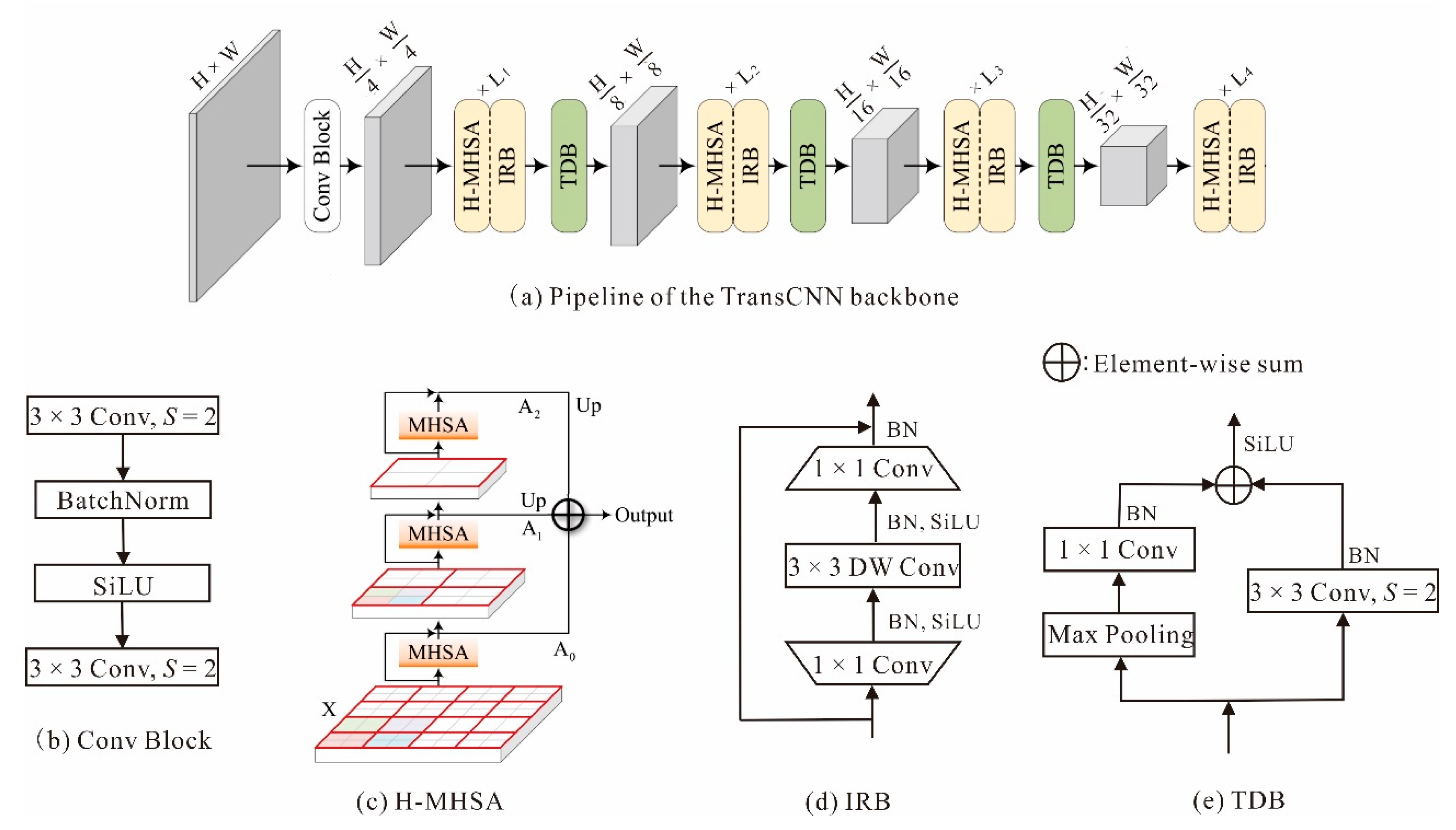
2.2. A Brief Introduction to TransCNN

Inheriting the merits of both transformers and CNNs is a trend in the design of state-of-the-art transformers, such as ConViT, CvT, CSWin [26], TransCNN, and so on. In this study, we opted to use TransCNN as the backbone for deep feature extraction, and the reason behind this is threefold: (1) TransCNN introduces a hierarchical framework for computing MHSA (namely, multi-head self-attention). (2) In order to decrease the computational/space complexity, the commonly used MHSA is replaced by H-MHSA, which has three advantages: (i) modeling global dependencies of the input directly; (ii) having the ability to process large input images with ease; and (iii) being more lightweight than traditional MHSA. (3) One can plug the flexible H-MHSA or the whole TransCNN as a backbone into CNNs instead of using an MLP (Multilayer Perceptron) after MHSA computation for feature enhancement, as in other transformers.
The TransCNN backbone has four basic modules: Patch Embedding, H-MHSA, IRB, and TDB, and their architectures are displayed in Figure 1b–e. Of these modules, Patch Embedding, IRB, and TDB are all CNN-related; here, we focus on the inner workings of H-MHSA, which is a three-step procedure: Firstly, instead of computing attention across all patches/tokens, it is better to group patches into small grids and compute attention within each grid. This operation can capture local relationships and yields more discriminative local representations. Secondly, in order to capture feature relationships in larger regions, we need to merge these small grids into larger ones and compute attention within each new grid by viewing small grids in the preceding step as tokens. Thirdly, this process is iterated to gradually reduce the number of tokens.
Throughout this procedure, we computed MHSA (refer to [27] for algorithmic details) in regions with increasing sizes step by step and naturally modeled the global relationship in a hierarchical manner. This strategy leads to better generalization results, and as each grid at each step only has a small number of tokens, the relevant computational/space complexity is greatly reduced. For example, according to [24], the computational complexity of MHSA is 3NC2 + 2N2C, where N and C are the number of tokens and the feature dimension of each token, respectively, while H-MHSA’s complexity is only 3NC2 + 2NG2C, where G is the size of the small grid, and G2 is much smaller than N.
Note that, here, we used the TransCNN_small model as the backbone; the dimensions of the four transformer-CNN blocks are 64, 128, 256, and 512, respectively; their grid sizes are 8, 8, 8, and 1, respectively; the depths (i.e., the number of repetitions) of each block are 3, 4, 8, and 3. Other hyperparameter settings of TransCNN_small are consistent with those in [24].

2.3. Incorporation of the Sharpness-Aware Minimizer (SAM)

The training procedure for mainstream convolution-free transformer architectures, as mentioned above, relies heavily on extensive pretraining [22] or a variety of strong data augmentations [29], leaving many hyperparameters to tune [22]. When trained from scratch on a regular-sized dataset without using advanced data augmentations, the ViT network and its variants usually yield inferior accuracy to CNNs of similar size. This is because transformer architectures tend to converge at extremely sharp local minima [29]. To address this issue, the sharpness-aware minimizer (SAM), which can explicitly avoid sharp minima, was put forward. Chen et al. [22] pointed out that by explicitly regularizing the loss geometry through SAM, transformer-related models enjoy much flatter loss plateaus and improved generalization regarding accuracy and robustness.
To be specific, SAM seeks to find the parameter w whose neighbors all have lower training loss Ltrain by formulating a minimax objective:
m i n w   m a x     ε 2 ρ L t r a i n w + ε
where ρ is the size of the neighborhood ball. Without loss of generality, here, the l2 norm is used for its strong empirical results, and the regularization term is omitted for simplicity [29]. The exact solution of the inner maximization is as follows:
ε = arg   m a x ε 2 ρ L t r a i n w + ε
As ε is difficult to obtain, we employ an efficient first-order approximation:
ε ^ w = arg   m a x ε 2 ρ L t r a i n w + ε T w L t r a i n w = ρ w L t r a i n w / | w L t r a i n w | 2
Under the l2 norm, ε ^ w is simply a scaled gradient of the current weight w.
After computing ε ^ , SAM updates w based on the sharpness-aware gradient as:
w L t r a i n w | w + ε ^ w
SAM is an optimization algorithm often used in the training of pure transformer architectures. However, we found that it also performed well when training our transformer-CNN combined model.

2.4. Design of the Decoder Module

The TransCNN encoder with SAM can produce discriminative and hierarchical feature representations for semantic segmentation, and seemingly, there is little room for improvement. However, decoding these deep features to produce the optimal change map is also crucial for CD tasks, and to our knowledge, there are few studies that have investigated the significance of this issue. Here, we propose three types of strategies to decode the feature representations derived from the Siamese extension of TransCNN.

2.4.1. Type I STDecoder-CD

The Type I STDecoder-CD architecture shown in Figure 2a is UNet-like [1], but there are five differences in its function:
(1)
The pre-change (t1) and post-change (t2) RS images are input into two branches of the Siamese network simultaneously, and the Siamese network with shared parameters separately extracts bitemporal representations.
(2)
Unlike UNet [6], there are only four blocks attached to each Siamese branch. Before the UNet-like encoder–decoder operation, there is a “Conv Block” layer, and after the encoder–decoder operation, there is an “FCN” layer. The “Conv Block” layer splits the input image into tokens of non-overlapping patches with a resolution of 16 × 16, while the classifier “FCN” interpolates the decoded feature maps by four times and identifies the change of interest from them.
(3)
The encoder’s network architecture (X) is completely different from that of the decoder (Y); the former adopts the Siamese TransCNN structure, and the latter retains the “Conv + BN + ReLU” structure used in UNet.
(4)
A deep supervision strategy was developed to enrich the model capacity with extra regularization. As shown in Figure 2a, during the training process, the loss of each deep supervision is computed independently and is directly backpropagated to intermediate layers. To be specific, outputs of the FCN layer and each decoder block are fed into a plain 3 × 3 convolution layer followed by a bilinear upsampling layer, and then their losses can be computed (in total, there are four losses in the network). In this way, the intermediate layers are effectively trained, and their weights can be suitably updated [12], thus alleviating the presence of the vanishing gradient.
(5)
As shown in Figure 2a, to fuse the hierarchical feature representations XnA and XnB (n = 1, 2, 3, 4), we apply the concatenation method to the top layer of the TransCNN layer and use the subtraction method for the remaining layers. This combination is termed Difference Detector I in this study. Actually, for a Siamese network, the concatenation weight sharing mode lacks focus on change information between the former and later phases, while the subtraction weight sharing mode lacks focus on the former phase information [30], so the best strategy is to combine the two weight sharing modes within one network architecture. However, [30] also warns that if we first apply the subtraction method and subsequently use the concatenation method, there will be a significant drop in accuracy.

2.4.2. Type II STDecoder-CD

As seen in Figure 3, the Type II STDecoder-CD architecture has four components: a Siamese TransCNN backbone, a difference detector, an FPN module, and an FCN layer. A detailed description of the components is provided below.
The idea of Difference Detector II is borrowed from [20]. It is a double convolution module involving two or three data sources: the output tensor of XA, the output tensor of XB, and the output tensor of the previous difference detector, if any. In this way, change information at different stages can be fused to generate more discriminative and informative feature representations.
FPN uses a pyramidal hierarchy of deep convolutional networks to construct feature pyramids with marginal extra cost [31], and it shows significant improvement as a generic feature extractor in several applications, such as object detection and semantic segmentation. FPN consists of a bottom-up pathway and a top-down pathway. For the former, we chose to use the hierarchical difference detector; then, a top-down pathway with lateral connections was developed for building high-level semantic feature representations at all scales; finally, after the layer-wise upsampling and Conv3ReLU operations, these hierarchy semantic representations are fused to generate a new feature representation with the same size and dimension as the first difference detector. Note that, here, we use Conv3ReLU instead of the traditional 1 × 1 convolution widely used in FPN [31] in order to promote nonlinear change responses. Additionally, before the upsampling of the 4th difference detector, the ASPP (atrous spatial pyramid pooling) [32] module is added for the purpose of obtaining several multi-scale receptive fields, which may improve the networks’ ability to handle both large and small changes. The idea for these minor modifications is borrowed from an open-source CD code, which is available at https://github.com/businiaoo/PRCV2021-Change-Detection-Contest-2nd-place-Solution (accessed on 20 February 2022).
Finally, as displayed in Figure 3a, the deep supervision operation is conducted at four different places so that the weights of intermediate layers can be effectively updated.

2.4.3. Type III STDecoder-CD

Intuitively, it is also better to use the transformer decoder to decode the proposed backbone, which is a combined Siamese transformer-CNN architecture.
As displayed in Figure 4a, we first use the “upsampling + concatenation + convolution” operation to fuse the four difference detectors (Difference Detector II). The output of this step is a context-rich feature representation (denoted by M) with a dimension of 240 and with the same size as the first difference detector—1/4 of the original image size. Then, M is split into L visual words, which contain compact high-level semantic information that effectively reveals the change of interest, and each corresponds to one token vector of 240 elements. The relevant calculation process is shown in Figure 4c. The input of the transformer decoder is M, the semantic tokens derived from it are denoted by T, and its output is M’, which is a representation with the same size and dimension as M. Apparently, the purpose of introducing the transformer decoder is to further refine the image features from M to M’. Finally, M’ is sent to the classifier FCN to generate the predicted change map(s).
Traditionally, the transformer encoder and decoder usually come in pairs [27]. However, we only use the transformer decoder here. Actually, the TransCNN module itself can be considered a hierarchical transformer encoder, so it is unnecessary to add an extra one. As displayed in Figure 4b, the decoder in use consists of ND layers of multi-head cross attention (MHCA) and MLP blocks [19] instead of MHSA.
Formally, at each layer l, MHCA is defined as:
M H C A D l 1 ,   T = C o n c a t h e a d 1 ,   , h e a d h W O
and
h e a d j = A t t ( D l 1 W j q , T W j k , T W j v )
where
A t t Q ,   K , V = σ ( Q K T d ) V
In the above equations, W j q ,   W j k ,   W j v ∈ RC×d (C is the channel dimension of the feature map M) are the learnable parameters of three linear projection layers generating Q, K, and V, and d is the channel dimension of the triplet. W O ∈ Rhd×C is a linear projection matrix, and h is the number of attention heads. σ(·) denotes the softmax function running on the channel dimension.
Formally, at each layer l, MLP is defined as:
M L P T l 1 = G E L U T l 1 W 1 W 2
where W1RC×2C and W2R2C×C are linear projection matrices, and GELU is the activation function.
In MHSA, the query, key, and value are derived from the same token embeddings, and its output is also a 1D sequence of tokens. In order to exploit the relation between each pixel in M and the token set T and generate the refined 2D feature M’, here, we consider the MHCA-based decoder. It treats pixels in M as queries and tokens in T as keys and values. In [19], before the decoding operation, the token embeddings derived from the feature map generated by FCN are first sent to a transformer encoder to obtain compact high-level semantic tokens, but here, we assume that the token embeddings (T) derived from the global context-rich M are directly available to MHCA.
Note that in Figure 4b, ND is set to 1, and the number of heads of MHCA = 8. In Figure 4c, the token length L = 16, and the token dimension C = 240. Other hyperparameter settings are consistent with those in [19].

2.5. The Loss Function

In practical applications of CD, the number of unchanged pixels is often much greater than that of changed ones. At the suggestion of [11], one way to alleviate the impact of sample imbalance is to introduce a hybrid and weighted loss function. Here, we consider the combination of Focal loss and Dice loss [1].
The hybrid loss function (L) can be formulated as follows:
L = L d i c e + L f o c a l
Dice loss (Ldice, see below) attaches similar importance to false negatives and false positives, and it is effectively immune to the sample-imbalance issue [33].
L d i c e = 1 I + ε U I + ε
I = 1 N t i y i   and   U = 1 N t i 2 + y i 2
where the smoothing factor ε is an extremely small number (here, ε is set to 1e-7); 0 ≤ y i ≤ 1 is the predicted value processed using the sigmoid/softmax activation function; and t i is the ground-truth value, which is either 0 or 1.
L f o c a l loss is defined as:
L f o c a l p t = α t 1 p t γ log p t
where p t is the probability that the model predicts for the ground-truth object. Focal loss adds 1 p t γ as a modulating term to the standard cross-entropy loss so that it can focus on learning hard/misclassified samples. Setting γ > 0 reduces the relative loss for well-classified samples ( p t > 0.50), putting more focus on hard, misclassified samples. At the same time, Lfocal gives high weights to the rare class and small weights to the dominating or common class. These weights are referred to as αt. In this study, we empirically set γ = 2, and αt = 0.45.
Because the sigmoid/softmax function, which maps any real values to the range [0, 1], has already been embedded in the loss functions Lfocal and Ldice, we did not end our algorithmic program with the sigmoid or softmax statement in order to avoid the vanishing gradients caused by repetitive normalization [1]. However, we made the sigmoid/softmax function available again when calculating the evaluation metrics in order to scale all of the predicting data between 0 and 1.

2.6. Evaluation Metrics

The FCN module shown in Figure 2 is a single-class object classifier, and it produces only one change map for each input image pair. After the change map is normalized between 0 and 1 using the sigmoid/softmax function, we need a binarization threshold defining whether a certain pixel in it is changed or not. In order to maximize precision and recall at the same time or keep a balance between them, here, the threshold is manually set to 0.70 or so.
By comparing the binarized change map and ground truth, four metrics were used to validate the effectiveness and accuracy of the proposed methods, which are: precision, recall, F1 score, and IOU. Their formulas [1] are respectively given below:
precision = T P T P + F P
recall = T P T P + F N
F 1 = 2 p r e c i s i o n r e c a l l p r e c i s i o n + r e c a l l
IOU = T P / ( F P + T P + F N )
where TP, FP, and FN denote all classes’ total number of true positives, false positives, and false negatives, respectively.

3. Results

3.1. Implementation Details

We implemented STDecoder-CD as well as the relevant comparative experiments using the Pytorch framework, which is open source. We conducted these experiments on a single NVIDIA Tesla V100 with 32 GB of GPU memory and trained for 200 epochs to make the model converge. We trained the relevant models from scratch, and the batch size was set to 4 for input images with a size of 512 × 512 and to 8 for images with a size of 256 × 256. The SAM optimizer was applied during the training phase. It computes the regularized “sharpness-aware” gradient, which is used by the underlying optimizer. Here, the initial learning rate of SAM was set to 0.1, and the underlying optimizer was SGD with momentum = 0.9. Validation was performed after each training epoch, and the best model on the validation set was saved in .pt format and used for evaluation on the test set. In addition, we applied online data augmentation to the input image patches, including flip, rotate, rescale, histogram matching, Gaussian blur, crop, normalization, shuffle, and so on. Because the “CD_ Data_GZ” dataset is too small to fit the experimental models, we added a transfer step here. To be specific, before training on CD_Data_GZ, we initialized the STDecoder-CD series models using weights pretrained on the PIESAT-CD dataset instead of randomly initializing them. In theory, this step helps our neural networks reach better and more robust classification performance on CD_Data_GZ and reduces the risk of over-fitting.

3.2. Comparison and Analysis

3.2.1. The Performance of the Proposed Models

In this section, we compare the CD performance of our STDecoder-CD (Types I, II, and III) with several existing SOTA (state-of-the-art) methods:
(1)
FC-Siam-Diff [6] is a feature-difference method, which extracts multi-level features of bitemporal images from a Siamese UNet architecture, and their difference is used to detect changes.
(2)
STANet [5] is a Siamese-based spatial–temporal attention network for CD. Note that STANet is fine-tuned on the ImageNet-pretrained ResNet-18 model.
(3)
IFN [12] is a multi-scaled feature concatenation method. It fuses multi-level deep representations of bitemporal images with image difference representations by means of attention modules for change map reconstruction. It uses pretrained VGG16 as the backbone network.
(4)
ChangeSTAR [17] is a multi-task architecture for joint semantic segmentation and object change detection. It can reuse any deep semantic segmentation architecture via the elaborately designed ChangeMixin module. ChangeSTAR uses a pretrained deep network (ResNet101) as the encoder. In this analysis, we set the number of iterations to 5600, and the batch size was set to 4 for input images with a size of 512 × 512 and to 16 for images with a size of 256 × 256. The SGD optimizer with momentum = 0.9 and weight_decay = 0.0001 was used during the training process.
(5)
SNUNet-CD [13] uses a densely connected (NestedUNet) Siamese network for change detection.
(6)
SiUNet3+-CD [1] is a Siamese UNet3+-based CD network architecture. Note that SiUNet3+-CD uses the GN (Group Normalization) layer to normalize the inputs to a hidden layer so that the batch size can be set as small as possible [5] in conditions of insufficient computational resources. At the suggestion of [1], the maximum epoch of iterations was set to 70, and the original learning rate was 1 × 10⁻³.
(7)
BIT [19] is a transformer-based CD method. It uses a transformer encoder–decoder network to enhance the context information of CNN features via semantic tokens followed by feature differencing to obtain the change map.
(8)
ChangeFormer [20] is a transformer-based Siamese network for CD. It uses a hierarchical transformer encoder in a Siamese architecture with a simple MLP decoder. We downloaded the pretrained model of ChangeFormer from http://www.dropbox.com/s/undtrlxiz7bkag5/pretrained_changeformer.pt?dl=0 (accessed on 20 February 2022).
To enable a fair comparison, whenever possible, we used the reported performance from the corresponding publications. Otherwise, if not specified, we re-implemented the algorithms based on public codes or using our own Python codes with parameter settings consistent with the relevant references. The same online data augmentation strategy (as mentioned in Section 3.1 was applied to all of the compared methods.
There are several important observations from Table 1:
On the CDD dataset, the BIT model with the pretrained ResNet as its backbone achieves the best CD performance in terms of F1 score, IOU, precision, and recall metrics. FC-Siam-Diff, STANet, and SNUNet-CD have the worst performance. The CD accuracies of our three proposed models, especially Type I STDecoder-CD, are very competitive: their F1 scores and IOUs are all above the average levels of 0.8853 and 0.7999 by a large margin, although there are no pretrained parameters involved in the training process. In addition, as illustrated in Figure 5, compared with the visualization results of the compared methods, our proposed STDecoder-CD series models successfully returns the changed areas with relatively complete shapes/boundaries, high object internal compactness, and fine details. In particular, they are able to identify each slightly changed object with a clear and separated boundary, whereas other methods, except for SiUNet3+-CD, often clump several small changes together. Although ChangeSTAR and BIT have higher values for most of the quantitative metrics in Table 1, our models could show better visual performance in practical applications.
On the PIESAT-CD dataset, our proposed methods achieve substantially higher accuracies when compared to others, including the FCN-based methods (FC-Siam-Diff, ChangeSTAR, SNUnet-CD, and SiUNet3+-CD), CNN + Attention-based methods (e.g., IFN, and STANet), CNN + transformer-based method (BIT), and pure transformer-based method (ChangeFormer). Although many of the PIESAT-CD image pairs are not accurately labeled, the F1 scores achieved by STDecoder-CD are still above the 85% level commonly recommended for industrial applications. As shown in Figure 6, change masks generated by STDecoder-CD preserve the actual shapes of changed objects with complete and separated boundaries, even when there are misregistration errors and missing objects in the labels. On the other hand, the compared methods, including the ones pretrained on a general-use dataset such as ImageNet, often produce false alarms, fragmentized boundaries, and clumped masks. We can also find that, relative to Types II and III, the Type I model obtains a slightly better CD performance on both quantitative metric evaluation and visual comparison.
On the CD_Data_GZ dataset, STDecoder-CD, especially its Type II model, still outperforms other state-of-the-art CD methods. The FCN-based methods (SNUNet-CD, ChangeSTAR, and SiUNet3+-CD) also perform well in this case. As shown in Figure 7, the output images returned by STDecoder-CD series models still retain the best visual quality, and they are less prone to errors due to edges and small objects. In other words, our proposed methods can achieve a good generalization capacity on small datasets by initializing the model parameters using parameters pretrained on PIESAT-CD, so it would be greatly helpful in engineering applications. Note that we also tested the classic transfer learning strategy (1: initialize the weights of the Siamese TransCNN encoder using weights pretrained on PIESAT-CD; 2: freeze these pretrained weights in the encoder part so that only the rest of the weights in the decoder part will be used to compute loss and be updated by the SAM optimizer) on STDecoder-CD, but the performance is very poor. This may be due to the lack of truly representative samples in the PIESAT-CD dataset or due to the limited sample numbers used for transfer.

3.2.2. Efficiency Evaluation

As shown in Table 2, the proposed STDecoder-CD series models have a relatively large number of trainable parameters, but fortunately, their FLOPs (i.e., floating point operations) remain low. That is, STDecoder-CD (especially the Type I model) can maintain a good trade-off between computational complexity/time and accuracy. On the contrary, although some of the compared methods (e.g., SiUNet3+-CD and SNUNet-CD) can provide an acceptable CD performance, the high computational cost limits their real-world applications. Although FC-Siam-Diff and STANet have much lower parameters and FLOPs, their prediction accuracies are worse. ChangeSTAR and ChangeFormer have slightly higher FLOPs, and their CD performance is inferior to STDecoder-CD as well. Here, BIT is an exception: it has smaller trainable parameters and FLOPs with the assurance of accuracy.
However, we must admit that training STDecoder-CD with the SAM optimizer needs a second round of forward/backward propagations to update ε, and this will lead to around 2× computational cost per update. This may be the main disadvantage of the proposed models, and the best way to address this problem is to apply the transfer learning strategy like BIT does, and it may be better to pretrain the singular TransCNN module on large CV (i.e., computer vision) datasets such as ImageNet and then freeze these pretrained weights within TransCNN. This will be carried out in our future work.

3.2.3. Ablation Studies—Testing on the PIESAT-CD Dataset

To verify each decoding component’s contribution to STDecoder-CD, we designed three ablation experiments on the PIESAT-CD dataset as follows:
The Type I decoder will become unavailable if we ablate any components from it, so in order to verify each component’s significance, we chose to adopt the replacement strategy instead of the ablation strategy. Here, we replaced Difference Detector I, as shown in Figure 2, with Difference Detector II, as shown in Figure 3 and Figure 4.
Likewise, there seem to be no independent and separable components in the Type II decoding architecture. As shown in Figure 8b, here, we replaced the right half of the FPN module with the Type I decoder so as to verify which of the two fusion methods, i.e., one that takes the “many-to-many” strategy to fuse the multi-scale deep features and one that takes the “many-to-one” feature fusion strategy, is much more efficient in enhancing the CD performance. Note that the Type II decoder introduces deep supervision after each feature fusion operation, but in order to keep the workflow consistent with the FPN’s (see Figure 8a) and make a fair comparison, here, we introduce deep supervision only after the Y1de block.
For the Type III decoder, an actual ablation experiment can be conducted by removing the transformer decoding component in Figure 4a.
The parameters of the three networks are the same during the training process, and the relevant experimental results are summarized in Table 3 below, from which we can derive the following observations:
(1)
For the Type I decoder, the CD performance of Difference Detector II is only slightly better than that of Difference Detector I in terms of recall, F1 score, and IOU, but the parameters of the former are 10.95M higher than the latter. This implies that the advantage of Difference Detector II is not obvious. Guo et al. [30] further pointed out that the CD accuracy derived from Difference Detector I is several percentage points higher than that derived from the SC or SD detector. Herein, the SC detector only uses Siamese concatenation operations to fuse the hierarchical deep features, and SD only uses Siamese subtraction operations for fusion. Thus, jointly considering the efficiency, accuracy, and robustness, Difference Detector I is still the optimal option for the Type I decoder.
(2)
For the Type II decoder, the CD performance using the “many-to-one” strategy is slightly better than the “many-to-many” strategy in terms of precision, recall, F1, and IOU. One possible reason for this observation is that: the “many-to-one” strategy involves more Conv3ReLU operations, so it can enrich the representation of feature information. In addition, the “many-to-one” strategy can preserve the feature diversity by integrating the hierarchical deep features into a singular feature vector using a parallel architecture, whereas the “many-to-many” strategy processes the hierarchical features in series. Shifting from parallel to series might result in loss of information and the destruction of feature diversity. Moreover, the absence of deep supervision on Y2 and Y3 in Figure 8b may also hurt the accuracy of the “many-to-many” strategy.
(3)
In the BIT model [19], the transformer decoder (MHCA) was successfully used as a decoder to enhance the original features with context-rich tokens by modeling the long-range dependencies. However, as displayed in Table 3, the CD performance of Type III without MHCA is slightly better than the original Type III with it, although the difference is not large. This implies that the transformer decoder is not essential to Type III STDecoder-CD. One possible reason for this observation is that: the deep features generated by TransCNN itself are context-rich, and there may be no need to guide the network to model the long-range relations again using MHCA. On the other hand, if the original features are derived from CNNs, which only take into account the local spatial context at different levels, it is highly recommended to introduce MHCA as the decoder. In addition, unlike FPN, the Type III decoder lacks a hierarchical design; as shown in Figure 4a, it directly concatenates the multi-scale encoding features together, thereby producing sub-optimal results.
Note that it is not necessary to display the visualized results of these experiments because there is no significant improvement in the accuracy values in Table 3.

4. Discussion

A good design of a decoder plays an important but often overlooked role in improving the final change detection performance. However, efforts to investigate the effect of different decoding strategies are unexplored in the current literature. This is a challenging topic that warrants separate studies. Different from existing methods, STDecoder-CD pays particular attention to the significance of the decoder, and in our opinion, there are several meaningful aspects worth discussing, which are listed in the following paragraphs.
First, at the center of STDecoder-CD is the powerful change feature extractor: TransCNN. As shown in Figure 1, because of the patch embedding operation, the maximum size of the hierarchical feature maps is only H/4 times W/4—a quarter of the original image size (H × W)—which implies that there is a significant loss of spatial information for subsequent decoding and classification processes. However, TransCNN still has a certain capability to trace small changes and narrow-shaped objects, as shown in Figure 5, Figure 6 and Figure 7, and it outperforms the other state-of-the-art CD methods, as shown in Table 1. In addition, because the three decoding strategies have limited impact on the performance of STDecoder-CD, we can conclude that TransCNN contributes most to the success of our algorithm.
Second, the CD performance of STDecoder-CD is not completely free from the influence of the decoding strategies. For example, a slight downward trend in accuracy metrics and visual quality is visible from Type I to Types II and III. A slight upward trend in the computational efficiency from Type I to Types II and III can also be found in Table 2. Experimental results show that the Type I decoder can obtain finer change details than Types II and III, possibly due to its multi-scale design and the wide use of deep supervision.
Third, the feature extraction ability of TransCNN is so powerful that it might conceal the contribution from the decoders. If so, the importance of the decoder in Siamese CD networks may be underestimated. For example, BIT and the Type III model use the same decoder (i.e., cross-attention, the core part of the transformer decoder) to enhance the original features with the context-rich tokens by modeling their relations. In Table 3, the CD performance of Type III STDecoder-CD is only suboptimal, whereas Chen et al. [19] verified that the achieved performance of BIT with the cross-attention decoder is even better than BIT without it. This implies that, in some other cases, a well-designed decoder can play a more important role in identifying changes in objects.
Fourth, it is demonstrated that our model has good generalization ability and transferability from PIESAT-CD to CD_Data_GZ, but it does not generalize well from CDD to CD_Data_GZ. CD_Data_GZ differs from CDD in terms of the sensor type and definitions of change. Therefore, in a follow-up study, it is necessary to create a general pretrained model for STDecoder-CD using sufficient training samples covering different changing objects, imaging conditions, and sensor types.
Fifth, one ongoing challenge in the use of STDecoder-CD for change detection is how to automatically set the threshold for binary “change versus non-change” classification. If the threshold value is large, precision is higher while recall is lower, and vice versa. In this study, the optimal threshold values (~0.70) were determined through a process of trial and error. In the future, we plan to modify the “FCN” module of the three decoders as a two-class object classifier so that the threshold values can be determined automatically by the “argmax” function in Python/Pytorch.
Sixth, compared to other SOTA models, STDecoder-CD has obvious advantages in terms of accuracy metrics, visual quality, and generalization capacity. It has disadvantages too: e.g., STDecoder-CD is very data-hungry, and long training epochs are required for good convergence. To ease the effort of acquiring high-quality annotation data and reduce the training time, Hassani et al. [34] developed a non-“data hungry” transformer termed CCT (Compact Convolutional Transformer), which can perform head-to-head with state-of-the-art CNNs on small datasets, often with better accuracy and fewer parameters. For future research, we are planning to replace the H-MHSA module in TransCNN with CCT so as to make the model more lightweight, more robust to small datasets, and more competitive in engineering applications.
Seventh, our new findings that differ from previous studies include: (1) Siamese TransCNN is a powerful change feature extractor; (2) different decoding strategies can moderately affect the final CD performance; (3) presumably due to the multi-scale design, the performance gain yielded by the Type I or Type II decoder is significantly larger than that obtained with the Type III decoder; (4) the transformer encoder and decoder usually come in pairs, and using the transformer decoder alone, like Type III STDecoder-CD, does not produce optimal results; (5) the proposed decoding architectures are stable and not sensitive to ablation studies; and (6) for small datasets, the introduction of transfer learning is necessary, but it is better to initialize all of the parameters of STDecoder-CD using pretrained weights and then fine-tune them, rather than freezing and only initializing the encoder part. With these innovations, the STDecoder-CD series model can be greatly helpful in real-world applications; for example, it can assist in land use/cover management, urban planning, and monitoring of landslides. In particular, the large-scale application of our methodology is also feasible due to its ability to identify small changes and its relatively low computational complexity.

5. Conclusions

This study puts forward three different types of decoder design schemes to decode a Siamese TransCNN-based backbone, namely, the STDecoder-CD series model. Type I STDecoder-CD has a UNet-like decoder. Type II STDecoder-CD is defined by a combination of three modules: Difference Detector, FPN, and FCN, and the encoder and decoder communicate mainly through FPN. Type III refines/updates the existing change feature map by using a transformer decoder with MHCA. We hope that our STDecoder-CD models help in improving the understanding of architecture design in this space.
Using the CDD, PIESAT-CD and CD_data_GZ datasets as benchmarks, a series of comparative experiments and ablation experiments were conducted, and our findings show that:
(1)
Due to its powerful change feature extraction and representation capabilities, the TransCNN-dominated STDecoder-CD model is superior to other compared SOTA methods (STANet, ChangeFormer, BIT, SiUNet3+-CD, etc.) in terms of object location, boundary production, and quantitative metrics evaluation.
(2)
Even though different decoding strategies do not seem to impact the accuracy metrics to a significant level, the proposed STDecoder-CD series architecture is not completely free from the influence of the decoding strategies. The Type I decoding module gives the best CD performance.
(3)
Using the ablation or replacement strategy to modify the three proposed decoder architectures has a limited impact on their CD performance.

Author Contributions

Conceptualization, B.Z. and X.L.; methodology, B.Z. and X.L.; software, B.Z.; validation, X.L. and Y.L.; formal analysis, B.Z., H.W. and P.T.; investigation, B.Z. and X.L.; resources, P.T.; data curation, N.O.; writing—original draft preparation, B.Z.; writing—review and editing, P.T.; visualization, B.Z. and X.L.; supervision, P.T.; project administration, Y.L.; funding acquisition, Y.L. All authors have read and agreed to the published version of the manuscript.

Funding

This research was funded by the Soft Science Research Plan item of Zhejiang Province, China, grant number 2022C35070.

Institutional Review Board Statement

Not applicable.

Informed Consent Statement

Not applicable.

Data Availability Statement

The datasets used in this study are publicly available: CDD is available at http://aistudio.baidu.com/aistudio/projectdetail/882508 (accessed on 20 February 2022); PIESAT-CD is available at https://captain-whu.github.io/PRCV2021_RS/dataset.html (accessed on 20 February 2022); and CD_Data_GZ is available at https://pan.baidu.com/s/12Ln-nCb15YNu1T28pzC0rA (accessed on 20 February 2022).

Acknowledgments

Constructive criticism and helpful review comments on this manuscript were provided by several anonymous reviewers, and the authors would like to thank them here. We also thank Dongsheng Liu in the PIESAT International Information Technology Limited for providing the PIESAT-CD dataset.

Conflicts of Interest

The authors declare no conflict of interest.

References

  1. Zhao, B.; Tang, P.P.; Luo, X.Y.; Li, L.Z.; Bai, S. SiUNet3+-CD: A full-scale connected Siamese network for change detection of VHR images. Eur. J. Remote Sens. 2022, 55, 232–250. [Google Scholar] [CrossRef]
  2. Wiratama, W.; Lee, J.; Park, S.E.; Sim, D. Dual-dense convolution network for change detection of high-resolution panchromatic imagery. Appl. Sci. 2018, 8, 1785. [Google Scholar] [CrossRef] [Green Version]
  3. Wang, M.; Zhang, H.; Sun, W.; Li, S.; Wang, F.; Yang, G. A coarse-to-fine deep learning based land use change detection method for high-resolution remote sensing images. Remote Sens. 2020, 12, 1933. [Google Scholar] [CrossRef]
  4. Peng, D.; Zhang, Y.; Guan, H. End-to-end change detection for high resolution satellite images using improved UNet++. Remote Sens. 2019, 11, 1382. [Google Scholar] [CrossRef] [Green Version]
  5. Hao, C.; Shi, Z. A spatial-temporal attention-based method and a new dataset for remote sensing image change detection. Remote Sens. 2020, 12, 1662. [Google Scholar]
  6. Rodrigo, C.D.; Saux, B.L.; Alexandre, B. Fully convolutional siamese networks for change detection. In Proceedings of the 25th IEEE International Conference on Image Processing (ICIP), Athens, Greece, 7–10 October 2018; pp. 4063–4067. [Google Scholar]
  7. Song, K.; Cui, F.; Jiang, J. An Efficient Lightweight Neural Network for Remote Sensing Image Change Detection. Remote Sens. 2021, 13, 5152. [Google Scholar] [CrossRef]
  8. Jiang, F.; Gong, M.; Zhan, T.; Fan, X. A semi-supervised GAN-based multiple change detection framework in multi-spectral images. IEEE Geosci. Remote Sens. 2019, 17, 1223–1227. [Google Scholar] [CrossRef]
  9. Peng, D.; Bruzzone, L.; Zhang, Y.; Guan, H.; Ding, H.; Huang, X. SemiCDNet: A semi-supervised convolutional neural network for change detection in high resolution remote-sensing images. IEEE Trans. Geosci. Remote 2021, 59, 5891–5906. [Google Scholar] [CrossRef]
  10. Tang, P.; Li, J.; Ding, F.; Chen, W.; Li, X. PSNet: Change detection with prototype similarity. Visual Comput. 2021, 1–10. [Google Scholar] [CrossRef]
  11. Zhang, W.; Lu, X. The spectral-spatial joint learning for change detection in multispectral imagery. Remote Sens. 2019, 11, 240. [Google Scholar] [CrossRef] [Green Version]
  12. Zhang, C.; Yue, P.; Tapete, D.; Jiang, L.; Shangguan, B.; Huang, L.; Liu, G. A deeply supervised image fusion network for change detection in high resolution bi-temporal remote sensing images. ISPRS J. Photogramm. 2020, 166, 183–200. [Google Scholar] [CrossRef]
  13. Fang, S.; Li, K.; Shao, J.; Li, Z. SNUNet-CD: A densely connected siamese network for change detection of VHR Images. IEEE Geosci. Remote Sens. 2021, 19, 1–5. [Google Scholar] [CrossRef]
  14. Chen, J.; Yuan, Z.; Peng, J.; Chen, L.; Li, H.; Zhu, J.; Liu, Y.; Li, H. DASNET: Dual attentive fully convolutional siamese networks for change detection of high-resolution satellite images. IEEE J. Sel. Top. Appl. Earth Obs. Remote Sens. 2020, 14, 1194–1206. [Google Scholar] [CrossRef]
  15. Yang, X.; Hu, L.; Zhang, Y.M.; Li, Y.Q. MRA-SNet: Siamese Networks of Multiscale Residual and Attention for Change Detection in High-Resolution Remote Sensing Images. Remote Sens. 2021, 13, 4528. [Google Scholar] [CrossRef]
  16. Cao, Z.; Wu, M.; Yan, R.; Zhang, F.; Wan, X. Detection of small changed regions in remote sensing imagery using convolutional neural network. IOP Conf. Ser. Earth Environ. Sci. 2020, 502, 1–11. [Google Scholar] [CrossRef]
  17. Zheng, Z.; Ma, A.; Zhang, L.; Zhong, Y. Change is everywhere: Single-temporal supervised object change detection in remote sensing imagery. In Proceedings of the IEEE/CVF International Conference on Computer Vision, Virtual, 11–17 October 2021; pp. 15193–15202. [Google Scholar]
  18. Zheng, Z.; Zhong, Y.; Tian, S.; Ma, A.L.; Zhang, L.P. ChangeMask: Deep multi-task encoder-transformer-decoder architecture for semantic change detection. ISPRS J. Photogramm. 2022, 183, 228–239. [Google Scholar] [CrossRef]
  19. Chen, H.; Qi, Z.; Shi, Z. Remote sensing image change detection with transformers. IEEE Trans. Geosci. Remote 2021, 60, 1–14. [Google Scholar] [CrossRef]
  20. Bandara, W.G.C.; Patel, V.M. A Transformer-Based Siamese Network for Change Detection. arXiv 2022, arXiv:2201.01293. [Google Scholar]
  21. Wu, H.P.; Xiao, B.; Codella, N.; Liu, M.C.; Dai, X.Y.; Yuan, L.; Zhang, L. Cvt: Introducing convolutions to vision transformers. In Proceedings of the IEEE/CVF International Conference on Computer Vision, Virtual, 11–17 October 2021; pp. 22–31. [Google Scholar]
  22. Chen, X.; Hsieh, C.J.; Gong, B. When vision transformers outperform ResNets without pre-training or strong data augmentations. In Proceedings of the International Conference on Learning and Reinforcement (ICLR), Vienna, Austria, 16–17 August 2021; pp. 1–20. [Google Scholar]
  23. Liu, Z.; Mao, H.; Wu, C.-Y.; Feichtenhofer, C.; Darrell, T.; Xie, S. A ConvNet for the 2020s. In Proceedings of the IEEE/CVF conference on Computer Vision and Pattern Recognition, New Orleans, LA, USA, 21–24 June 2022; pp. 1–15. [Google Scholar]
  24. Liu, Y.; Sun, G.; Qiu, Y.; Zheng, L.; Chhatkuli, A.; Gool, L.V. Transformer in convolutional neural networks. arXiv 2021, arXiv:2106.03180. [Google Scholar]
  25. Srinivas, A.; Lin, T.Y.; Parmar, N.; Shlens, J.; Abbeel, P.; Vaswani, A. Bottleneck transformers for visual recognition. In Proceedings of the IEEE/CVF Conference on Computer Vision and Pattern Recognition, Nashville, TN, USA, 20–25 June 2021; pp. 16519–16529. [Google Scholar]
  26. Dong, X.; Bao, J.; Chen, D.; Zhang, W.M.; Yu, N.H.; Yuan, L.; Chen, D.; Guo, B.N. Cswin transformer: A general vision transformer backbone with cross-shaped windows. arXiv 2021, arXiv:2107.00652. [Google Scholar]
  27. Dosovitskiy, A.; Beyer, L.; Kolesnikov, A.; Weissenborn, D.; Zhai, X.H.; Unterthiner, T.; Dehghani, M.; Minderer, M.; Heigold, G.; Gelly, S.; et al. An image is worth 16x16 words: Transformers for image recognition at scale. In Proceedings of the International Conference on Learning and Reinforcement (ICLR), Vienna, Austria, 3–7 May 2021; pp. 1–22. [Google Scholar]
  28. d’Ascoli, S.; Touvron, H.; Leavitt, M.L.; Morcos, A.S.; Biroli, G.; Sagun, L. Convit: Improving vision transformers with soft convolutional inductive biases. In Proceedings of the 38th International Conference on Machine Learning, San Diego, CA, USA, 18–24 July 2021; pp. 2286–2296. [Google Scholar]
  29. Foret, P.; Kleiner, A.; Mobahi, H.; Neyshabur, B. Sharpness-aware minimization for efficiently improving generalization. In Proceedings of the 9th International Conference on Learning Representations, Vienna, Austria, 3–7 May 2021; pp. 1–12. [Google Scholar]
  30. Guo, Y.; Long, T.; Jiao, W.; Zhang, X.; He, G.; Wang, W.; Yan, P.; Xiao, H. Siamese Detail Difference and Self-Inverse Network for Forest Cover Change Extraction Based on Landsat 8 OLI Satellite Images. Remote Sens. 2022, 14, 627. [Google Scholar] [CrossRef]
  31. Seferbekov, S.; Iglovikov, V.; Buslaev, A.; Shvets, A. Feature pyramid network for multi-class land segmentation. In Proceedings of the IEEE Conference on Computer Vision and Pattern Recognition Workshops, Salt Lake City, UT, USA, 18–23 June 2018; pp. 272–275. [Google Scholar]
  32. Chen, L.C.; Zhu, Y.; Papandreou, G.; Schroff, F.; Adam, H. Encoder-decoder with atrous separable convolution for semantic image segmentation. In Proceedings of the European Conference on Computer Vision, Munich, Germany, 8–14 September 2018; pp. 801–818. [Google Scholar]
  33. Li, X.; Sun, X.; Meng, Y.; Liang, J.; Wu, F.; Li, J. Dice loss for data-imbalanced NLP tasks. arXiv 2019, arXiv:1911.02855. [Google Scholar]
  34. Hassani, A.; Walton, S.; Shah, N.; Abuduweili, A.; Li, J.; Shi, H. Escaping the big data paradigm with compact transformers. arXiv 2021, arXiv:2104.05704. [Google Scholar]
Figure 1. Illustration of TransCNN (modified after [24]). DW Conv represents depthwise separable convolution; TDB: Two-branch Downsampling Block; IRB: Inverted Residual Bottleneck; × Li means that the H-MHSA + IRB block is repeated Li times; S denotes the stride of the convolution; H and W denote the height and width of the input image, respectively; SiLU is the nonlinear activation function.
Applsci 12 07903 g001
Figure 2. Flowchart of the Type I STDecoder-CD architecture. The legends in this figure are consistent with those in Figure 1 if not specified.
Applsci 12 07903 g002
Figure 3. Flowchart of the Type II STDecoder-CD architecture. The legends in this figure are consistent with those in Figure 1 and Figure 2 if not specified.
Applsci 12 07903 g003
Figure 4. Flowchart of the Type III STDecoder-CD architecture. Note: (b,c) are modified after Ref. [19]. The legends in this figure are consistent with those in Figure 1, Figure 2 and Figure 3 if not specified.
Applsci 12 07903 g004
Figure 5. Visualized results of STDecoder-CD series models and the compared methods on the CDD dataset. Red rectangles represent typical false negatives (the missing portions). Note: due to limited space, we could not show the prediction results of all of the algorithms listed in Table 1.
Applsci 12 07903 g005
Figure 6. Visualized results of STDecoder-CD series models and the compared methods on the PIESAT-CD dataset. Red rectangles represent missing annotations in the labels. Red ellipses highlight typical false alarms. Note: due to limited space, we could not show the prediction results of all of the algorithms listed in Table 1.
Applsci 12 07903 g006
Figure 7. Visualized results of STDecoder-CD series models and the compared methods on the CD_Data_GZ dataset. Note: due to limited space, we could not show the prediction results of all of the algorithms listed in Table 1.
Applsci 12 07903 g007
Figure 8. (a) The “many-to-one” feature fusion strategy; (b) the “many-to-many” strategy. The legends in this figure are consistent with those in Figure 1, Figure 2, Figure 3 and Figure 4 if not specified.
Applsci 12 07903 g008
Table 1. Performance comparison on CDD, PIESAT-CD, and CD_Data_GZ datasets.
IndexPrecisionRecallF1 ScoreIOU
Method CDD
FC-Siam-Diff0.78300.62600.69200.5335
STANet0.85200.89200.87200.7723
IFN0.95000.86100.90300.8237
ChangeSTAR *0.92800.91320.92050.8527
SNUNet-CD * 0.91400.84200.87650.7802
SiUNet3+-CD0.94700.87000.90690.8296
BIT *0.95060.94170.94610.8978
ChangeFormer0.93630.85490.89380.8079
Type I (ours) *0.94390.89720.92000.8517
Type II (ours) *0.92900.87610.90170.8210
Type III (ours) *0.93130.88230.90610.8284
MethodPIESAT-CD
FC-Siam-Diff *0.76900.48570.59540.4239
STANet *0.79030.76600.77800.6366
IFN *0.43890.45800.44830.2889
ChangeSTAR *0.82980.82020.82500.7021
SNUNet-CD * 0.78390.80620.79490.6596
SiUNet3+-CD *0.80090.77970.79010.6531
BIT *0.85300.80470.82810.7067
ChangeFormer0.88470.76860.82250.6986
Type I (ours) *0.88510.83160.85750.7506
Type II (ours) *0.88470.82940.85620.7485
Type III (ours) *0.87100.83500.85260.7431
MethodCD_Data_GZ
FC-Siam-Diff **0.72180.65010.68410.5198
STANet *0.78680.16140.26790.1547
IFN *0.46440.48590.47490.3114
ChangeSTAR *0.86550.70010.77410.6314
SNUNet-CD ** 0.77080.77220.77150.6280
SiUNet3+-CD **0.77250.75500.76370.6177
BIT *0.79900.63160.70550.5450
ChangeFormer *0.69340.51790.59290.4214
Type I (ours) **0.80200.76470.78290.6433
Type II (ours) **0.82160.75130.78490.6459
Type III (ours) **0.78570.72740.75540.6070
Best results are highlighted in bold font. The precision, recall, F1 score, and IOU are averaged over all images in the three testing datasets. * Means our re-implemented results and/or pretrained files. ** Represents that we initialized the models using weights pretrained on the PIESAT-CD dataset.
Table 2. A list of different models’ parameters and FLOPs (when the input image size is 256 × 256).
MethodParameters (M)FLOPs (G)
FC-Siam-Diff1.354.71
STANet16.9312.98
IFN50.7182.26
ChangeSTAR52.5819.53
SNUNet-CD12.0354.77
SiUNet3+-CD27.00216.72
BIT12.4010.59
ChangeFormer29.7521.19
Type I (ours)40.8412.14
Type II (ours)52.4518.20
Type III (ours)53.8918.29
Table 3. The ablation study using the PIESAT-CD dataset.
DecoderParametersPrecisionRecallF1 ScoreIOU
Original Type I40.84M0.88510.83160.85750.7506
Type I using Difference Detector II51.79M0.88290.83570.85870.7523
Original Type II52.45M0.88470.82940.85620.7485
Type II using the “many-to-many” strategy54.95M0.88340.81760.84920.7380
Original Type III53.89M0.87100.83500.85260.7431
Type III without transformer decoder53.16M0.87920.83020.85400.7452
Best results are highlighted in bold.
Publisher’s Note: MDPI stays neutral with regard to jurisdictional claims in published maps and institutional affiliations.

