1. Introduction
Atmospheric turbulence or gusts produce significant deformations when they encounter highly flexible structures such as aircraft wings. These deformations can reach 20% of the wing span in some severe cases. The fuel tanks, which are placed inside the wings, carry a weight of fuel comparable to the oscillating structural components. The current engineering practices for wing design do not include the dynamical effects that the fuel produces within the tanks, which could affect the aircraft design loads. The major experimental tests to identify and verify the dynamic characteristics of the aircraft structure (Ground Vibration and Flight Flutter tests) are limited to small amplitudes and barely excite significant sloshing modes.
In this context, the EU-SLOWD research project [
1,
2] aims to study how much fuel sloshing affects the structural damping of the wing oscillations. One of the main ideas of the SLOWD project is to present a comparable set of experimental and numerical campaigns based on scaled and simplified experiments that could predict some quantitative results up to a full-scale wing experiment, where the amplitudes are large enough to produce relevant sloshing effects. During this project, a large number of experimental and numerical studies have been produced.
Despite that violent sloshing is a highly nonlinear phenomenon, some early theoretical approaches to the problem are found in this field; see, for example, the classical references [
3,
4,
5]. In terms of experimental results, the first studies were based on a partially filled tank attached to an oscillating cantilever beam, which demonstrated that the extra damping that appears is due to the sloshing motion; see [
6,
7]. This extra damping was measured in terms of decrements on the tip beam acceleration. In this experiment, a baffled water tank was mounted on a 2.35 m cantilever which is broadly representative of a wing and its fuel tanks. The cantilever is forced into a deflected shape and suddenly released, such that the free beam decaying oscillations are recorded by several accelerometers while the forces between the beam and the tank are measured by load cells. Based on these promising results, and taking into account that the damping of the tank acceleration and the vertical sloshing force that interacts between the liquid and the tank are the two most relevant outcomes from the experiment, a similar Froude multi-scale campaign was carried out at the Model Basin Research Group Sloshing Laboratory of the UPM in Madrid, Spain; see [
8]. In this work, an experimental methodology is developed to quantify the kinematics and the sloshing forces on a vertical Single Degree Of Freedom (SDOF) tank excited with real wing accelerations. These experiments confirmed again that the fluid sloshing increases the global damping of the system notably, finding that the slosh-induced damping force includes an inertial term and a dissipative term. An important conclusion obtained was that the time shift between the force impacts and the tank maximum displacement is a very relevant magnitude in fluid-induced energy dissipation. Another experimental campaign based on a release test of a vertically vibrating structure again confirmed the additional damping created by the sloshing motion; see [
9]. These experiments show that the damping depends on the amount of fluid in the tank and the initial maximum acceleration. In this experiment, where the tank is not guided vertically and the structural damping is reduced, three distinct response regimes corresponding to different motions of the fluid are observable during the transient decay, the starting one being the most important in the overall energy dissipation. Other experimental campaigns where the tank is moved periodically with different amplitudes and frequencies and the sloshing force and the tank kinematics are measured are performed in [
10,
11,
12].
The other methodology used to study violent sloshing flows is the computational one, where different numerical techniques can be applied. Recent relevant studies based on different mesh-based techniques, such as the finite volumes proposed in [
13], or the particle finite element method (p-FEM) [
14] are examples of the different strategies used to tackle different sloshing problems. However, in this work, the Lagrangian meshless method Smoothed Particle Hydrodynamics (SPH) has been used instead to discretize the liquid phase of the problem, assuming that the gas phase plays a negligible role. The SPH method has been widely extended to different applications in the past decades, such as free surface flows [
15]. The SPH technique already has an important background solving complex computational engineering problems [
16,
17], which includes fluid–structure interaction problems [
18] and violent sloshing problems in the presence of complex geometries [
19]. Recently, a thorough validation on sloshing flows occurring in tanks of different shapes has been carried out by Green [
20]. A very focused application of a reformulated and adapted version of weakly compressible SPH to this violent problem was performed by [
21,
22]. In this two-part paper, a tank-fluid system is first periodically excited with a prescribed law of motion, and the nonlinear features are observed. The force between the wall and the fluid and the global energy balance are both computed. Then, a validation against experimental results using a fluid–structure interaction formulation is carried out in the second part of the work. After this work, SPH can be considered an efficient and accurate methodology when compared to mesh-based methods to simulate free surface flows, and particularly violent sloshing flows.
A very detailed study on the initial stages of this sloshing problem where the Rayleigh–Taylor instability alters the free surface is performed in [
23]. Normally, the Rayleigh–Taylor instability (RTI) appears when the density gradient due to the presence of different fluids and gravity is opposed. This situation is present at the initial stages of our problem, when the two different fluids are confined and the tank is accelerated upwards. In our case, the light fluid overlies a heavier fluid by the action of gravity, but the RTI is developed when a larger acceleration than gravity is applied to both fluids in the direction opposite to the force of gravity. As explained before, the density gradient is opposed to the difference between the inertial force and gravity. In order to understand what is causing the initial free surface deformation, the Rayleigh–Taylor instability can be studied comparing the results from the SPH simulations and other results obtained when the Navier–Stokes equations are perturbed and linearized; see [
23]. Very few SPH approaches [
24,
25] contain a detailed quantitative comparison to other classical numerical formulations where well-established results such as the growth rate of the linear parts of the RTI are monitored.
This paper shows a dual approach, experimental and numerical, to the study of the violent vertical sloshing flows described above in the context of aeronautics applications. This paper will be focused on the comparison of both methodologies in terms of the most primitive results obtained from both approaches. Consequently, the visualization and kinematics of the flow evolution will be compared, and the physical insights of the sloshing force will be deeply studied. The present article is organized as follows: in
Section 2, the process followed to transform the aeronautical problem into a simpler problem is laid out, and is later studied deeply from both an experimental and numerical point of view. In
Section 3, both the numerical and the experimental methodologies are explained. In
Section 4, the obtained results are presented for both methodologies, applied and compared. Finally, the conclusions are summarized and discussed in
Section 5.
2. Modeling of the Problem
In this section, the general approach to model this complex problem will be explained, where a good number of simplifications are assumed to transform the real aeronautical problem into a simple experimental rig and its corresponding numerical version, both containing the most relevant physics from the original case.
When all the complexity of the industrial case is attempted to be described, a problem where an immiscible multiphase fluid confined inside a deformable moving tank emerges. The tank moves with a trajectory given by the deformations of the aircraft wing, which gives rise to a great number of vibration modes and therefore to complex movement. Both fluids, liquid and gas, are viscous with surface tension between them and initial formation of menisci caused by the walls. The movements of both fluids inside the tank are characterized by high Reynolds numbers, and therefore turbulence and non-linear effects are relevant. The numerical simulations must model those turbulent scales that normally the computational mesh does not resolve. Gravity and inertial forces due to acceleration are also present and especially relevant in this problem. It should also be remarked that a fluid–structure interaction case is faced, where in addition to the possible deformations of the container, there is a two-way interaction between the fluid and the tank through the pressure fields and viscous stresses produced, which makes the dynamics of the tank and those of the fluid clearly coupled.
Given such a number of complexities, if a simple model that contains the physical phenomena that are taking place has to be manufactured, some simplifications need to be assumed:
The tank is manufactured in such a way that very small deformations appear, and then it can be considered as a rigid solid.
Even though the tank moves with complex 6 degrees of freedom (DoF) kinematics inside the wing, the movement in the vertical direction is much larger than in any other, and as a consequence, the tank movement will be simplified to a vertical 1-DoF movement with no rotations.
Despite that the fluid has a 3D movement inside the tank providing a 3D pressure field, 3D computations are very costly in terms of computational time, and the 2D results are accurate enough to obtain good performance (see [
26]); thus, the computational fluid dynamics will be performed using a 2D domain.
Assuming all these simplifications, the fuel tank inside the aircraft wing will be simplified to an experimental rig that consists of a vertically guided tank that is partially filled with liquid and air. An initially deformed spring system generates a decaying oscillating movement in the tank and the confined fluid. A more detailed description of the system is performed in the next
Section 3.1.
3. Methodology Description
The two different approaches, experimental and numerical, give a double perspective that allows a very complete and rigorous analysis of this complex problem. On one hand, the double approach implies comparison of some of the magnitudes that can be obtained independently by both methodologies, but also brings the possibility of testing whether some of the simplifications assumed in the computational framework are justified. On the other hand, both perspectives are complementary as the experimental measures are basically global magnitudes, while the computational approach is able to compute local pressure and velocity values.
3.1. Experimental Approach
In this section, the vertical sloshing experimental setup, which is an improved version of the one used in [
8], is briefly described. The sloshing rig is a 1 degree of freedom system composed of a mechanical guide that allows only vertical motion. This guide is attached to a C-shaped wooden structure that holds the tank. This C-shaped wooden structure is attached to a set of 6 springs (3 on the upper side and 3 on the lower side), each of them having an individual spring constant of
N/m. The lower springs are mechanically embedded to the floor and on the opposite side, the upper set of springs is attached to a metallic plate that acts as a joint between them and the embedded load cell. A photograph of the 1/5 scale experimental setup at the Model Basin Research group sloshing laboratory of the UPM and a simplified outline are both shown in
Figure 1.
The tank dimensions of a scaled experiment with a scale parameter
are:
H for the height and depth,
L for the length and
h for the liquid height. The length
represents the tank height of the aircraft fuel tank. The system is displaced by an initial amplitude
until it is fixed by the action of the pair of solenoids located at the bottom of the setup at
. The permanent solenoids produce a magnetic force until the electrical current is turned on, triggering the release of the structure and the beginning of the oscillatory movement. In
Figure 2, the experimental snapshots of a 50% fill level
water test for
and
are presented. The timeline of the snapshots has been referenced to the wing scale according to the Froude scaling laws (
).
Once the system is released and accelerated upwards, the initial flat free surface is rippled; see, for example,
Figure 2a,b. While several effects cause the initial free surface deformation, the main cause is the meniscus deformation generated at the boundaries but also in those cases where the tank ceiling contains droplets of liquid attached. These droplets can cause a relevant perturbation when falling down from the upper wall and impacting the free surface. These perturbations in the free surface grow as Rayleigh–Taylor instabilities; see
Figure 2c,d. The instabilities grow and form liquid jets that impact the upper wall of the tank (
Figure 2e) producing the first sloshing force peak. The linear growth of these instabilities has been deeply studied in [
23], where the initial stages of an SPH computation are compared to the linear stability analysis of the Navier–Stokes equations in terms of growth rate and mode shape.
For the rest of the test, a violent and turbulent regime is developed where the free surface is fragmented, small bubbles form, splashing occurs and liquid-to-liquid and liquid-to-wall impacts are seen (
Figure 2f). When the sloshing force is lower than the liquid weight, the violence of the sloshing decreases (
Figure 2g), bigger bubbles form and fewer impacts occur. The liquid starts to return to its initial state with moderate liquid impacts to the lateral walls, and it starts to develop a standing wave-like regime (
Figure 2h). It finally restores its initial state displaying a rotary motion that is attenuated over time (
Figure 2i). This general description will be particularized for the two liquids studied in this paper in
Section 4.
In this experimental setup, there are 3 magnitudes that are being measured: acceleration, position and force. The characteristics of the measuring devices can be found in [
8]. The measured signals are all filtered using a fourth-order Butterworth filter with a cutoff frequency of 20 Hz. The uncertainty analysis of the measurements has been performed in [
27].
Once the acceleration, position and force measurements are post-processed, the following magnitudes are derived: the damping ratio, vertical sloshing force and the phase-shift between liquid action and tank motion. These magnitudes are defined in the subsequent subsections.
3.1.1. Damping Ratio,
Following the procedure explained in [
28], the Hilbert transform of the acceleration signal is calculated in order to obtain the envelope function of the decay. By denoting the acceleration signal as
a, the equation reads as:
where
is an imaginary signal that is shifted
in the complex plane from the real signal
. Defining a function
which is the sum of the real and imaginary parts and considering that the envelope function is the absolute value of this sum:
Then, by assuming a linear decay of the signal, the envelope function is equal to:
where
represents the initial acceleration,
is
times the natural frequency of the experiment and
is the damping ratio. The natural frequency
is computed using the mean period, which is obtained as the mean over the number of cycles within the acceleration range
. To calculate the damping ratio
, a linear fitting is performed to the logarithm of the envelope signal in the same acceleration range. An example of this procedure is shown in
Figure 3 for the scale
reference test (water and glycerine tests at 50% and 39% fill level, respectively;
g). The damping ratio
is calculated as the slope of the linear fitting divided by
.
3.1.2. Sloshing Force,
The vertical sloshing force acting on the SDOF system is experimentally calculated following the procedure shown in [
8] for a similar setup. Denoting the load-cell measurement as
, the vertical sloshing force is:
where the solid moving mass
accounts for the masses of the C-shaped wooden structure, tank, mechanical bearing system and attachments. An in-depth explanation of the derivation of Equation (
4) can be found in [
8]. Using the liquid mass
and its initial acceleration due to the tank movement
as characteristic values, the vertical sloshing forces presented in this paper are non-dimensionalized with
.
3.1.3. Phase-Shift,
The phase-shift
is defined as the angle related to the time-shift between the vertical sloshing force peaks
and tank position peaks
y. The first 3 time-shifts
are shown in
Figure 4 for a water test at 50% fill level and
g.
For each time-shift, a phase-shift between the sloshing force is defined and the tank motion as , and the averaged phase-shift for one experiment is the mean over the first 10 phase-shifts.
Keeping the experimental rig constant, this means using the same linear guide, springs, measuring devices, and rest of mechanical auxiliary parts; the parameter space that this problem involves is still large. The dimensional analysis of this problem has already been performed in several papers; see [
8,
27,
29]. The remaining degrees of freedom of the experiment can be listed as:
Sloshing liquid. Changing the liquid that partially fills the tank implies changing the density, viscosity and the surface tension of the dominant fluid.
Initial amplitude . This change implies a different initial acceleration and inertial forces.
Fill level. This change implies varying the liquid mass inside the tank and consequently the mass ratio between the liquid and the solid moving masses.
The global tank dimensions can also be scaled; see [
27].
The variation of these degrees of freedom, which imply the variation of the dominant non-dimensional numbers of the problem in the context of our experimental rig, was thoroughly studied experimentally in [
27] and computationally in [
26], where it was found that the maximum damping is obtained for a 50% filling level, and the sloshing-induced damping ratio increases with the liquid density. Additionally, it has been concluded that the damping ratio increases with the initial amplitude up until a threshold amplitude of
, after which it starts to decrease. No relevant influence on the damping ratio has been reported due to surface tension variation. The damping ratio is unaffected by liquid dynamic viscosity changes if the flow is at high Reynolds numbers.
3.2. Numerical Approach
SPH formulation for free-surface flows can be based on a weakly compressible formulation, in which fluid pressure and density are linked through a barotropic law. Under this assumption, Navier–Stokes equations can be written as:
where
is the material derivative;
is the fluid density;
p the pressure;
the fluid velocity vector (bold letters indicate vector magnitudes) that is defined from the fluid particles position,
;
a generic external volumetric force field F; and
is a surface tension force field.
indicates the stress tensor, which, for Newtonian fluid such as the ones used in the applications of this work, is defined as:
with
being the rate of strain tensor, i.e.,
;
the identity matrix; and
and
the fluid viscosity coefficients, respectively.
Relationship between pressure and density in (
5) is established by means of a linear stiff equation of state (EOS). This allows for adjusting compressibility so that the speed of sound (
) can be artificially lowered [
30]. In a weakly compressible context, the condition to be satisfied corresponds to Mach number
. In this work, this condition is met if
, with
U being the maximum speed in the system, which is taken as the maximum speed of the tank.
Hence, the set of Equations in (
5) become in SPH
where
, and
represents the volume of the neighbor particles
j, defined as
. In the present work, the kernel function, defined as
, is a Wendland C2 kernel with
being used, where
h corresponds to the smoothing length and
to the particle distance.
The dissipation effects due to viscosity are modeled through
, as is the standard in the literature (see, e.g., [
31]). This function is defined as:
An extra numerical term is added to the continuity equation in order to avoid spurious high-frequency pressure oscillations. The model used in this work corresponds to the one developed by [
30], which is known as
-SPH. The function
from this term is defined as:
where
represents the renormalized density gradient, as defined by [
32]. The value for
is set always to 0.1.
Boundaries are modeled according to the numerical boundary integrals approach, as described by [
33]. They are discretized by elements that are defined by geometrical properties, such as their area, normal and tangent. Connectivity between nodes is avoided, allowing a faster and more efficient computation, even though a truncation error is assumed. Lately, some features have been added, and the Shepard factor is now computed geometrically through a semi-analytical approach, improving the stability and robustness of the simulations [
34].
Generally, no-slip boundary conditions should be used for the tank walls. However, when the Reynolds number is around
and greater, the wall boundary layer is thinner than the resolutions tested in the present work. Then, free slip boundary conditions are used on the tank walls instead, even though the expected difference is small, as has been already discussed in [
22].
Time integration is performed by means of a predictor–corrector scheme. Due to the violence of the impacts expected during the simulation, the Courant–Friedrichs–Lewy (CFL) condition is set to 0.1. Several time step constraints are imposed in order to consider all the phenomena involved, taking the minimum of them at every time step:
Simulations have been carried out with the open-source SPH software AQUAgpusph developed by CEHINAV-UPM. As a reference, see, e.g., [
26,
33,
34,
35,
36] for applications done with this software. For further information, and to download the official release of the code, it can be accessed at
http://canal.etsin.upm.es/aquagpusph/. Last access 4 August 2022.
3.2.1. Additional Model Corrections: Particle Shifting and Free-Surface Tracking
The problems covered in this work involve large pressure gradients that can lead to large areas with negative gauge pressures. Under these circumstances, it is possible that numerical cavitation will appear. This is a phenomenon known in SPH as tensile instability, and it is still a great challenge for the method.
There are several sources in the literature that deal explicitly with tensile instability (see e.g., [
37,
38]). Normally, the solution consists of adding a correction term to the momentum equation. Recently, several works have followed a different approach based on the application of the particle shifting technique (PST) introduced by [
39]. Then, in this work a shifting algorithm with a tensile instability correction term will be used, in the same fashion as was proposed by [
40]. As will be shown, this will be enough to avoid numerical cavitation in the simulations. A similar approach to the problem has been followed by [
26] with satisfactory results.
The PST will also improve the accuracy of the scheme, as it will keep the particle distribution regular. However, the system in (
7) needs to be rewritten in an Arbitrary Lagrangian Eulerian (ALE) framework. This implies new terms linked to the particle shifting velocity to be included in the governing equations, as discussed by [
40,
41].
Hence, the particle shifting velocity is defined according to [
40] as:
The shifting velocity points toward the areas where particle distribution is irregular, and its intensity is modulated by the constant
, which is problem dependent. In this work,
. Normally, shifting velocity remains low enough, but an upper limit is established in the present work, being
. Finally, shifting velocity is added to the particle velocity and integrated in time to obtain the corrected position of the particles, such that:
In flows involving a free surface, an additional control is needed for the PST. In this case, a similar approach to the one carried out by [
38] is established:
where
is the region close to the free surface (defined at a distance
h), and a scalar coefficient
is defined such that:
A free-surface tracking algorithm to detect free-surface particles is implemented in accordance to the work developed by [
40,
42]. Those works use thresholds to define different regions depending on how close a particle is from the free surface, based on the minimum eigenvalue (
) of the renormalization matrix, which is defined as:
In a second step, free surface particles can be fully identified, and normal vectors can be found according to the following expression:
As is also discussed by [
40], the presence of solid walls have an influence on the computation of the free surface particles and their associated normal value. In order to have a proper definition of these, eigenvalues at the boundary need to be taken into account in Equation (
16). However, this is not the case when computing shifting velocities from Equation (
13), in which the extension at the boundaries is not considered. Taking into account these details, tips and jets are correctly identified and the simulations remain stable.
3.2.2. Surface Tension Model
A general surface tension field
is added to the momentum equation in Equation (
7) to deal with effects at the interface. These are especially notorious at initial stages of the tests performed in the present work and become crucial to obtain satisfactory results in terms of impacts and lag between fluid and tank motions.
This force has been included in SPH. It is based on the term proposed by [
43], and reads:
where
is the surface tension coefficient.
3.2.3. Sloshing Force and Fluid Structure Interaction
In order to control the tank’s vertical motion, a second-order equation is derived from the application of Newton’s second law to the solid mass
. It is assumed that the forces that are applied to the tank come from three different components, in the same fashion as it has been proposed by [
8]: the spring forces
, the vertical component of the sloshing force coming from the internal fluid action
and the vertical component of the damping force
. The last component is assumed to include all sources of energy dissipation in the system that are not due to fluid slosh. In the present work, these are a Coulomb friction and a viscous friction term, respectively. The resulting equation reads:
where
N represents the Coulomb damping coefficient and
kg/s is the viscous damping coefficient. Finally, the vertical sloshing force
is given, for a Newtonian fluid, by
The first term in Equation (
19) represents the contribution of the pressure forces, and the second term the one from the viscous forces.
corresponds to the tank’s internal walls, and the normal
is defined such that it is pointing outwards. These forces can be computed in SPH, according to the boundary integrals approach, on the boundary elements. The resulting expressions are:
The second term of the viscous force
is taken into account if no slip boundary conditions are enforced. A similar procedure to compute the forces can be found in [
44].
Then, forces obtained according to expressions in Equation (
20) can be applied to Equation (
18) to obtain the vertical motion of the tank.
A fourth-order Runge–Kutta integrator (RK4) is used to obtain accelerations, velocities and positions at each time step. The resulting fields are then applied to the boundary elements in which the tank walls are discretized. This exchange of information is done at every time step. SPH integration algorithm implies much smaller time steps than the ones needed by the RK4 algorithm used for tank motion evolution, and this way it receives updated information every loop, assuring the stability of the coupled system.
4. Results and Discussion
As explained at the beginning of the paper, this work is focused on the physical aspects of the problem, which implies a deep insight into the flow characterization, tank and fluid kinematics (initial jet velocities, final standing wave…) and the sloshing force interchanged between the fluid and the tank.
The sloshing force is measured experimentally according to Expression (
4) and computed numerically according to Expression (
20). Both forces have been accurately compared as part of the code validation in [
22,
26]. The advantage of the computational methodology is among others that the pressure and viscous contributions can be obtained separately. To understand the contributions of these two sloshing force sources, two cases corresponding to two different fluids, water and glycerine, have been studied with the same initial acceleration
, same scale
and same mass ratio
. As these two fluids have different densities, the initial filling level is different for these two cases, (
for water) and (
for glycerine), in order to keep the mass ratio constant. These two fluids, water and glycerine, have the properties shown in
Table 1. As
Table 1 shows, the flows studied have very different Reynolds numbers, which implies a laminar regime in the case of glycerine and a fully turbulent flow for the water. This difference in terms of Reynolds numbers is mainly caused by the large difference in terms of viscosity, and consequently significant differences in the flow behavior and force decomposition between the pressure and viscous parts are observed.
4.1. Comparison of the Flow Evolution: Experimental Visualization versus Numerical Computation
In this subsection, the different stages of the flow from both points of view, numerical and experimental, are compared in order to observe the common characteristics. First, the case of water will be described, and then that of the glycerine in order to remark on the clear differences between both cases. Prior to this work, in [
26], the fact that the extra damping added by the fluid depends on the Reynolds number only when it is below a critical Reynolds value
was observed. Denoting the characteristic Reynolds number for the water and glycerine cases as
and
, respectively, this critical Reynolds number is approximately an order of magnitude lower than the case of water
. Consequently, the Reynolds numbers of the water and the glycerine are placed at two different sloshing regimes
.
4.1.1. Water Case
For the water, three different stages in the flow evolution can be distinguished. We denote as and the instants when the first and the second stage finish and and as the instants where the first and last ceiling impacts are observed.
As displayed in
Figure 5, during the first instants, a ripple generated from the free surface deformation due to the initial meniscus travels horizontally through the free surface from the lateral walls toward the tank center; see a snapshot of this traveling wave in
Figure 5a (
s). This initial stage can be interpreted as a classical evolution of a Rayleigh–Taylor instability. This initial stage finishes with the first fluid–wall impact; see
Figure 5b (
s). In this instant, a four-jet symmetrical image is observed, where two central jets impact the tank ceiling while the other two after traveling up the lateral walls impact at the lateral-top corners.
A chaotic and turbulent regime dominates during the longest part of the experiment. At this stage, the liquid and the gas are chaotically mixed up, making the two fluids difficult to distinguish. The free surface is very fragmented, and air bubbles of different sizes merge and collapse. This second stage finishes at time
. A typical snapshot of this regime can be seen in
Figure 5c (
s).
The last stage shows up after
s, where a mostly compact fluid is observed. The flow transitions to a standing-wave-like behavior that displays some similarities to the rotary sloshing phenomenon observed in [
45,
46], with very small vertical sloshing force variations. The last ceiling impact at time
s is part of this stage. A typical snapshot of this regime can be observed in
Figure 5d (
s).
It can be observed that the 2D computational simulation is able to reproduce the free surface behavior when corresponding snapshots are compared; see
Figure 5. Details such as the double traveling wave that initiates the free surface deformation, the four jets impacting structure and the final standing-wave are well captured by the numerical model.
4.1.2. Glycerine Case
For the glycerine case, the Reynolds number is three orders of magnitude lower, but it can also be distinguished three different stages in the flow evolution, where the same time notation will be used.
As displayed in
Figure 6, during the first instants, no free surface deformation is observed with the exception of the lateral wall meniscus; see a snapshot in
Figure 6a (
s). As demonstrated in [
47], the increment of viscosity decreases the growth rate of the Rayleigh–Taylor instability. It could be assumed that this initial stage finishes with the first fluid–wall impact (
s), which happens at the third tank cycle (first in the case of water). It is worth commenting that three dimensional effects are more present at this first stage in the case of glycerine compared to water, and this can be interpreted by the more dominant role of the viscous stress tensor in this flow.
The second regime of the glycerine is less chaotic and turbulent when compared to the water regime; in this case, jets and traveling boundary layers are clearly observable, and fewer droplets and bubbles appear in the flow. As expected, the higher viscosity makes the liquid more compact and less fragmented. This stage takes approximately the same amount of time compared to the water and also dominates during the longest part of the experiment. As already measured in [
21] comparing water and oil, the damping capacity of a fluid is related to the number of violent impacts, and high viscosity plays an opposite role in this behavior. As a consequence, the more viscous the liquid, the less damping generated. The last ceiling impact is observed at time
s
, which corresponds to the case of water.
After a similar duration to the water
s, the flow transitions to a standing-wave-like behavior. This stage takes less time to relax toward a final flat free surface, with very small vertical sloshing force variations. A typical snapshot of this stage can be observed in
Figure 6d (
s). It could also be observed that in contrast to the water case, the final low-amplitude oscillations of the glycerine case have no impact in the free surface, and the glycerine remains as a block at the bottom of the tank.
An interesting comparison between these two cases can be made in terms of the relative kinetic energy, and this time-dependant number is defined as:
where
and
are the absolute velocity and mass of a fluid particle, respectively, and
is the tank velocity. When the evolution of this relative kinetic energy is plotted for both fluids (see
Figure 7), it is observed that they both start with a similar energy value, but the energy growth for the water is completely different from the glycerine, especially during the first half second of the experiment. The relative energy has been normalized by the initial elastic potential energy introduced in the system
, where
K is the spring constant of the experimental setup. Despite the fact that both flows produce impulsive impacts with the upper and lower tank walls, the higher fragmentation of the water produces larger levels of relative kinetic energy. This high energy stage takes approximately the same time for both fluids
s, after which the impacts are clearly smoothed. In this second stage during the interval 2–3 s, the water free surface continues to be clearly fragmented, while the glycerine seems to be more compact with a more smoothed free surface. After 3 s, the water still impacts the ceiling and wave breaking is observed for the water, while no top impacts are observed and only a combination of standing waves are detected for the glycerine. An interesting difference appears during the last part of the experiment. In the case of the water, the tank movement is more damped and the oscillations are lowered sooner, but a remaining standing wave can be observed for a long time as the viscosity action takes a long time to dissipate its energy. In the case of the glycerine, the tank oscillates a longer time, but the liquid remains a flat block during the whole final part as the viscosity dissipates the standing wave quickly.
In
Figure 8, the tank accelerations of both cases are shown for the same mass ratio and natural frequency. First of all, it can be observed that the matching between the experimental and computational results is very accurate. This validation was already performed in [
26] with an older version of the AQUAgpusph code.
In
Table 2, the damping ratio
defined in
Section 3.1.1 and the time necessary to decrease the tank acceleration to 10% of its initial value
are quantified for the water and glycerine. It is confirmed again that the damping of the water is larger than the glycerine.
In
Figure 9, the vertical sloshing force is plotted for both fluids non-dimensionalized with
, where
is the liquid mass,
is the characteristic angular velocity and
the initial displacement of the tank. Despite a similar plot being shown in previous publications [
26], this new and improved version of the AQUAgpusph code has been able to produce more accurate results than the previous ones. The agreement between the experimental and computational is accurate in both cases. It is interesting to confirm some physical findings that appear in this plot. First, the initial impacts of both cases are quite similar with
N as the mass ratio, and the fluid densities are similar as well. Second, the time required for the water to produce impacts lower that 10% of the initial impact is
s, while the glycerine needs
s to decrease the vertical impacts.
4.2. Flow Kinematics
As explained in
Section 4.1, three stages can be distinguished for both fluids. The fluid kinematics corresponding to the first and last parts will be studied in detail in this section for the case of water. Due to the complexity of the middle part, that part will be studied with other methodologies such as Dynamic Mode Decomposition (see [
48,
49,
50]) in future works. It was also observed that for the glycerine, three-dimensional effects are dominant; consequently, the comparison to the 2D computational approximation is not so clear and will require a future 3D computation.
4.2.1. First Stage
As explained in
Section 4.1, this first stage starts with the relative flow movement inside the tank and finishes with the first ceiling impact. In the case of water, the initial free surface deformation can be studied in terms of impelling jets, which are created symmetrically to the middle vertical plane. In
Figure 10, the free surface obtained by the SPH computation and the one obtained by image processing from experimental snapshots are compared at different time steps before the ceiling impact. The free surface position from the experimental snapshots is extracted by taking into account the decrease in luminosity close to the free surface. The gradient of the luminosity of the snapshot is computed, and the points with the most negative gradient values are extracted. Complex dynamic phenomena are present in the flow, such as traveling wave formation, free surface deformation, central jet formation and the boundary layer evolution on the lateral walls. These are all well captured qualitatively. Although the 2D computational flow shows a very realistic representation of the experimental one, it was observed that the computational region allows the formation of more ripples on the free surface than the real flow is able to diffuse. Although this code has been validated in a typical free surface evolution problem such as the Rayleigh–Taylor one [
23], including surface tension and viscosity, the results obtained here show that when higher velocities and accelerations are present in the free surface, the viscosity and surface tension models should be able to damp these short wavelength instabilities.
The authors would like to underline that in the comparison of the free surface evolution in
Figure 10, a 2D simulation is being compared with a 3D flow; therefore, some differences in terms of flow morphology should be expected. Furthermore, since the tank is moving and the camera is at a fixed position, the angle of view varies with time, and the free surface represented in the experimental snapshots presents some perspective which is not present in 2D simulations.
The symmetric dominant central jets that appear in the free surface have been monitored in terms of relative velocity magnitude for both methodologies, and the quantitative results have been compared in
Figure 11, where the modulus of the velocity has been non-dimensionalized with
. During tank deceleration, a linear growth is observed in the relative jet velocity, and this tendency is well captured by the computations. It is particularly interesting to see that before the final impact, during the whole jet acceleration process, the tank is decelerating. The dispersion of the experimental results when compared to the computational ones is due to the image processing technique, where jet velocity is approximated graphically.
4.2.2. Last Stage: Standing Wave
As explained in
Section 4.1, the last stage of this kind of flow when no violent impacts take place tends toward a typical viscous standing wave in the cases of the water and the glycerine. Two typical snapshots of the standing wave delayed half period for the water can be seen in
Figure 12. The 2D periodic fluid problem can be modeled as a damped mass-spring system [
51], where the mass is equal to the liquid mass, the spring constant is equal to the liquid mass times the square of the characteristic sloshing frequency
, where
k is the wave number associated with the distance between the vertical lateral walls and
is the liquid height, which is 3 cm for water. As in our case, the problem is confined between the lateral walls, and the analytical solution can be only considered an approximation. In this simplified mechanical model, the damping coefficient
depends on the wave number
k and the Reynolds number
; see [
52] for details about the analytical solution. This analytical analogy can only be considered for the case of the water as the glycerine does not satisfy one of the main hypotheses of the analytical solution, which is
.
In
Figure 13, the kinetic energy of the standing wave has been represented using the damped mass-spring model described above and also for the fluid kinetic energy given by Expression (
21). It can be observed that the amplitude of the oscillation is more attenuated for the SPH solution, and this difference can be explained by the presence of surface tension and no-slip boundary conditions on the lateral walls in the SPH simulation. The effect of the lateral walls when viscosity is present was studied in [
23]; in this work, the growth rate variation of the Rayleigh–Taylor instability was quantified by comparison between the confined and the periodic case with the same tank geometry. A lower growth rate value for two different geometries was observed in the confined case when compared to the periodic case for the dominant linear mode. The frequency given by the analytical model matches the SPH solution very well until the flow velocity is extremely low.
4.3. Sloshing Force Decomposition
According to [
8], the sloshing force, either measured in the experiments using Expression (
4) or computed using the pressure and velocity fields by Equations (
19) and (
20), can be divided into three components: the inertial part, which is related to the inertia of the tank motion, and would be present even in the case where there is no relative movement of the liquid in the tank, for example if
; a dissipative contribution that is related to the relative movement of the liquid inside the tank and is responsible for the damping increase of the mechanical system; and a high-frequency contribution of the harmonics with higher frequencies than the natural one. This last contribution is filtered out by using a fourth-order Butterworth filter around the natural frequency of the system.
The part of the force that causes the extra damping in the tank oscillation is clearly the dissipative one; this force
can be modeled as an amplitude multiplied by a shifted cosine function with the natural frequency
. Expanding the cosine, two terms are generated which can be related with the typical force decomposition in velocity and acceleration projections [
53].
where the
and
coefficients can be related with the amplitude
F and the shift angle
by the equations:
The filtered version of the total sloshing force, where the high frequency component is removed, can be expressed using both formulations as:
Another way of understanding the vertical sloshing force is by relating it to the motion of the Center of Mass (CM) of the liquid. Dividing
by
, the following equation is obtained:
Equation (
26) identifies the inertial component of the vertical sloshing force with the tank motion and the dissipative component with the relative motion of the liquid with respect to the tank. In
Figure 14, the non-dimensional relative position of the liquid center of mass
is compared to the term
for both water and glycerine test cases. In this figure, the relative position has been non-dimensionalized with half the liquid height
, which is the initial and final position of the liquid CM relative to the tank. It is worth noting that in
Figure 14, the amplitude of the signals has been extracted from the time domain SPH computation in order to perform the comparison. The overall amplitude of the relative motion of the liquid center of mass matches the amplitude of the dissipative vertical sloshing force as Equation (
26) indicates. Therefore, in order to understand the dissipation of the vertical sloshing problem, it is only necessary to track the relative motion of the liquid center of mass with respect to the tank. This suggests the possibility of using simpler equivalent mechanical models such as the bouncing ball model described in [
54].
In
Figure 15, the filtered sloshing force has been plotted with the direct computation of Expression (
20) and also with both versions of Expression (
25) for the water and glycerine. As can be observed, the agreement between the SPH computation and the derived versions either considering the
and
parameters or the force maxima
F and the shift angle
are both close. This means that the apparently complex sloshing force that comes from a violent and turbulent flow described in
Section 4.1 can be reconstructed using a simple analytical expression based on a cosine function. This fact confirms the possibility of using reduced order models (ROMs) for this kind of problem as has been demonstrated in [
53].
In order to understand the difference in terms of Reynolds numbers and the impact on the sloshing force, the pressure and viscous contributions to the sloshing force have been separated according to Expression (
19) for the water and glycerine. It can be observed that the global sloshing force being similar for both fluids according to
Figure 15, the viscous contribution is much smaller in the case of water when both fluids are compared; see
Figure 16. This is an expected result and confirms the negligible role of the viscous forces when the Reynolds number is high enough
as in the case of water. The pressure forces are on the same order of magnitude for both fluids, being smaller in the case of glycerine. It is also interesting to mention that the viscous forces for the glycerine start having a significant role after
s of simulation. This can be accounted for by the fact that the violent relative movement of the glycerine inside the tank starts after three cycles of the tank and not since the beginning, the first impact being at
s; see
Section 4.1.2. The period of time between
s and
s is the time required for the velocity gradients to grow on the wall boundary layers that flow over the surfaces.
The energy dissipated by the different physical components of the sloshing force can also be studied, where
and
denote the pressure and viscous parts, respectively, and also considering the dissipated energy given by the structural damping force
. These energies are computed using the Expression (
27) and then normalized by
.
In Equation (
27),
F could be any of the three forces mentioned in the previous paragraph. It was observed that the sum of the structural and the pressure forces are above 90%. The energy dissipated by the viscous part of the sloshing force is below 4% in all cases; nevertheless, the glycerine viscous dissipation is notably larger compared to water. The total dissipated energy quantified by these three forces sums to 97.4% for the water and to 96.7% for the glycerine; see
Figure 17. The rest of the dissipation comes from the additional numerical terms that are introduced into the model for stability, such as the
-SPH. Another interesting fact is that in these kinds of experiments, the structural energy dissipated is comparable to the energy dissipated by the fluid in the case of water 55% (structural) versus 42.4% (fluid), but is significantly larger 71% (structural) versus 25.7% (fluid) for the glycerine.
4.4. Pressure Measurements
In this subsection, the possibility of reconstructing the pressure contribution of the sloshing force
as a sum of a discrete number of pressure sensors multiplied by their corresponding areas is explored. This computation is important to test the accuracy of the pressure fields computed by the SPH formulation, which will be compared in future work with the measurements given by the experimental pressure sensors; see [
55] as an example of these sensors used in sloshing experiments. This fact reveals that the sloshing force is in first approximation caused by a succession of impact pressures. In
Figure 18, a scheme is shown where 34 pressure sensors are used—17 on the top wall
and 17 on the bottom wall
. The pressure signal is computed by a smoothed interpolation using the particles which are within a smoothing length distance
h from the sensor position.
In
Figure 19, the top and bottom pressure signals obtained from the middle sensor 9 are plotted as a function of time for both the water and glycerine. The pressure signals presented in this section have been filtered around the natural frequency of the experiment using a fourth-order Butterworth filter. The pressure values have been normalized with the hydrostatic pressure value at the tank bottom
where
represents the liquid height. In both glycerine and water cases, the bottom pressures are larger than the upper values largely due to the weight contribution. It was also observed that at the end of the simulation, the sensor value tends toward zero in the upper case and toward the final hydrostatic value for the bottom case. Focusing on the glycerine, it was observed that the upper signal starts close to the first impact
s and finishes quickly, approximately 2 s later. This is because the glycerine impacts with the upper wall finishing at
s. The rest of the upper signal is nearly zero as the glycerine behaves similarly to a standing wave confined at the bottom of the tank, something clearly shown by the bottom signal. Additionally,
Figure 20 displays the map of the nondimensional pressure maxima extracted from the 34 pressure signals over time and the normalized
coordinate. In this figure, it can be observed that the impacts against the upper wall are mostly localized to the middle region of the tank
presenting maximum nondimensional pressures of 8.66 and 6.84 for water and glycerine, respectively. The pressure impacts against the upper wall for the glycerine are less intense and frequent when compared to the water, which could be related to the fact that the glycerine test case presents less liquid-induced dissipation as indicated in
Table 2. When looking at the pressure maps for the bottom wall presented in
Figure 20, higher pressure maxima than the ones registered for the upper wall with a maximum pressure of 10.63 and 9.9 for water and glycerine, respectively, are observed. The pressure impacts against the bottom wall are larger than the ones registered for the upper wall due to the influence of the liquid’s weight. The decay rate of the pressure maxima appears to be higher for the glycerine case, indicating that the pressure impacts and the violent regime of the flow last for shorter times. This observation is backed up by
Figure 7.
The force reconstruction based on the sensors is given by the expression:
where
is the area associated to each sensor,
b is the tank dimension in the transverse direction and
n the number of sensors. The force
computed from the pressure signals multiplied by the corresponding associated wall areas of all sensors are added (see Equation (
28)), and the result is compared to the pressure component of the sloshing force
computed by the SPH formulation; see Equation (
20). These two signals are both plotted in
Figure 21 for the water and glycerine fluids, the agreement between both signals being very good for both cases. It should be clarified that the liquid weight has been removed from both signals and consequently, all forces tend to zero at the end of the computation. The differences are caused by numerical error due to the limited number of sensors.
To quantify the effect on the
when the number of sensors is varied, the root mean square error
between the pressure sloshing force computed by Expression (
28) and the SPH pressure component is defined as:
where
N is the number of time steps recorded.
Figure 22 shows the evolution of the relative difference between the
values using
n sensors with respect to the case where only two sensors are used. It can be observed that the water tends toward a constant value of ∼−39%, meaning that when using more than 30 sensors, the level of approximation is reasonable. In the case of the glycerine, the convergence is not so evident, and even when using 34 sensors the force still has some small variations.
5. Conclusions
In this work, an experimental methodology and a computational methodology are presented in order to study a simplified version of the sloshing phenomenon that takes place inside aircraft fuel tanks. The single degree of freedom numerical model based on a fluid–structure interaction coupling contains the most relevant non-linear phenomena in terms of fluid–wall impacts and free-surface breaking that dominate the most real-world versions of this problem.
In order to test the influence of the viscosity on this kind of flow, two fluids have been tested which are very different in terms of viscosity, but similar in terms of density. A clear conclusion is that there is a critical Reynolds number where, depending on whether the flow is below or above this critical number, important differences in terms of the characteristics of the sloshing regimes, free surface fragmentation and relative kinetic energy distribution are observed. It was also concluded that the less viscous fluid is able to obtain a larger damping in terms of tank movement, something that might challenge our intuition.
The comparison between the experiments and numerical simulation has been performed both on the tank kinematics and on the fluid magnitudes. In regard to the fluid study, some integral fluid magnitudes have been compared, including the sloshing force, liquid center of mass position and liquid kinetic energy; however, local measurements such as free-surface location and the jet velocities were also examined. There are three well-separated stages during the flow evolution for both fluids studied, the first and the last being less chaotic and particularly appropriate for numerical validations. The 2D numerical model is able to compute either the evolution of the impelling jets at the initial stage or the kinetic energy of the remaining standing wave in the last part the flow evolution. An important conclusion is that despite some differences appearing when local values such as free-surface position or jet velocities are compared, the numerical model approximates the results very well in terms of global magnitudes such as tank acceleration, sloshing force and liquid center of mass.
A direct conclusion coming from the application of the momentum conservation to these apparently complex flows is that there is a direct relation between the vertical component of the sloshing force and the vertical position of the liquid center of mass, showing in this work that this relation is satisfied by both fluids.
Other important conclusions of this article are based on the study of the intrinsic properties of the sloshing force. First is that a simplified version of the sloshing force can be modeled as a shifted cosine function with decaying amplitude. The projection of the force on the tank velocity and acceleration confirms that one of the key magnitudes of the sloshing phenomenon is the shift angle between the force and the tank position maxima. Second, the sloshing force can be interpreted as a sum of the inertial force and a second part that depends on the relative movement of the liquid inside the tank. As a result, the dissipative part of the sloshing force has been related to the product of the liquid mass times the center of mass of the liquid. Third, the viscous and pressure components of the sloshing force and the derived dissipated energy have been compared for both liquids, and the relevance of the viscous part is not negligible when high viscosity fluids such as glycerine are used. Finally, the pressure fields computed with the SPH methodology on the horizontal walls of the tank have been discretized using several pressure sensors on each wall. It was proven that with the pressure field recorded, a minimum number of sensors are necessary to obtain an accurate sloshing force reconstruction, with this number varying depending on the fluid contained within. The conclusions presented in this double perspective study are especially useful for the design of a reduced-order model for the sloshing force, where the behavior of this complex dynamical system can be approximated by simpler differential equations with lower computational demand.
Author Contributions
Conceptualization, J.M.-C. and L.M.G.-G.; methodology, J.M.-C. and L.M.G.-G.; software, J.C.-S.; validation, J.C.-S.; investigation, J.M.-C., J.C.-S. and L.M.G.-G.; resources, J.M.-C., J.C.-S. and L.M.G.-G.; data curation, J.M.-C.; writing—original draft preparation, J.M.-C., J.C.-S. and L.M.G.-G.; visualization, J.M.-C., J.C.-S. and L.M.G.-G.; supervision, L.M.G.-G.; project administration, L.M.G.-G.; funding acquisition, L.M.G.-G. All authors have read and agreed to the published version of the manuscript.
Funding
This research was funded by the SLOWD project, which has received funding from the European Union’s Horizon 2020 research and innovation programme under grant agreement No. 815044.
Institutional Review Board Statement
Not applicable.
Informed Consent Statement
Not applicable.
Data Availability Statement
Not applicable.
Acknowledgments
The research leading to these results was undertaken as part of the SLOWD project, which has received funding from the European Union’s Horizon 2020 research and innovation programme under grant agreement No. 815044. Leo M. Gonzalez acknowledges the financial support from the Spanish Ministry for Science, Innovation and Universities (MCIU) under grant RTI2018-096791-B-C21 Hidrodinámica de elementos de amortiguamiento del movimiento de aerogeneradores flotantes. All the authors would like to thank Ciaran Stone for his valuable assistance during the preparation of this manuscript.
Conflicts of Interest
The authors declare no conflict of interest.
References
- The European Commission. SLOWD; The European Commission: Brussels, Belgium, 2019. [Google Scholar]
- Gambioli, F.; Chamos, A.; Jones, S.; Guthrie, P.; Webb, J.; Levenhagen, J.; Behruzi, P.; Mastroddi, F.; Malan, A.; Longshaw, S.; et al. Sloshing Wing Dynamics–Project Overview. In Proceedings of the 8th Transport Research Arena TRA 2020, Helsinki, Finland, 27–30 April 2020. [Google Scholar]
- Lamb, H. Hydrodynamics; Cambridge University Press: Cambridge, CA, USA, 1932. [Google Scholar]
- Faltinsen, O.M.; Timokha, A.N. Sloshing; Cambridge University Press: Cambridge, CA, USA, 2009. [Google Scholar]
- Ibrahim, R.A. Liquid Sloshing Dynamics: Theory and Applications; Cambridge University Press: Cambridge, CA, USA, 2005. [Google Scholar]
- Gambioli, F.; Usach, R.A.; Kirby, J.; Wilson, T.; Behruzi, P. Experimental evaluation of fuel sloshing effects on wing dynamics. In Proceedings of the International Forum on Aeroelasticity and Structural Dynamics, Savannah, GA, USA, 10–13 June 2019. [Google Scholar]
- Titurus, B.; Cooper, J.E.; Saltari, F.; Mastroddi, F.; Gambioli, F. Analysis of a Sloshing Beam Experiment. In Proceedings of the International Forum on Aeroelasticity and Structural Dynamics, Savannah, GA, USA, 10–13 June 2019; Volume 139. [Google Scholar]
- Martinez-Carrascal, J.; Gonzalez-Gutierrez, L.M. Experimental study of the liquid damping effects on a SDOF vertical sloshing tank. J. Fluids Struct. 2021, 100, 103172. [Google Scholar] [CrossRef]
- Constantin, L.; De Courcy, J.; Titurus, B.; Rendall, T.C.; Cooper, J.E. Analysis of damping from vertical sloshing in a SDOF system. Mech. Syst. Signal Process. 2021, 152, 107452. [Google Scholar] [CrossRef]
- Constantin, L.; De Courcy, J.; Titurus, B.; Rendall, T.C.; Cooper, J.E. Sloshing induced damping across Froude numbers in a harmonically vertically excited system. J. Sound Vib. 2021, 510, 116302. [Google Scholar] [CrossRef]
- Saltari, F.; Pizzoli, M.; Coppotelli, G.; Gambioli, F.; Cooper, J.E.; Mastroddi, F. Experimental characterisation of sloshing tank dissipative behaviour in vertical harmonic excitation. J. Fluids Struct. 2022, 109, 103478. [Google Scholar] [CrossRef]
- Coppotelli, G.; Franceschini, G. Experimental Investigation on the damping mechanism in sloshing structures. In Proceedings of the AIAA Scitech 2021 Forum, Online, 11–15 & 19–21 January 2021; p. 1388. [Google Scholar]
- Gambioli, F.; Malan, A. Fuel Loads in Large Civil Airplanes. In Proceedings of the International Forum Aeroelasticity and Sructural Dynamics IFASD, Como, Italy, 25–28 June 2017; pp. 161–174. [Google Scholar]
- Gimenez, J.M.; González, L.M. An extended validation of the last generation of particle finite element method for free surface flows. J. Comput. Phys. 2015, 284, 186–205. [Google Scholar] [CrossRef]
- Monaghan, J.J. Simulating free surface flows with SPH. J. Comput. Phys. 1994, 110, 399–406. [Google Scholar] [CrossRef]
- Delorme, L.; Colagrossi, A.; Souto-Iglesias, A.; Zamora-Rodríguez, R.; Botía-Vera, E. A set of canonical problems in sloshing, Part I: Pressure field in forced roll-comparison between experimental results and SPH. Ocean Eng. 2009, 36, 168–178. [Google Scholar] [CrossRef]
- Gotoh, H.; Khayyer, A.; Ikari, H.; Arikawa, T.; Shimosako, K. On enhancement of Incompressible SPH method for simulation of violent sloshing flows. Appl. Ocean Res. 2014, 46, 104–115. [Google Scholar] [CrossRef]
- Stasch, J.; Avci, B.; Wriggers, P. Numerical simulation of fluid-structure interaction problems by a coupled SPH-FEM approach. PAMM 2016, 16, 491–492. [Google Scholar] [CrossRef] [Green Version]
- Sun, L.; Fujino, Y. A semi-analytical model for tuned liquid damper (TLD) with wave breaking. J. Fluids Struct. 1994, 8, 471–488. [Google Scholar] [CrossRef]
- Green, M.D.; Peiró, J. Long duration SPH simulations of sloshing in tanks with a low fill ratio and high stretching. Comput. Fluids 2018, 174, 179–199. [Google Scholar] [CrossRef]
- Marrone, S.; Colagrossi, A.; Gambioli, F.; González-Gutiérrez, L. Numerical study on the dissipation mechanisms in sloshing flows induced by violent and high-frequency accelerations. I. Theoretical formulation and numerical investigation. Phys. Rev. Fluids 2021, 6, 114801. [Google Scholar] [CrossRef]
- Marrone, S.; Colagrossi, A.; Calderon-Sanchez, J.; Martinez-Carrascal, J. Numerical study on the dissipation mechanisms in sloshing flows induced by violent and high-frequency accelerations. II. Comparison against experimental data. Phys. Rev. Fluids 2021, 6, 114802. [Google Scholar] [CrossRef]
- Martinez-Carrascal, J.; Calderon-Sanchez, J.; González-Gutiérrez, L.M.; de Andrea González, A. Extended computation of the viscous Rayleigh-Taylor instability in a horizontally confined flow. Phys. Rev. E 2021, 103, 053114. [Google Scholar] [CrossRef] [PubMed]
- Shadloo, M.; Zainali, A.; Yildiz, M. Simulation of single mode Rayleigh–Taylor instability by SPH method. Comput. Mech. 2013, 51, 699–715. [Google Scholar] [CrossRef]
- Rahmat, A.; Tofighi, N.; Shadloo, M.; Yildiz, M. Numerical simulation of wall bounded and electrically excited Rayleigh–Taylor instability using incompressible smoothed particle hydrodynamics. Colloids Surf. A Physicochem. Eng. Asp. 2014, 460, 60–70. [Google Scholar] [CrossRef]
- Calderon-Sanchez, J.; Martinez-Carrascal, J.; Gonzalez-Gutierrez, L.M.; Colagrossi, A. A global analysis of a coupled violent vertical sloshing problem using an SPH methodology. Eng. Appl. Comput. Fluid Mech. 2021, 15, 865–888. [Google Scholar] [CrossRef]
- Martinez-Carrascal, J.; Gonzalez-Gutierrez, L.M. On the experimental scaling and power dissipation of violent sloshing flows. J. Fluids Struct. 2022. under revision. [Google Scholar]
- Cooper, J.E.; Emmet, P.R.; Wright, J.R.; Schofield, M.J. Envelope function—A tool for analyzing flutter data. In Proceedings of the International Forum on Aeroelasticity and Structural Dynamics, Como, Italy, 25–28 June 2017. [Google Scholar]
- Wright, M.D.; Gambioli, F.; Malan, A.G. CFD based non-dimensional characterization of energy dissipation due to verticle slosh. Appl. Sci. 2021, 11, 10401. [Google Scholar] [CrossRef]
- Antuono, M.; Colagrossi, A.; Marrone, S.; Molteni, D. Free-surface flows solved by means of SPH schemes with numerical diffusive terms. Comput. Phys. Commun. 2010, 181, 532–549. [Google Scholar] [CrossRef]
- Marrone, S.; Antuono, M.; Colagrossi, A.; Colicchio, G.; Le Touzé, D.; Graziani, G. δ-SPH model for simulating violent impact flows. Comput. Methods Appl. Mech. Eng. 2011, 200, 1526–1542. [Google Scholar] [CrossRef]
- Randles, P.; Libersky, L. Smoothed Particle Hydrodynamics: Some recent improvements and applications. Comput. Methods Appl. Mech. Eng. 1996, 39, 375–408. [Google Scholar] [CrossRef]
- Cercos-Pita, J.L. AQUAgpusph, a new free 3D SPH solver accelerated with OpenCL. Comput. Phys. Commun. 2015, 192, 295–312. [Google Scholar] [CrossRef]
- Calderon-Sanchez, J.; Cercos-Pita, J.; Duque, D. A geometric formulation of the Shepard renormalization factor. Comput. Fluids 2019, 183, 16–27. [Google Scholar] [CrossRef]
- Serván-Camas, B.; Cercós-Pita, J.; Colom-Cobb, J.; García-Espinosa, J.; Souto-Iglesias, A. Time domain simulation of coupled sloshing–seakeeping problems by SPH–FEM coupling. Ocean Eng. 2016, 123, 383–396. [Google Scholar] [CrossRef] [Green Version]
- Bulian, G.; Cercos-Pita, J.L. Co-simulation of ship motions and sloshing in tanks. Ocean Eng. 2018, 152, 353–376. [Google Scholar] [CrossRef]
- Monaghan, J.J. SPH without a tensile instability. J. Comput. Phys. 2000, 159, 290–311. [Google Scholar] [CrossRef]
- Sun, P.; Colagrossi, A.; Marrone, S.; Antuono, M.; Zhang, A. Multi-resolution Delta-plus-SPH with tensile instability control: Towards high Reynolds number flows. Comput. Phys. Commun. 2018, 224, 63–80. [Google Scholar] [CrossRef]
- Lind, S.J.; Xu, R.; Stansby, P.K.; Rogers, B.D. Incompressible smoothed particle hydrodynamics for free-surface flows: A generalised diffusion-based algorithm for stability and validations for impulsive flows and propagating waves. J. Comput. Phys. 2012, 231, 1499–1523. [Google Scholar] [CrossRef]
- Sun, P.; Colagrossi, A.; Marrone, S.; Antuono, M.; Zhang, A.M. A consistent approach to particle shifting in the δ-Plus-SPH model. Comput. Methods Appl. Mech. Eng. 2019, 348, 912–934. [Google Scholar] [CrossRef]
- Antuono, M.; Sun, P.; Marrone, S.; Colagrossi, A. The δ-ALE-SPH model: An arbitrary Lagrangian-Eulerian framework for the δ-SPH model with particle shifting technique. Comput. Fluids 2021, 216, 104806. [Google Scholar] [CrossRef]
- Marrone, S.; Colagrossi, A.; Le Touzé, D.; Graziani, G. Fast free-surface detection and level-set function definition in SPH solvers. J. Comput. Phys. 2010, 229, 3652–3663. [Google Scholar] [CrossRef]
- Morris, J.P. Simulating surface tension with smoothed particle hydrodynamics. Int. J. Numer. Methods Fluids 2000, 33, 333–353. [Google Scholar] [CrossRef]
- Chiron, L.; De Leffe, M.; Oger, G.; Le Touzé, D. Fast and accurate SPH modelling of 3-D complex wall boundaries in viscous and non viscous flows. Comput. Phys. Commun. 2019, 234, 93–111. [Google Scholar] [CrossRef]
- Hernandez-Hernandez, D.; Larkin, T.; Chouw, N.; Banide, Y. Experimental findings of the suppression of rotary sloshing on the dynamic response of a liquid storage tank. J. Fluids Struct. 2020, 96, 103007. [Google Scholar] [CrossRef]
- Iguchi, D.; Ueda, Y.; Ohmi, T.; Iguchi, M. Self-Induced Rotary Sloshing Caused by an Upward Off-Centered Jet in a Cylindrical Container. Mater. Trans. Mater Trans. 2008, 49, 1874–1879. [Google Scholar] [CrossRef] [Green Version]
- González-Gutiérrez, L.M.; de Andrea González, A. Numerical computation of the Rayleigh-Taylor instability for a viscous fluid with regularized interface properties. Phys. Rev. E 2019, 100, 013101. [Google Scholar] [CrossRef]
- Le Clainche, S.; Izbassarov, D.; Rosti, M.; Brandt, L.; Tammisola, O. Coherent structures in the turbulent channel flow of an elastoviscoplastic fluid. J. Fluid Mech. 2020, 888, A5. [Google Scholar] [CrossRef]
- Le Clainche, S.; Vega, J.M.; Soria, J. Higher order dynamic mode decomposition of noisy experimental data: The flow structure of a zero-net-mass-flux jet. Exp. Therm. Fluid Sci. 2017, 88, 336–353. [Google Scholar] [CrossRef]
- Pagliaroli, T.; Gambioli, F.; Saltari, F.; Cooper, J. Proper orthogonal decomposition, dynamic mode decomposition, wavelet and cross wavelet analysis of a sloshing flow. J. Fluids Struct. 2022, 112, 103603. [Google Scholar] [CrossRef]
- Abramson, H. The Dynamic Behaviour of Liquids in Moving Containers; NASA SP-106; Southwest Research Institute: San Antonio, TX, USA, 1966; pp. 13–78. [Google Scholar]
- Colagrossi, A.; Souto-Iglesias, A.; Antuono, M.; Marrone, S. Smoothed-particle-hydrodynamics modeling of dissipation mechanisms in gravity waves. Phys. Rev. E 2013, 87, 023302. [Google Scholar] [CrossRef] [PubMed]
- Saltari, F.; Pizzoli, M.; Gambioli, F.; Jetzschmann, C.; Mastroddi, F. Sloshing reduced-order model based on neural networks for aeroelastic analyses. Aerosp. Sci. Technol. 2022, 127, 107708. [Google Scholar] [CrossRef]
- Pizzoli, M.; Saltari, F.; Mastroddi, F.; Martinez-Carrascal, J.; González-Gutiérrez, L.M. Nonlinear reduced-order model for vertical sloshing by employing neural networks. Nonlinear Dyn. 2022, 107, 1469–1478. [Google Scholar] [CrossRef]
- Lobovský, L.; Botia-Vera, E.; Castellana, F.; Mas-Soler, J.; Souto-Iglesias, A. Experimental investigation of dynamic pressure loads during dam break. J. Fluids Struct. 2014, 48, 407–434. [Google Scholar] [CrossRef] [Green Version]
Figure 1.
Snapshot of the experimental setup for the scale (left) and outline (right). (1) Load cell, (2) metallic plate with mass kg, (3) upper set of springs with stiffness constant N/m, (4) lower set of springs with stiffness constant N/m, (5) laser sensor, (6) mechanical guide, (7) accelerometer, (8) methacrylate tank and C-shaped wooden structure and (9) pair of solenoids acting as release mechanism.
Figure 2.
Experimental snapshots of the reference case for . (a) Initial state. (b) Ripple formation in the free surface. (c) Rayleigh–Taylor instabilities formation. (d) Rayleigh–Taylor instabilities growth. (e) First liquid-to-wall impact. (f) Violent and turbulent regime. (g) Ending of the turbulent and violent regime when is lower than the liquid weight. (h) Last lateral impacts and standing wave regime. (i) Restoration of the initial state with rotary motion.
Figure 3.
Logarithm of the envelope function and performed linear fitting for water and glycerine tests at and , respectively; and .
Figure 3.
Logarithm of the envelope function and performed linear fitting for water and glycerine tests at and , respectively; and .
Figure 4.
Normalized vertical sloshing force and tank position for a water test at 50% fill level and g. The first 3 time-shifts have been indicated as , and .
Figure 4.
Normalized vertical sloshing force and tank position for a water test at 50% fill level and g. The first 3 time-shifts have been indicated as , and .
Figure 5.
Experimental snapshots (top) of a vertical sloshing experiment with water at a 50% filling level and 10 g of maximum acceleration. Numerical counterparts (bottom) simulated the -SPH method.
Figure 5.
Experimental snapshots (top) of a vertical sloshing experiment with water at a 50% filling level and 10 g of maximum acceleration. Numerical counterparts (bottom) simulated the -SPH method.
Figure 6.
Experimental snapshots (top) of a vertical sloshing experiment with glycerine at a 39% filling level and 10 g of maximum acceleration. Numerical counterparts (bottom) simulated the -SPH method.
Figure 6.
Experimental snapshots (top) of a vertical sloshing experiment with glycerine at a 39% filling level and 10 g of maximum acceleration. Numerical counterparts (bottom) simulated the -SPH method.
Figure 7.
Normalized amplitude of the relative kinetic energy of the liquid. Comparison between water and glycerine.
Figure 7.
Normalized amplitude of the relative kinetic energy of the liquid. Comparison between water and glycerine.
Figure 8.
Comparison between -SPH simulations and experimental data of the acceleration of the tank over time for water and glycerine decay tests at 10 g of maximum acceleration.
Figure 8.
Comparison between -SPH simulations and experimental data of the acceleration of the tank over time for water and glycerine decay tests at 10 g of maximum acceleration.
Figure 9.
Comparison between -SPH simulations and experimental data of the nondimensional vertical sloshing force over time for water and glycerine decay tests at 10 g of maximum acceleration.
Figure 9.
Comparison between -SPH simulations and experimental data of the nondimensional vertical sloshing force over time for water and glycerine decay tests at 10 g of maximum acceleration.
Figure 10.
Comparison between the free surface position obtained by the SPH computation and the image processing obtained from experimental snapshots.
Figure 10.
Comparison between the free surface position obtained by the SPH computation and the image processing obtained from experimental snapshots.
Figure 11.
Non-dimensional velocity magnitude of the central jets measured from the SPH computation and the experimental snapshots. The decreasing tank velocity is also plot to have a reference for the jet evolution.
Figure 11.
Non-dimensional velocity magnitude of the central jets measured from the SPH computation and the experimental snapshots. The decreasing tank velocity is also plot to have a reference for the jet evolution.
Figure 12.
(Left): Snapshots of the velocity contour for two instant separated half periods. (Right): Mechanical analogy of the standing wave.
Figure 12.
(Left): Snapshots of the velocity contour for two instant separated half periods. (Right): Mechanical analogy of the standing wave.
Figure 13.
Comparison of the evolution of the relative liquid kinetic energy and the analytical periodic approximation and its envelope.
Figure 13.
Comparison of the evolution of the relative liquid kinetic energy and the analytical periodic approximation and its envelope.
Figure 14.
Nondimensional amplitude of the relative motion of the liquid center of gravity with respect to the tank over time for water
(
left) and glycerine
(
right). Comparation between SPH calculation and the expression given by Equation (
26),
.
Figure 14.
Nondimensional amplitude of the relative motion of the liquid center of gravity with respect to the tank over time for water
(
left) and glycerine
(
right). Comparation between SPH calculation and the expression given by Equation (
26),
.
Figure 15.
Filtered nondimensional sloshing force computed directly from the SPH formulation and also using the alternative force reconstruction given by the Equation (
25).
Figure 15.
Filtered nondimensional sloshing force computed directly from the SPH formulation and also using the alternative force reconstruction given by the Equation (
25).
Figure 16.
Nondimensional sloshing force components separated into their pressure and viscous contributions, for both the water and the glycerine cases.
Figure 16.
Nondimensional sloshing force components separated into their pressure and viscous contributions, for both the water and the glycerine cases.
Figure 17.
Normalized dissipated energy by the pressure and viscous components of the sloshing force and the structural damping force coming from the linear guide.
Figure 17.
Normalized dissipated energy by the pressure and viscous components of the sloshing force and the structural damping force coming from the linear guide.
Figure 18.
Outline of the pressure sensor distribution when 34 sensors are used.
Figure 18.
Outline of the pressure sensor distribution when 34 sensors are used.
Figure 19.
Normalized pressure signals at the top and bottom middle sensors (sensors and ) for the water and glycerine cases.
Figure 19.
Normalized pressure signals at the top and bottom middle sensors (sensors and ) for the water and glycerine cases.
Figure 20.
Nondimensional pressure maxima as a function of time and x coordinate for the upper (left) and bottom wall (right) in the water case at (top) and glycerine case at (bottom). The contour plot has been interpolated using 17 pressure signals for each wall.
Figure 20.
Nondimensional pressure maxima as a function of time and x coordinate for the upper (left) and bottom wall (right) in the water case at (top) and glycerine case at (bottom). The contour plot has been interpolated using 17 pressure signals for each wall.
Figure 21.
Comparison between the pressure contribution to the SPH sloshing force and the sum of the local force measured by the sensors.
Figure 21.
Comparison between the pressure contribution to the SPH sloshing force and the sum of the local force measured by the sensors.
Figure 22.
Relative variation of the root mean square of the sloshing force reconstruction error when the number of pressure sensors is varied.
Figure 22.
Relative variation of the root mean square of the sloshing force reconstruction error when the number of pressure sensors is varied.
Table 1.
Physical properties and characteristic Reynolds number of the two fluids, water and glycerine, used in the experiments.
Table 1.
Physical properties and characteristic Reynolds number of the two fluids, water and glycerine, used in the experiments.
| Liquid | [kg/m3] | [Pa·s] | | [mN/m] |
|---|
| Water | 998 | 8.9 | 1.6 | 72.7 |
| Glycerine | 1262 | 1.49 | 130 | 64 |
Table 2.
Damping ratio and characteristic decaying time for the water and glycerine cases.
Table 2.
Damping ratio and characteristic decaying time for the water and glycerine cases.
| Liquid | [%] | t() (s) |
|---|
| Water | 2.5 | 2.29 |
| Glycerine | 1.7 | 3.19 |
| Publisher’s Note: MDPI stays neutral with regard to jurisdictional claims in published maps and institutional affiliations. |
© 2022 by the authors. Licensee MDPI, Basel, Switzerland. This article is an open access article distributed under the terms and conditions of the Creative Commons Attribution (CC BY) license (https://creativecommons.org/licenses/by/4.0/).


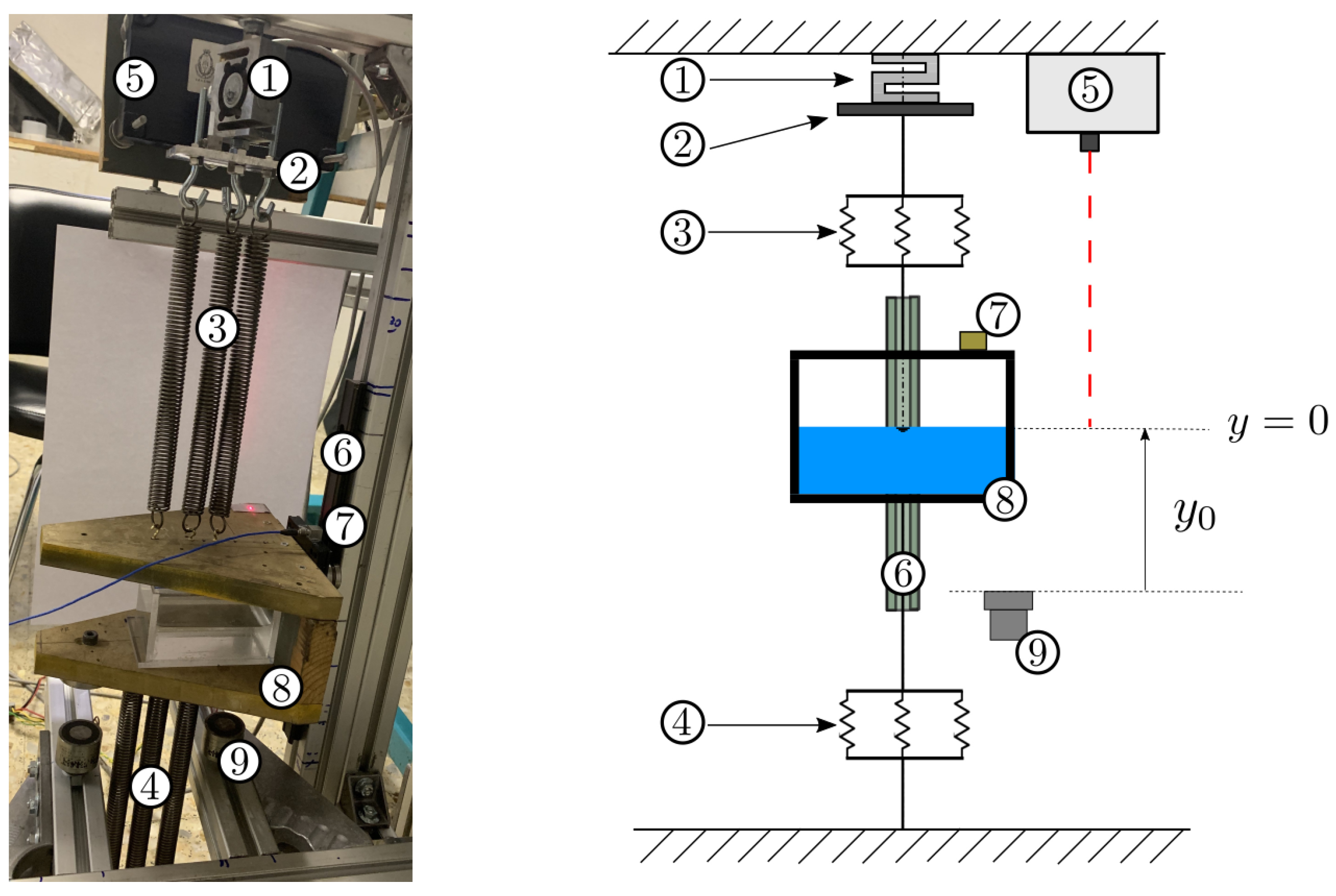


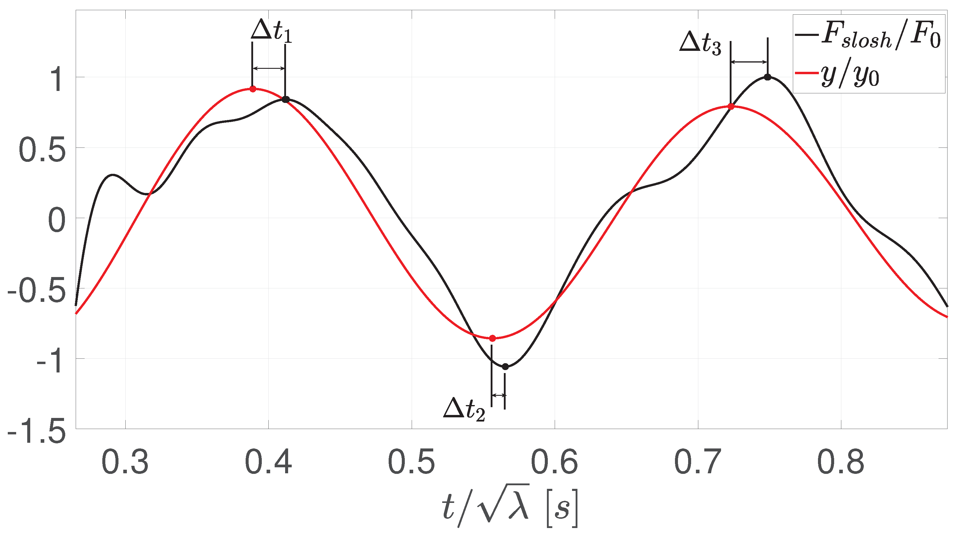
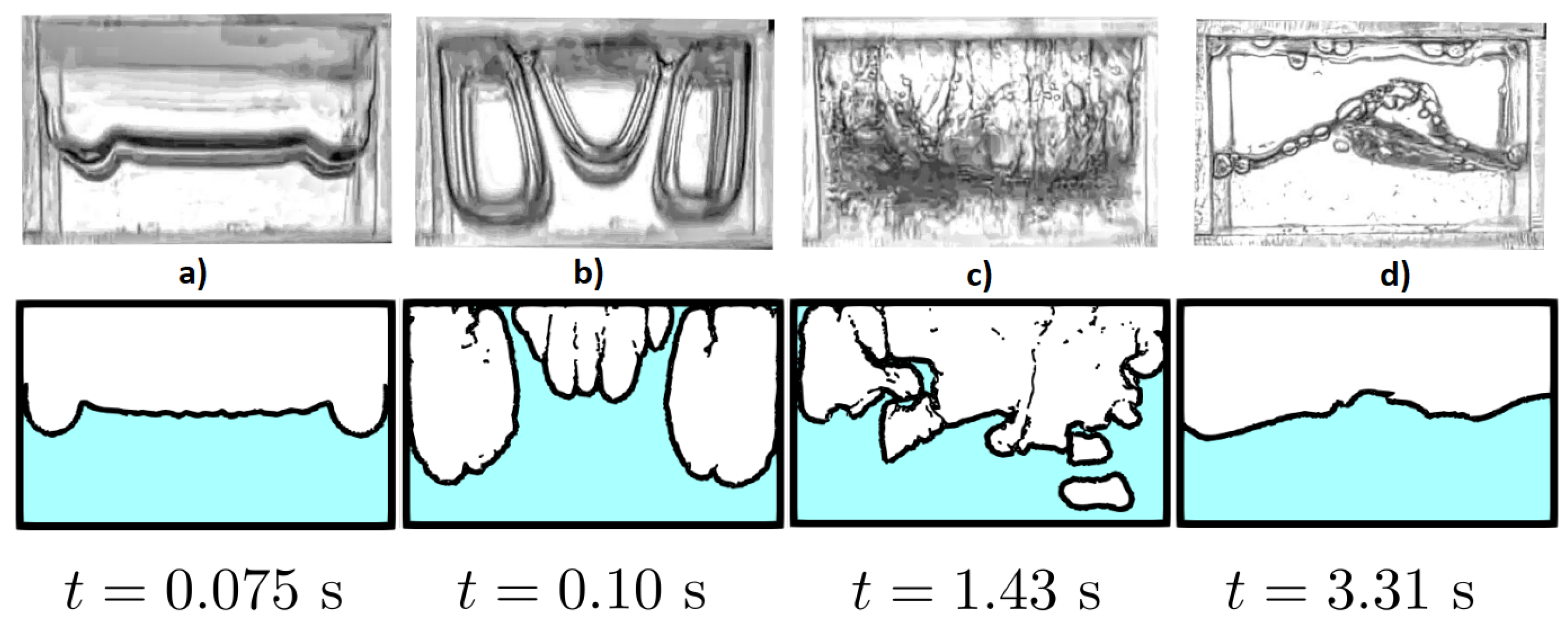
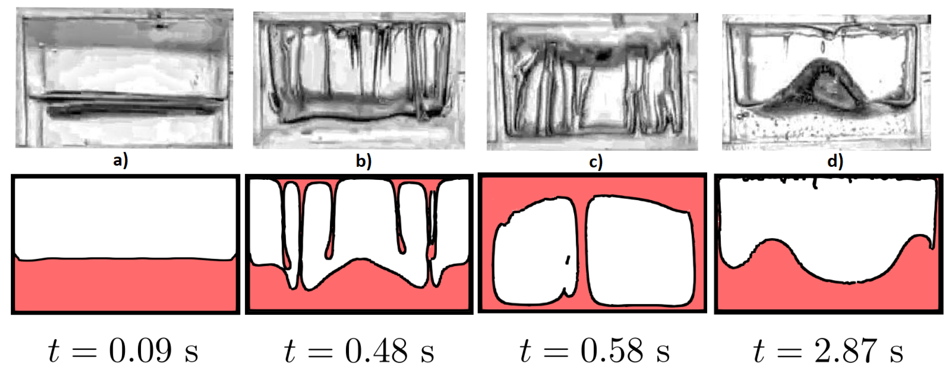
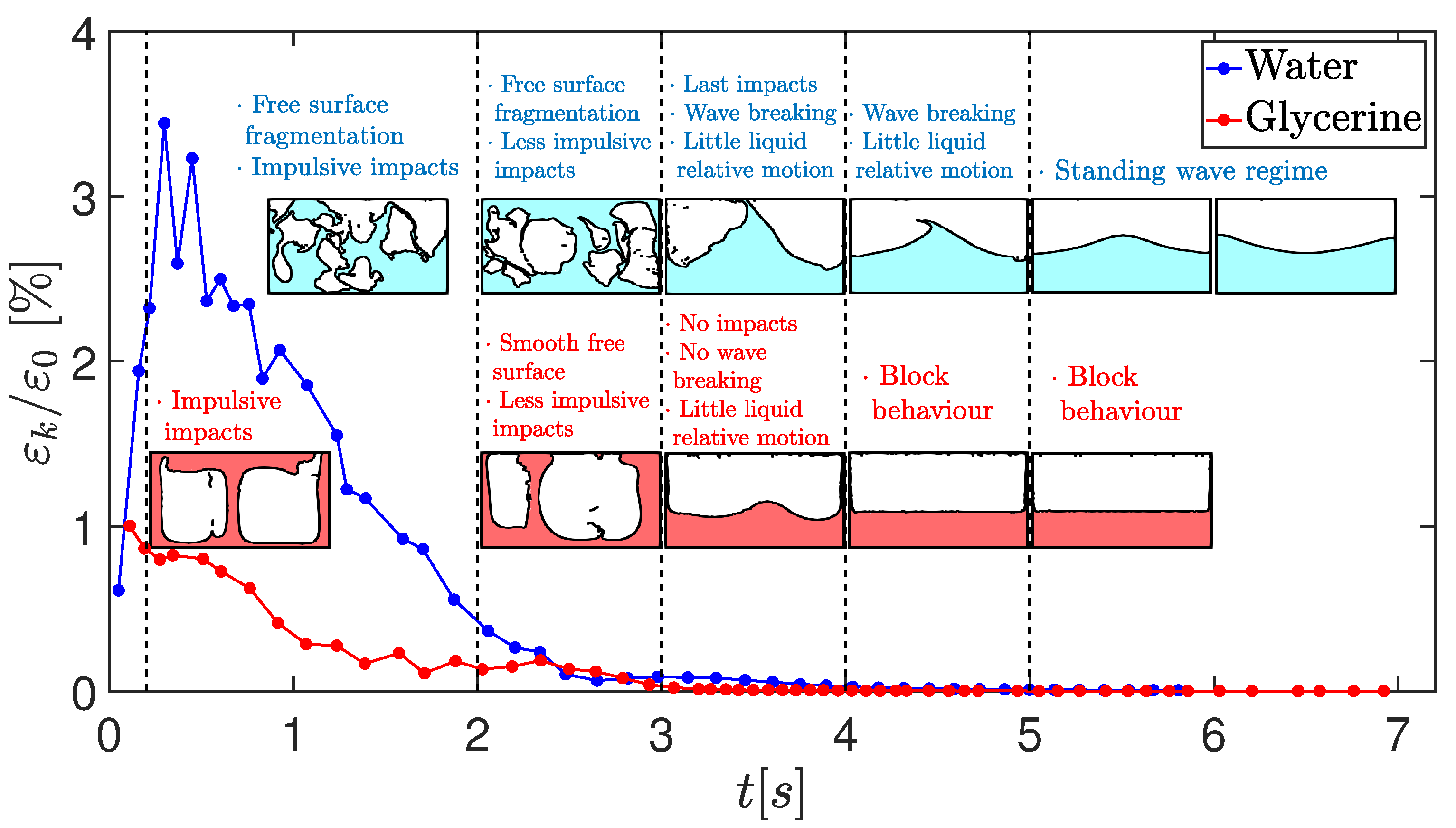
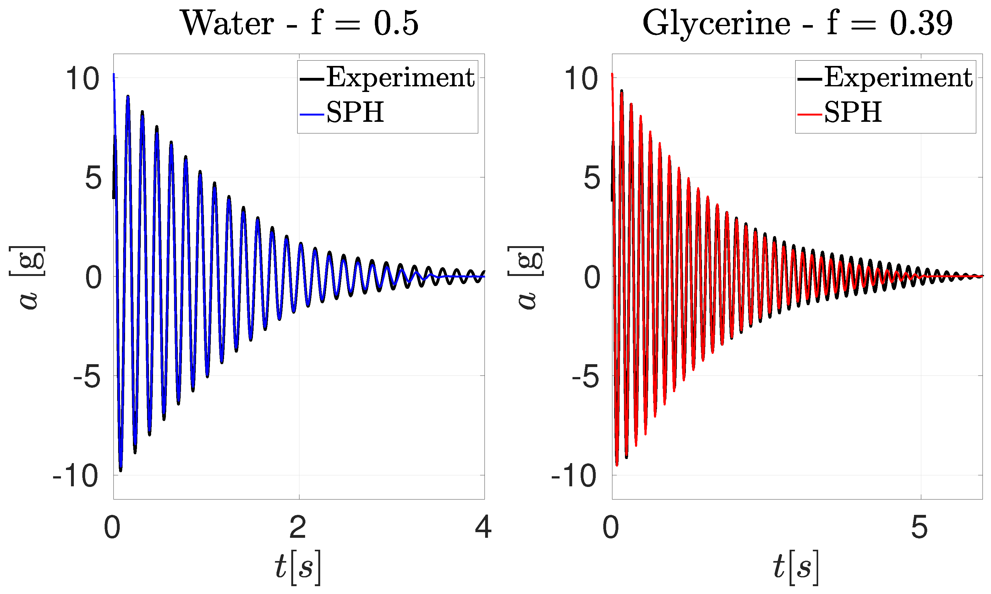
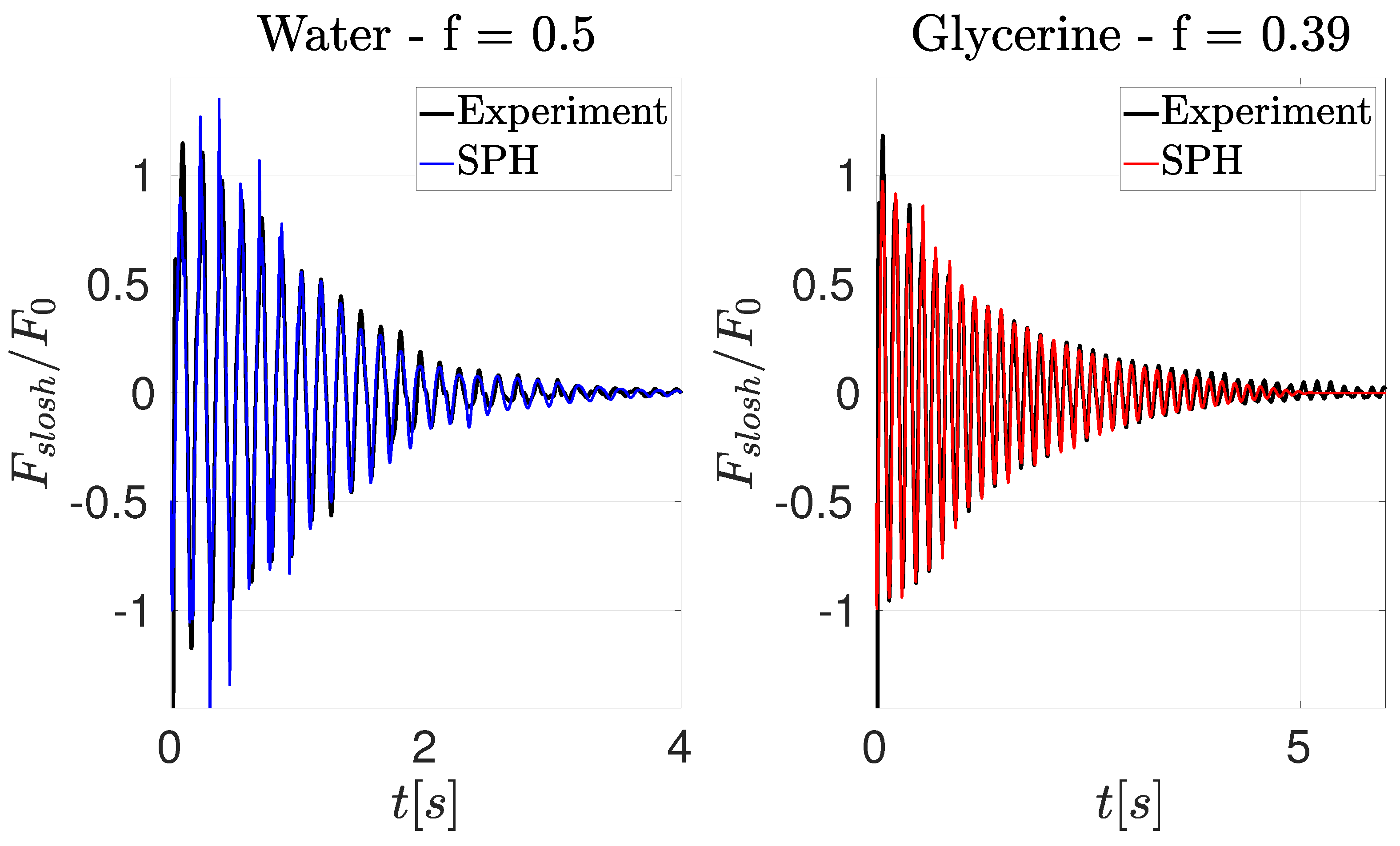


