Simulating Slosh Induced Damping, with Application to Aircraft Wing-like Structures

Abstract

The added damping generated by liquid sloshing in a tank has been utilized in a number of civil applications, including aviation, to reduce the vibration of the system. As part of a wider EU H2020 project called SLOWD (Sloshing Wing Dynamics), the presented study performed numerical simulations on the slosh-induced damping of liquid in tanks that were under free decay oscillations and embedded in an aircraft wing-like structure. A new open-source partitioned fluid–structure interaction software framework is presented and employed for the numerical simulations. Periodic sloshing waves and violent vertical fluid motions are observed in the study. These demonstrate the effects of slosh-induced damping under different excitation amplitudes of the structure and a varying number of baffled regions within the tank. Various sloshing patterns caused by different combinations of the excitation amplitude and compartment numbers lead to different induced dampings of the free decay motion. We observed a distinctly non-monotonic function on the slosh damping when the initial excitation amplitude is small (i.e., 0.25), with a 59% reduction when we increase the number of baffled compartments from one to four, and a 153% increase when moving from one to eight compartments. This is due to the change in the sloshing wave frequency, resulting in a significant change in the impact of the fluid between the tank ceiling and the wave crests. When the initial excitation amplitude is large (i.e., 1.0), there is no significant change in the slosh-induced damping when changing the number of compartments in the tank, for the range of parameters considered, due to the highly turbulent fluid motion. This work is expected to form the basis of further, more detailed studies within the context of the SLOWD project and its ever-expanding experimental data output.

1. Introduction

Liquid sloshing in a partially filled container is of significant interest in multiple disciplines. It is a non-linear and transient phenomenon that is challenging to simulate. The walls of the container will be subject to impact loads when liquid sloshing occurs. These loads can be significant when the natural frequency of the sloshing system and the excitation frequency are close and such large impulsive impact loads can result in damage on the structure of the container walls [1,2,3]. Alongside the issue of impact loading, liquid sloshing will, in general, provide added damping to the system. If considered correctly, this has the potential to be exploited in order to reduce the overall vibration of the system. The mechanics of the added damping and the energy dissipation changes, as well as relevant civil applications, are of widespread interest [4,5].

Studies specifically related to the mechanics of added damping generation and the associated energy dissipation of a sloshing tank have been reported in several articles. A series of experiments was carried out by Keulegan [6] in which they used rectangular basins to investigate the mechanics of the energy dissipation of standing sloshing waves. Dissipation of the waves was also observed and found to be due to the viscosity caused by surface tension. Another notable example can be found in Jiang et al. [7], where standing waves were investigated both experimentally and numerically. They observed dimpled crests when a steep wave appears, while the temporal symmetry of the resultant standing sloshing wave became broken due to energy dissipation. A follow-up study was performed in Jiang et al. [8], in which three recurrent modes of breaking waves were observed by increasing the forcing amplitude. The authors also found that energy dissipation was almost double when breaking waves occur.

One of the earliest civil applications of slosh-induced damping is the tuned sloshing damper (TSD), which aims to dampen the vibrations of a building. On-site measurements were carried out by Tamura et al. [9] to quantify the performance of the tuned sloshing-damper system for four tall buildings. Results showed that the TSD system can help a tall building to reduce half to one-third of the acceleration responses caused by strong winds by carefully selecting the water-mass ratio according to the total mass of the building. Ikeda and Nakagawa [10] performed both experimental and analytical investigations on the non-linear vibrations of a structure coupled with a sloshing water tank, targeting applications such as elevated water tanks or storage tanks for liquefied natural gas. The system was subjected to a sinusoidal excitation with a series of amplitudes. They found that the shapes of the resonance curves of the structure change with different water depths of the sloshing tank. The amplitude of the structure is very small when the system is close to the tuning frequency and under a small excitation amplitude (i.e., an amplitude equal to 0.205 N, 0.139 N and 0.152 N, respectively), while a complex oscillation motion occurs when the excitation amplitude is large (i.e., equal to 0.64 N). In similar work, Bouscasse et al. [11] considered a driven pendulum connected to a TSD to investigate its induced wave breaking and the associated energy dissipation generated by the shallow water sloshing of a TSD system. Large roll motions of up to 55º and subsequent complex flows occurred in this system and so a particle-based Lagrangian smoothed particle hydrodynamics (SPH) solver was employed to simulate the system in terms of its frequency behaviour in order to allow large deformation within the solution. For small excitation, low-amplitude travelling waves were observed. While for large excitation, violent fluid motions and breaking waves were observed. They also noted a significant change in the frequency response of the system with large excitation. As the second part of the same study, Bouscasse et al. [12] conducted experiments to measure systemic energy dissipation. By changing the liquid from a highly viscous liquid (glycerine), to a less viscous liquid (water), the oscillation amplitude of the pendulum-TSD system reduces. Here, water is clearly shown to counteract the effect of roll more quickly during the first several cycles, compared with glycerin.

The idea of slosh-induced damping has also attracted the attention of civil aviation. Merten and Stephenson [13] conducted experiments on the dynamic effects of a cantilever beam with a fuel-sloshing tank subject to sudden bending oscillations. They observed substantial damping induced by the sloshing tank that varies notably according to the filling level, the density of liquid, and the transient cycle number. Reese [14] experimentally studied the impact of a pylon-mounted tank with sloshing fluid on the flutter of a rigid wing supported by bending and torsional springs. Both frozen water and sloshing water were considered and slosh-induced damping was observed in the system with liquid water. Sewall [15] carried out analytical studies on wing models with an internal sloshing fuel tank under a bending-to-torsion frequency ratio that was close to one. Consistently, the highest flutter speeds were observed when the compartment emptying sequence proceeded from the front to the rear, due to the centre of mass of the system shifting.

The EU Horizon 2020 SLOWD (Sloshing Wing Dynamics) project aims to further investigate the physics of fuel sloshing in order to minimise aeroplane structural design loads and increase passenger comfort [16,17]. The project also aims to integrate new software workflows into key areas of industry to support the use of the results.

As a precursor to the SLOWD project, Titurus et al. [18] performed a number of liquid sloshing experiments at the Airbus Protospace Lab located in the United Kingdom. This utilised a scaled cantilever beam and attached water tank to study the impact of the liquid filling ratio on slosh-related structural damping. Complex behaviour with strong nonlinear phenomena was observed, both in terms of the fluid and the structure. The friction and nonlinear stiffness generated by the tank, even when dry, were found to have an impact on the dynamics of the cantilever beam, while the liquid sloshing phenomena when the tank contained fluid dominated the overall dynamics of the system. A filling level of 50% was found to provide the strongest damping effect. With the same experimental setup, Gambioli et al. [19] studied the impacts of dry-roof/drop-impact-roof and different liquids, i.e., water and kerosene, on the behaviour of the sloshing tank-beam system. They found that the response of the system during the initial oscillation is dominated by an apparent Rayleigh–Taylor instability at the free surface. The system with both the dry-roof and drop-impact-roof showed similar responses in terms of the time histories from accelerometer and strain gauge data. As well as the experiments on the cantilever beam, Martinez-Carrascal and González-Gutiérrez [20], Constantin et al. [5] and Constantin et al. [21] carried out experiments on the sloshing-induced damping of a harmonically vertically excited sloshing tank.

The present study employs a CFD approach based on finite volumes and using the volume of fluid (VoF) method to capture the free surface. In Ilangakoon et al. [22], a VoF-based curvature calculation method was proposed and validated for the modelling of surface tension in highly dynamic free-surface problems. A novel sweep-line algorithm was employed based on volume conservation and representing the free surface using a piecewise-linear representation. A number of test cases were carried out and showed second- and fourth-order accuracy, depending on the case. In Oomar et al. [23], the Harten–Lax–van Leer contact solver was then combined with a VoF-based compressive interface capturing scheme for arbitrary meshes. Several benchmark cases were carried out that showed the method provides accurate and reliable results and is able to improve the accuracy of free-surface capturing. Within the SLOWD project itself, VoF-based solvers have been successfully employed for the simulation of violent slosh-induced energy dissipation [24], slosh loads [25] and also coupled with a structural solver on fluid–structure-interaction-based slosh damping simulations [26].

The SLOWD project also considers other simulation methods, including the use of an SPH model: Calderon-Sanchez et al. [27] investigated the added damping of the spring-mass-based vertical sloshing tank, as well as the creation of reduced order models [28,29,30].

As an integral part of the overall SLOWD project, the present study simulates the slosh-induced damping of partially filled water tanks on an aircraft-wing-like structure under free decay oscillations, employing open-source software. It involves the development of a new, fully coupled, fluid–structure interaction solution for the modelling of the interaction between the sloshing tank and the structure. In these results, the impact of the excitation amplitude of the structure and the number of baffled regions within the sloshing tank are investigated. Results are taken over the first ten free decay oscillation cycles and the resultant slosh-induced damping is explored. The simulations provide numerical insight into the damping behaviour of the sloshing system, as well as the corresponding slosh patterns in different excitation conditions and using different compartment numbers. The results obtained compare favourably with independent experimental results also generated within the SLOWD project and will be useful to the community by providing an in-depth understanding of the slosh-induced damping in the aviation field, with outputs being used directly as guidance for the design of next-generation wing technology.

This paper is organised as follows: the problem description and numerical setup used are presented in Section 2 and Section 3, results and discussions on free decay of an oscillated aircraft-wing-like structure including sloshing tank simulation are presented in Section 4 and a summary of conclusions and future works of this study is presented in Section 5.

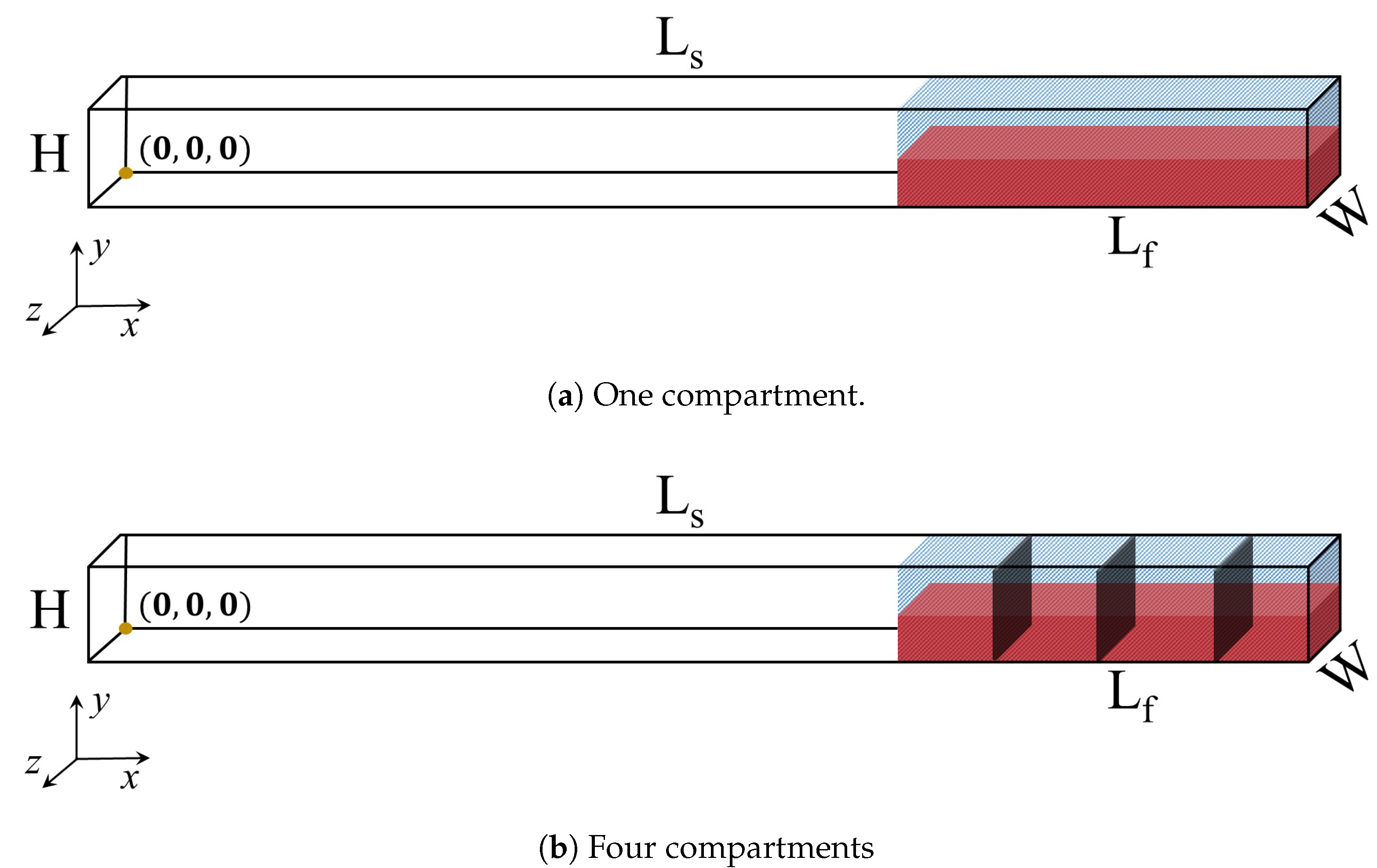
2. Problem Description

In this study, a simplified aircraft-wing-like structure is used based on a series of experiments that were recently performed at the Airbus Protospace Lab in Filton (Bristol, UK) to explore the interaction between the sloshing tank and the motion of a beam with moderate initial deflections [18,19]. The simplified system consists of a hollow cantilevered steel beam with a sloshing water tank attached on top. The length, height and width of the beam are $L_s=12$ m, $H=0.3$ m and $W=0.55$ m along the x-, y- and z-axes, respectively. The thickness of the walls of the beam is $0.22H$. The dimensions of the beam are determined based on a full-scale single-aisle airliner wing and the first bending frequency of the elastic beam is approximately 2 Hz, with the period $T=0.5$ s, to match the natural frequency of the wing [19]. In the present simulation, an idealised beam is used, in which the damping matrix of the elastic beam is set to zero and the gravitational force on the beam is ignored. This eliminates any influence from both the mechanical damping and the weight of the beam on the final result. The beam is made of steel, with a density, Young’s modulus and Poisson’s ratio of 8050 kg/m${}^3$, $2\times {10}^{11}$ Pa and $0.3$, respectively. The elastic beam is fixed at one end to represent the connection between the aircraft wing and the fuselage and free at the other end. The fuel tank inside the wing of the aircraft, where the sloshing phenomena occur, is also idealised as a hexahedral water tank in this study. The water tank is embedded inside the hollow section of the beam and is mounted close to the free end to represent the fuel tank of the aircraft, as proposed by Titurus et al. [18] and Gambioli et al. [19].

The tank has the same height and width as the beam, while the length is $L_f=3.5$ m. The water tank is filled to $50\%$ throughout this study. Gravitational acceleration is applied to the water tank in the negative y-direction. The density and dynamic viscosity of the water are 1000 kg/m${}^3$ and 0.001 N · s/m${}^2$, respectively, and the surface tension of the fluid is set to $0.0728$ N/m. The mass ratio between the fully loaded fluid tank and the beam is $0.07$, again to match the working conditions of a civil aircraft with reserve fuel [18].

The present study assumes an initial meniscus for the fluid, as in Figure 14 of Constantin et al. [5], in order to replicate the wetting effect of water on the tank wall. One objective of this study is to investigate how slosh-induced damping is affected by the number of compartments of the water tank. Four designs are considered in this study, one, two, four and eight compartments. Examples are shown in Figure 1a (one compartment) and Figure 1b (four compartments). Internal baffles are used to separate the water tank into the separate compartments that block mass and momentum exchange between them.

An external load is uniformly applied to the upper x–z surface of the beam–tank system along the negative y-axis direction between $-0.5$ s and 0 s. The external load is applied in the y-axis direction because atmospheric turbulence typically excites an aircraft wing along this axis and direction during cruise flight conditions. The y-axis external load is designed to mimic the effect of the atmospheric turbulence excitation. Timing starts once the external load is removed. After 0 s, the beam–tank system is excited by the external load and subject to free decay oscillation motion. As reported by Constantin et al. [5], the largest damping and the highly turbulent fluid motion takes place within the first $1.5$ s (around 15 oscillation cycles) of the transition, with this being the most crucial to use for reducing aircraft gust loads. Similarly, a large damping and turbulent fluid motion can be observed in the first 1 s (around 6 oscillation cycles) of the free-decay motion of the sloshing tank, Titurus et al. [18]. It is clear that the response envelopes, damping behaviour, and slosh pattern of the first several cycles (around 6 to 15 oscillation cycles) are significantly different from the subsequent cycles, according to [5,18]. The scope of this study is to provide numerical insights into this region to understand its damping behaviour and corresponding slosh patterns.

We focus on the behaviour and slosh-damping profile in the first 10 cycles of the free-decay oscillation in this study to take into account the results of different experiments, as well as computational resources. The magnitude of the external load was carefully selected to achieve the desired excitation amplitude of the beam–tank system, as suggested by experiments in the literature [18,19]. More specifically, we define $D_{amp}$ as the initial excitation amplitude, which is the oscillation amplitude of the beam–tank system within the first cycle. The non-dimensional version of the initial excitation amplitude, $D_i$, is defined as

$$D_i=\frac{D_{amp}}{H}.$$

(1)

Three values of the non-dimensional initial excitation amplitude are adopted in this study, which are $1.0$, $0.5$ and $0.25$; these match the parameter range of the experiments by Titurus et al. [18] and Gambioli et al. [19]. In each oscillation cycle, the tip of the beam starts from the lowest position and spends half of the cycle for its upstroke.

3. Numerical Methodology

3.1. The Simulation Framework for Fluid-Structure Interaction

To simulate the free decay of an oscillating aircraft-wing-like structure with a sloshing tank, a newly developed and open-source multiphase FSI framework, ParaSiF [31,32] is employed. This has undergone extensive verification for problems such as the one considered herein, Liu et al. [31,33]. Figure 2 shows a flowchart of the algorithmic design of the framework, which follows a partitioned approach, in which a multiphase computational fluid dynamics (CFD) solver is coupled with a computational structural mechanics (CSM) solver through a general purpose coupling library. In the present study, the CFD solver interFSIFoam is built using the OpenFOAM [34] suite, the CSM solver using the FEniCS v2019.1.0 [35] framework and the Multiscale Universal Interface (MUI) [36] is used as the coupling library.

3.1.1. Multiphase Fluid Solver

The continuity equation and the momentum equation over an arbitrary moving volume of the developed multiphase fluid solver interFSIFoam [31] read as [37,38]

$$\nabla ·\mathit{U}=0,$$

(2)

$$\frac{\partial {\rho }_f\mathit{U}}{\partial t}+\nabla ·[\mathit{U}·{\rho }_f(\mathit{U}-{\mathit{U}}_{\mathit{s}})]=-\nabla p+\nabla ·({\mu }_f\nabla \mathit{U})+{\mathit{s}}_{\varphi }$$

(3)

where $\mathit{U}$ is the velocity of fluid, ${\rho }_f$ is the density of fluid, t is the time, ${\mathit{U}}_{\mathit{s}}$ is the grid velocity, ${\mu }_f$ is the fluid dynamic viscosity, p is the pressure of fluid and ${\mathit{s}}_{\varphi }$ is a source term combining both surface tension and gravity. An arbitrary Lagrangian–Eulerian (ALE) formulation based on the space conservation law is used to close the momentum equation [38]. The free-surface of multiphase flow is captured by the VoF method [39] and is constructed with the multidimensional universal limiter for the explicit solution (MULES) scheme. This study employs an artificial interface compressibility scheme [40] and is set conservatively with the value of OpenFOAM keyword cAlpha to the widely adopted value of unity [31]. The interFSIFoam solver also undertakes functions of exchange data (such as fluid forces and structural displacement) with the structure solver through the MUI coupling library and conducting sub-iterations at each time step for a two-way implicit FSI coupling.

3.1.2. Elastic Structural Solver

The in-house elastic structural solver is based on the finite element method and is developed using the FEniCS library [35]. Assuming body-fitted coordinates, the generalized n-DOF (degrees of freedom) harmonic oscillator (GHO) equation with mass matrix, $\mathit{M}$, damping matrix, $\mathit{C}$, stiffness matrix, $\mathit{K}$, and external loading, $\mathit{F}$, are expressed as

$$\mathit{M}\frac{{\partial }^2\mathit{d}}{\partial t^2}+\mathit{C}\frac{\partial \mathit{d}}{\partial t}+\mathit{Kd}=\mathit{F}\left(t\right)$$

(4)

where $\mathit{d}$ is the deformation of the structure. The damping matrix is assumed zero to represent an idealised mechanical damping-free structure.

As is typical for this type of problem, a second-order generalised-$\alpha$ method is used for time stepping [41,42,43]. In this study, the maximum tip vertical displacement of the structure is no larger than 2.5% of its total span. It is, therefore, within a geometrically linear regime at all times and a generalised n-DOF harmonic oscillator equation is able to handle this problem with sufficient accuracy.

3.1.3. Fluid–Structure Interaction

The CFD and CSM solvers are fully coupled through the MUI coupling library. The kinematic and dynamic conditions at the fluid structure interface read as [37,44]:

$${\mathit{d}}_{\mathit{s}}={\mathit{d}}_{\mathit{f}}$$

(5)

$${\sigma }_s·\mathit{n}={\mathit{t}}_{\mathit{f}}$$

(6)

where ${\mathit{d}}_{\mathit{s}}$ and ${\mathit{d}}_{\mathit{f}}$ are the interface displacement in the structure and fluid domains, ${\sigma }_s$ is the stress tensor and ${\mathit{t}}_{\mathit{f}}$ is the traction at the interface. The MUI built-in radial basis function (RBF) spatial interpolation method is employed to ensure the conservation of the forces acting on the interface between the two domains with non-conformal meshes [45,46]. The present study employs the Aitken’s fixed point iteration method with several sub-iterations within each time step to achieve a tight coupling. Both the CFD solver and the CSM solver always have the same time-step size, which is set by ensuring Courant–Friedrichs–Lewy (CFL) numbers in different solvers are all smaller than their respective criteria based on their numerical methods.

Further details of the workflow of the open-source FSI simulation framework can be found in Liu et al. [31,47,48]. The open-source framework has been extensively validated, showing good accuracy for the simulation of multiphase FSI problems [31,47,48].

3.2. Numerical Setup

In this study, the behaviour of the cantilever beam and the sloshing inside the tank are modelled by the CSM and CFD parts of the multiphase FSI framework independently. A set of meshes are, therefore, needed for both domains. A quadratic Lagrange tetrahedral-based mesh is generated for the structural domain [49], while a hexahedral-based structured mesh is generated for the fluid domain. Following a grid convergence study, 12 million hexahedral cells and 12.7 thousand DOF were adopted for the CFD and CSM meshes, respectively. It was found that using double the number of cells/DOF produced values within a few percent of the coarser solutions. The meshes used for the simulations of this study are shown in Figure 3. The time-step size and the OpenFOAM keyword nAlphaSubCycles of the simulation was carefully chosen per case to ensure the Courant number and the interface Courant number per VoF step in the fluid domain all remain below $0.5$.

The numerical setup for the simulations within this study follow that of the validation and the demonstrative cases in Liu et al. [31,33], except for the turbulence model, where the $k-\omega SST$ is used according to Tahmasebi et al. [50] and Huang et al. [51]. A no-slip boundary condition was employed for all six boundaries of the fluid domain. For the structural domain, a fixed boundary was set for the $x=0$ m plane for the cantilever beam, while other boundaries were set as free, with zero traction by default. The Aitken’s method was employed to achieve a tight coupling between the fluid and structural domains.

4. Results and Discussion

The main objective of this study is to carry out investigations into how slosh-induced damping is affected by the excitation amplitude, and number of compartments, of an aircraft-wing-like structure over the first ten free-decay oscillation cycles. In this study, gravity is applied to the sloshing tank and the fluid inside but not the structural domain. The amplitude of the idealised structure remains constant without any damping if the tank is not present. Any damping in terms of the tip vertical displacement of the structure can be entirely attributed to the sloshing tank, i.e., slosh-induced damping. This is an effective way to carry out a decoupled analysis that highlights damping effects of interest while excluding unwanted physical factors but is challenging experimentally.

4.1. The Slosh-Induced Damping Ratio of an Oscillated Aircraft-Wing-like Structure

As per Section 2, an idealised cantilever beam with no structural damping is employed as part of this decoupled analysis in order to highlight only the damping induced by the attached sloshing tank. For a beam–tank system with frozen water, the tip displacement of the system under a free-decay oscillation will maintain the same amplitude from cycle to cycle (with the shape of its time history being a basic sinusoidal wave), as there is no damping source involved in the system. The time history of the tip displacement of the system can be expressed as a damped sinusoidal function as

$$D=D_{amp}·e^{(-\lambda t)}cos(2\pi \frac{t}{T}-\varphi ),$$

(7)

where D is the instantaneous tip displacement of the system along the y-axis direction, e is Euler’s number, $\lambda$ is the decay rate, and $\varphi$ is the phase angle at $t=0$. The damping ratio of the tip displacement is denoted as $\zeta$ and is defined as

$$\zeta =\frac{\lambda }{\sqrt{{\lambda }^2+{\left(\frac{2\pi }{T}\right)}^2}}.$$

(8)

The tip displacement damping ratio is a non-dimensional parameter to quantify the decay rate of the free oscillation of the beam–tank system relative to its natural frequency. We note that $\zeta =0$ for the frozen water case, as would be theoretical expected, and confirm the levels of numerical dissipation are not adversely affecting our results. Meanwhile, the beam–tank system with sloshing water is expected to have a non-zero value for the damping ratio. In this study, the ratio of a case is obtained by finding the best fit of the time history data of the vertical tip displacement of the system during $t/T=0$ and $t/T=10$, according to the damped sinusoidal function.

The global view of the damping ratio of the free decay beam–tank system with both sloshing water and frozen water as a function of the number of compartments, $N_c$, and within the parameter range of this study, is shown in Figure 4. For compartment number $N_c=1$ (i.e., with no baffles placed inside the tank), the slosh-induced damping of $D_i=1.0$ is close to that of $D_i=0.5$, with a difference of approximately $2\%$. In contrast, the slosh-induced damping of $D_i=0.25$ is much smaller than the other two cases, at around $48\%$ of that with $D_i=1.0$. By including baffles into the tank and increasing the compartment number from one to two, four and eight, the slosh-induced damping with $D_i=1.0$ does not appear to change significantly. For $D_i=0.5$, the slosh-induced damping with two compartments is quite close to that with one compartment. Continuing to increase the compartment number to four and eight, the slosh-induced damping with $D_i=0.5$ increased by $18\%$ and $24\%$, respectively. The damping of $D_i=0.25$ with different compartment numbers shows a distinctly non-monotonic function, with significant variation within the parameter range of this study. As the number of compartments is increased from one to four, the slosh-induced damping dropped by approximately $59\%$. As the number of compartments is increased to eight, the slosh-induced damping also increases by $153\%$ compared to with one compartment.

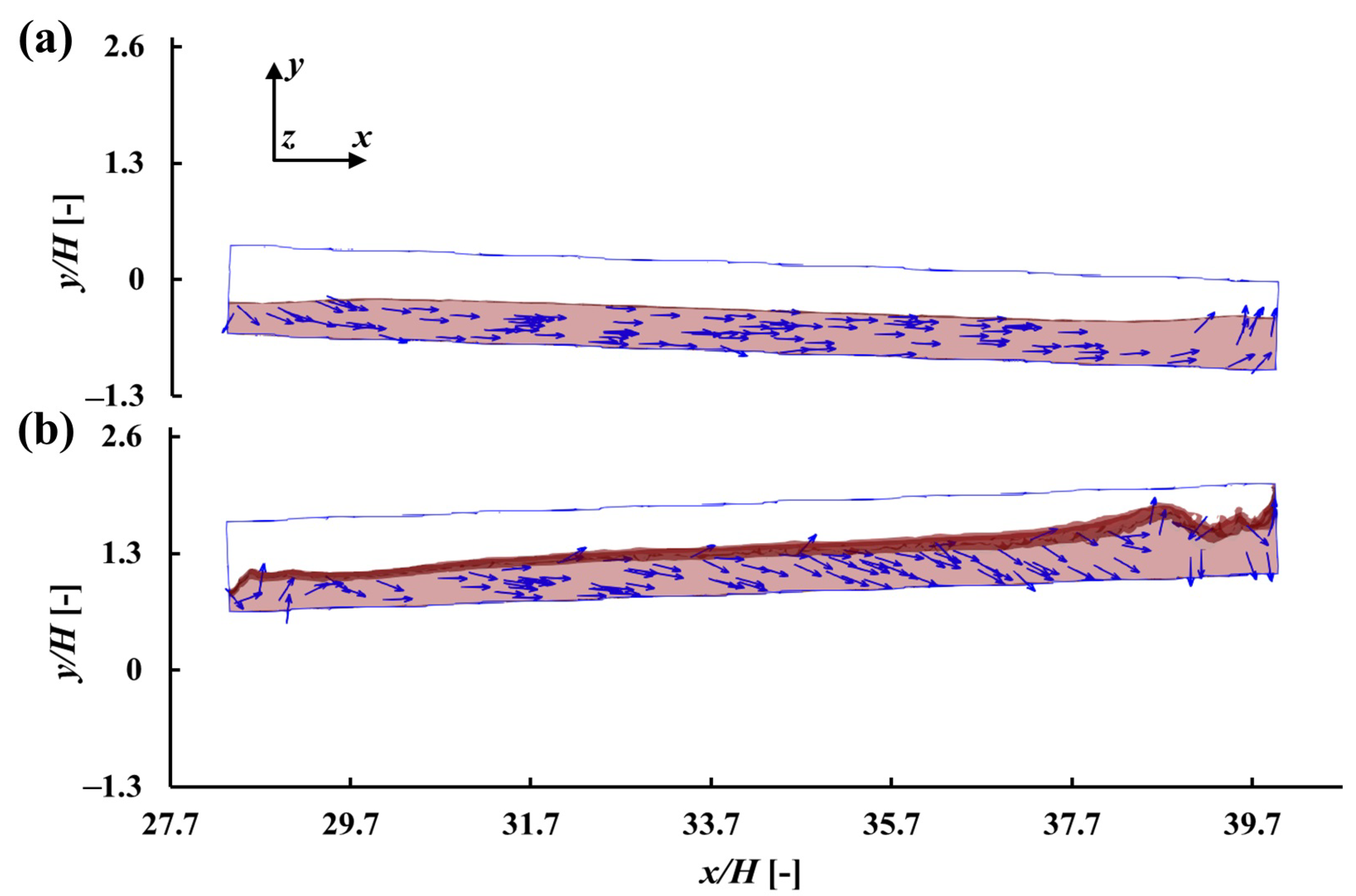
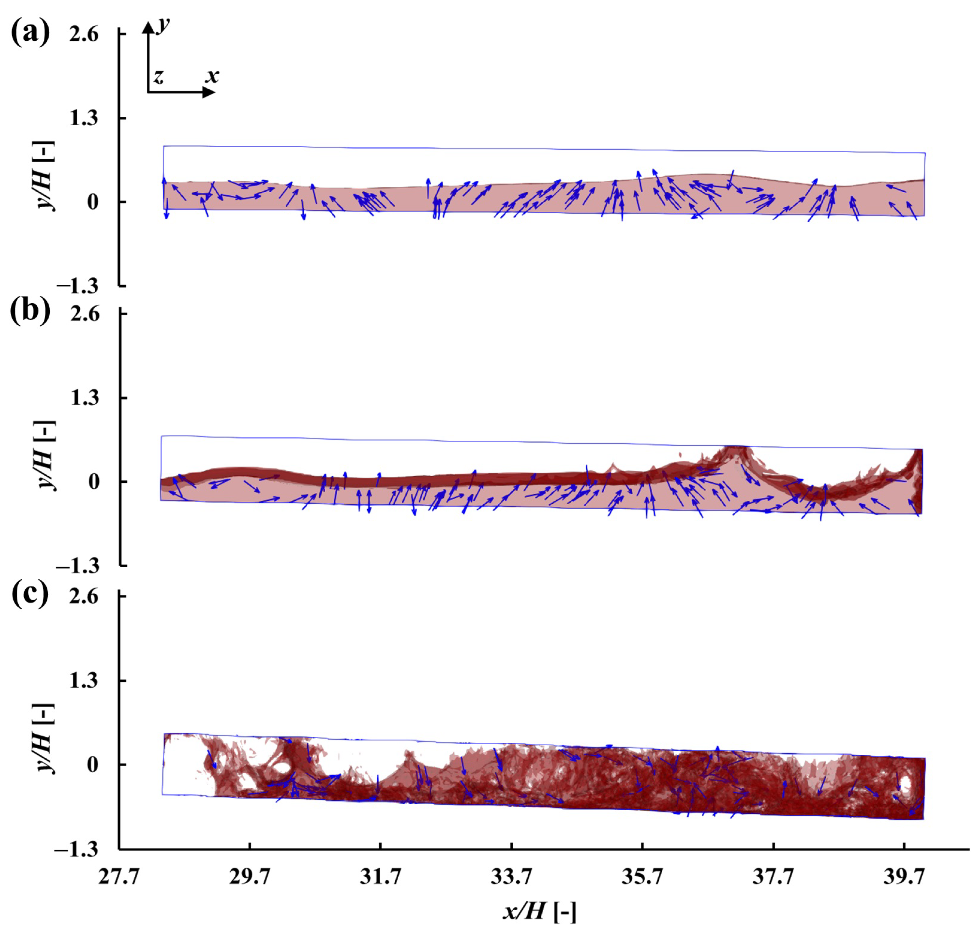
4.2. Impact of Initial Excitation Displacement with One Compartment

The impact of the initial excitation displacement on the slosh-induced damping ratio with no baffles was considered. The instantaneous non-dimensional tip vertical displacement of the system, as well as the instantaneous non-dimensional vertical fluid force of the water tank, over ten oscillations and different initial excitation amplitudes, are shown in Figure 5a,b. These show the vertical fluid force of the water tank, $F_y$, non-dimensionalised according to the gravitational force of the water tank, $F_g$. The fluid force follows the positive upwards y-direction. The tip vertical displacement and vertical fluid force of the beam–tank system with frozen water are also shown in Figure 5a,b. Compared with the system with frozen water, the tip vertical displacement of the beam–tank system with sloshing water shows clear damped sinusoidal curves, as in Figure 5a. The vertical fluid force shows similar spike curves but different amplitudes for different $D_i$. In order to cross compare the tip vertical displacement and vertical fluid force among different initial excitation amplitudes, we normalised the non-dimensional tip vertical displacement and the non-dimensional vertical fluid force by the value of the initial excitation amplitude, as shown in Figure 5c,d.

There are two key approaches for investigating the beam–tank model. The first approach is to establish a non-inertial frame of reference based on the tank’s body-fitted coordinates. Under this approach, the focus is the fluid and, therefore, we can investigate the cause and mechanism of the sloshing patterns under different conditions. The forces acting on the water consist of the gravitational, inertial and forces due to the sloshing motion. As both the inertial force and the sloshing force are functions of time, the total force acting on the water is also a function of time. The second approach is to establish an inertial frame of reference based on global coordinates. The focus then is the whole system instead of the fluid. This second approach is a convenient way to investigate how different sloshing patterns affect the free-decay motion of the system.

Using this approach, we are interested in the forces acting on the beam by the sloshing water. There is no inertial force to be considered as the observer is in the inertial frame of reference. The presented study follows this second method in order to investigate the impact on the free decay motion of the system of the sloshing water. The vertical fluid forces shown in Figure 5b,d are those acting on the beam by the fluid.

The vertical motion (along y-axes direction) of the tip of the beam–tank system can be qualitatively analogized with a vertical 1-DOF mass-spring-damper model with gravity. If there is no tank in the hollow beam, the vertical motion of its tip is similar to a hinged spring as an idealised beam is used in this study. If a tank with frozen water is introduced into the hollow beam then it is equivalent to hanging a mass block on the vertical spring and letting it naturally oscillate. There is no damping involved in the system. The only force acting on the beam (or spring) is the constant gravitational force of the frozen water (or the block). The impact of the gravitational force is to change the equilibrium position of the system, i.e., an offset in both the tip vertical displacement and the vertical fluid force. Finally, if a sloshing tank is introduced, this is then equivalent to a sloshing mass block hanging from the spring, and there will be sloshing forces acting on the beam (or spring) on top of the gravitational force of the water. This study will pay particular attention to the impact of the sloshing forces on the oscillation motion of the system.

From the third oscillation cycle, the effect of slosh-induced damping is evident for all initial excitation amplitudes, as can be seen in Figure 5c. Meanwhile, during the last five oscillation cycles, the amplitude of the tip vertical displacement for $D_i=0.25$ is larger than that of $D_i=1.0$ and $D_i=0.5$. This indicates that the slosh-induced damping for $D_i=0.25$ is smaller than that of $D_i=1.0$ and $D_i=0.5$, which is the same conclusion seen in Figure 4.

As mentioned in Section 2, each oscillation cycle of the beam-tank system starts from its tip, located at the lowest position for its upstroke in the positive y-direction. The vertical fluid force reaches its minimum value (i.e., the maximum negative value) at the proximity of the beginning of each oscillation cycle, where the bulk of the water pushes against the floor of the tank. The fluid force reaches the maximum value at around the middle of each cycle as the tip of the system reaches the highest position, where the bulk of fluid has been accelerated in the positive y-direction and sloshing waves are formed. The spikes of the vertical fluid force are distinct from cycle to cycle, as shown in Figure 5d. This is partially due to the nature of the problem that the sloshing motion of the fluid is subject to rapid development during the first ten oscillations and also due to the non-linear nature of the sloshing regime within this study (reported in Constantin et al. [21]). It can be seen in Figure 5d that the vertical fluid force of the sloshing tank with $D_i=0.25$ is smaller than that of the other two initial excitation amplitudes at the beginning of each oscillation cycle.

We further investigated the fluid domain for a better understanding of the observations in Figure 4 and Figure 5d. Through this, it was found that the shape of the sloshing waveform in the first half cycle is similar from case to case with one compartment within the parameter range of this study. An example can be seen in Figure 6, which shows the snapshots of the water phase within the sloshing tank with $D_i=1.0$ and $N_c=1$ at the beginning and the half of the first oscillation. The water phase is shown as transparent red with dark red representing the free surface and pink representing the bulk of liquid without free surface. Blue arrows show the general direction of motion of the sloshing water in the global reference frame. It can be seen that, at the very beginning of free decay cycles (i.e., $t/T=0$), the tip of the tank is located at the lowest position due to the external force, and is about to be accelerated towards the equilibrium position by the elasticity of the beam. The water inside the tank flows along the slope to the front due to gravity. The water starts to build up in the front of the tank. At the end of the first upstroke (i.e., $t/T=0.5$), initial slosh-induced waves start to form in the front and rear of the tank. There is no contact with the ceiling of the tank by the sloshing wave for all simulation cases within the parameter range of this study. It is noticed that the free surface is not visible at $t/T=0$ but can be seen clearly at $t/T=0.5$. The reason for this behaviour is mainly due to the $3-D$ shape of the slosh pattern. More specifically, at $t/T=0$, the slosh pattern has not yet developed and the elevation of the free surface along the lateral direction has the same value, while at $t/T=0.5$, the slosh pattern has started to develop and the elevation of the free surface along the lateral direction is no longer equal. This is consistent with reported experimental results [5,18]. In addition however, the present study applies a meniscus to the initial starting conditions of the fluid simulation in order to replicate the wetting effect of water on the tank wall before release. This perturbation causes the lateral motion of the water and contributes to creating a realistic $3-D$ slosh pattern.

From the down stroke of the first cycle onwards (i.e., $t/T>0.5$), the system with different initial excitation amplitudes begins to show different sloshing patterns in the water tank. A significant difference can be observed among different initial excitation amplitude cases from the third oscillation. Figure 7 and Figure 8 show snapshots for the sloshing tank of three different initial excitation amplitudes with one compartment at $t/T=2.0$ and $t/T=2.5$. It can be seen from Figure 7a and Figure 8a that the sloshing pattern for $D_i=0.25$ is dominated by gentle sloshing waves without any contact with the ceiling of the tank during the third cycle. The sloshing in $D_i=0.5$ is dominated by the same model pattern as in $D_i=0.25$, but due to the larger oscillation amplitude, the wave amplitude is larger than that of $D_i=0.25$ and the crest of the waves show impacts with the tank ceiling. Damping due to impact on the ceiling/floor of the tank is discussed in Constantin et al. [5] and Constantin et al. [21].

When the water impacts the ceiling of the tank, the resultant splash then falls back and impacts the floor. These ceiling and floor impacts introduce significant impact-driven turbulence and affects the fluid force acting on the tank wall. At $t/T=2.0$, there are three wave crests for both the $D_i=0.25$ and $D_i=0.5$ cases. The general direction of the motion of the water is from the crest of the wave towards the wave trough as shown in Figure 7, i.e., these are falling waves. When the system finishes its upstroke and reaches the highest position, crests and troughs alternate, as shown in Figure 8.

It can be seen that the amplitude of the wave crests in the front of the tank are larger than those in the rear. This is expected behaviour as the oscillation amplitude in the front of the tank is greater than that in the rear. For $D_i=1.0$, no sloshing modal pattern can be discerned. In this case, the sloshing is dominated by the turbulent vertical motion entirely. Strong impacts between the water and the top/bottom wall of the tank can be observed for both the beginning and the middle of the third oscillation cycle.

In Figure 9, the vertical fluid force during the third oscillation cycle is represented by the normalised force-velocity diagram, where the time parameter is eliminated. Similar to the vertical fluid force, the normalised tip oscillation velocity, $\delta DT/\delta tH{D}_i$, follows the positive upwards y-direction. The two grey solid lines ($F_y/F_g{D}_i=0$ and $\delta DT/\delta tH{D}_i=0$) divide the normalised force–velocity diagram into four quadrants. In the second and the fourth quadrants, the vertical fluid force and the tip oscillation velocity are in the opposite sign, which causes the vertical fluid force to decrease the momentum and increase the damping of the free decay in the system. In the first and the third quadrants, the fluid force and the tip oscillation velocity are in the same sign, so the fluid force increases the momentum and decreases damping. In each cycle, the normalised force–velocity loop starts from point A (the subscript label denotes the $D_i$ value), follows the green dotted arrow towards point B for its upstroke, and follows the other half of the loop to go back to point A with its down stroke. For the third cycle, the sloshing tank with $D_i=1.0$ has a larger fluid force in the second and the fourth quadrants, but a smaller fluid force in the first and third quadrants compared with that of $D_i=0.25$, this can be attributed to the impact of the violent fluid motion between the top and bottom of the tank. The normalised force–velocity loop for $D_i=0.5$ is quite close to that of the $D_i=0.25$ in the first, the second and the fourth quadrants. While the normalised force–velocity loop for $D_i=0.5$ in the third quadrants is close to that of $D_i=1.0$, which is due to the impact between the wave crest and the tank ceiling.

As time progresses, the water inside the tank is excited more by the oscillating beam, with the amplitude of the wave crests increasing. Figure 10 and Figure 11 show snapshots for the sloshing tank of three different initial excitation amplitudes with one compartment at $t/T=7.0$ and $t/T=8.0$, respectively. For $D_i=0.25$, we can observe impacts between the wave crests and the tank ceiling at both $t/T=7.0$ and $t/T=8.0$. The location of the wave crests is observed to move from cycle to cycle. This phenomenon is caused by the instability and non-linear behaviour of the sloshing and has also been observed by experiments in the literature [21]. In $D_i=0.5$, the sloshing in the front half of the tank is characterised by violent vertical impacting motion, while in the rear half the shape of the waveform with wave falling motion can still be observed. In $D_i=1.0$, the sloshing is dominated by violent turbulent motion throughout the water tank, as can be seen in Figure 10c and Figure 11c.

The normalised force–velocity diagram for the eighth and ninth cycles of the sloshing tank with one compartment is shown in Figure 12. During these cycles, the sloshing tank with $D_i=1.0$ shows a smaller vertical fluid force in the first and the third quadrants, but a similar vertical fluid force in the third and the fourth quadrants compared with that of $D_i=0.25$, which is due to the impact of the violent fluid motion between the top and bottom of the tank. This can be seen in Figure 10 and Figure 11. The sloshing tank with $D_i=0.5$ shows a similar fluid force in the entire force-velocity loops during the eighth and ninth cycles as the violent fluid motion in the front half of the tank plays a dominant role in the fluid force generation. These observations are consistent with the damping ratio plot shown in Figure 4.

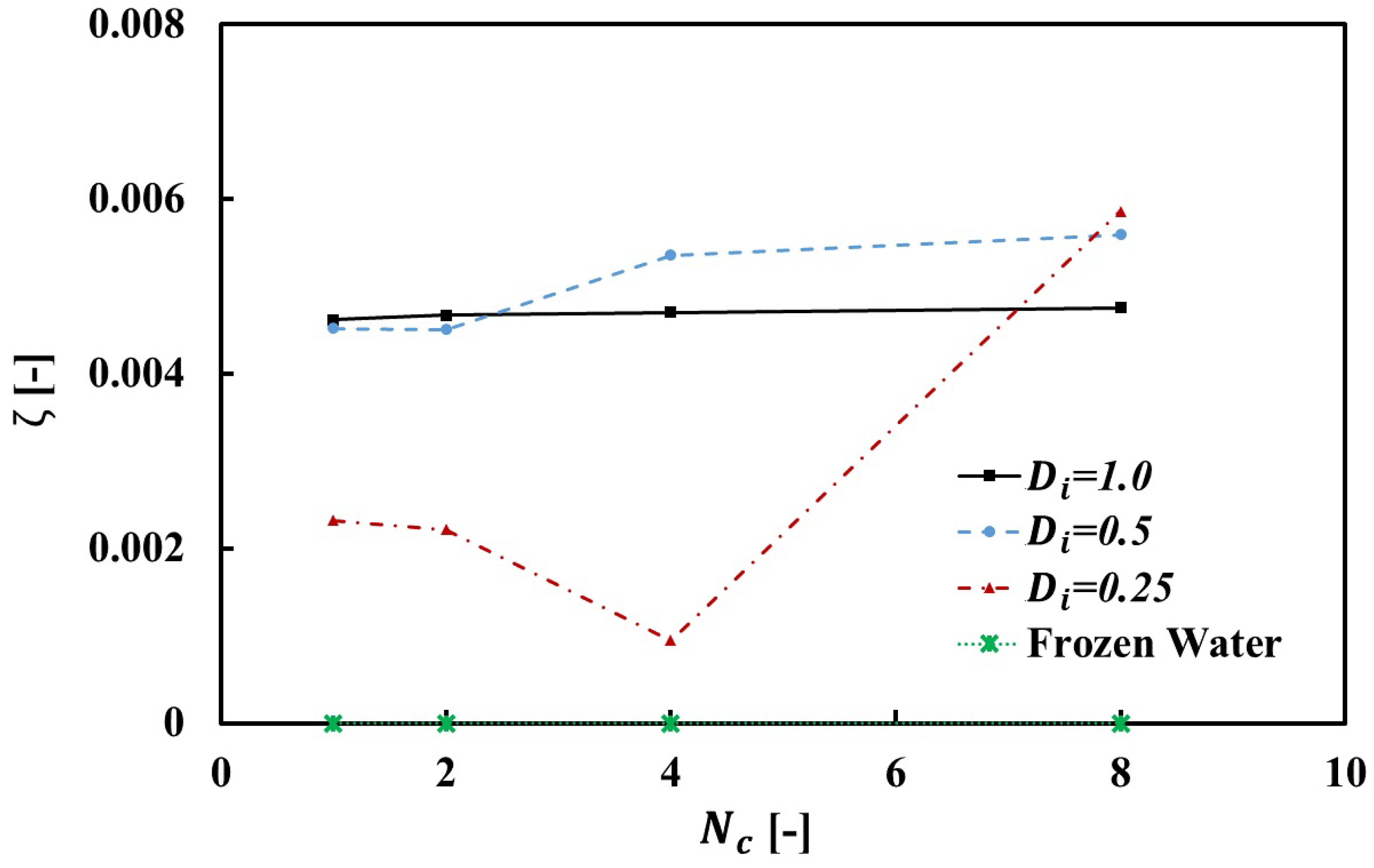
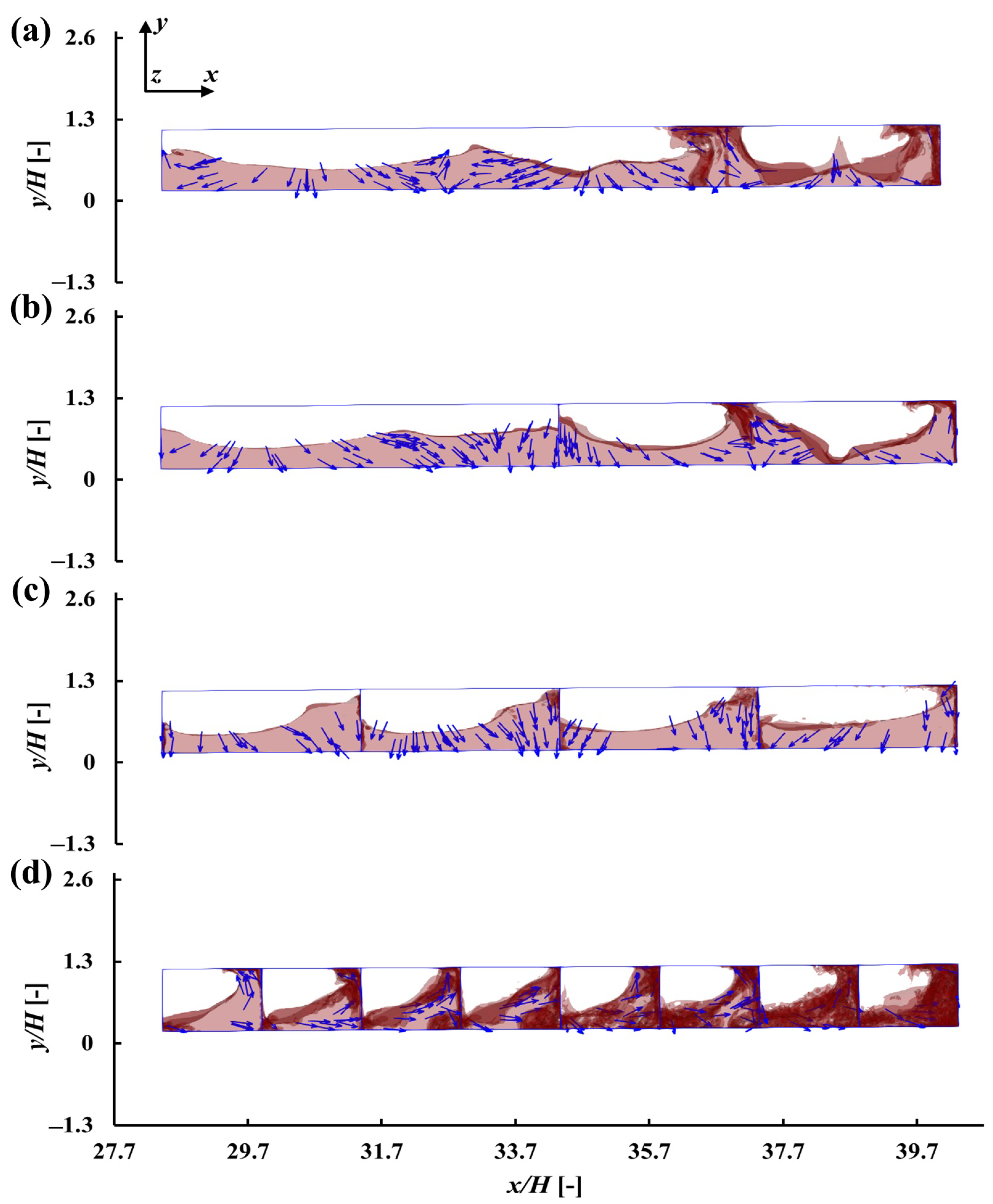
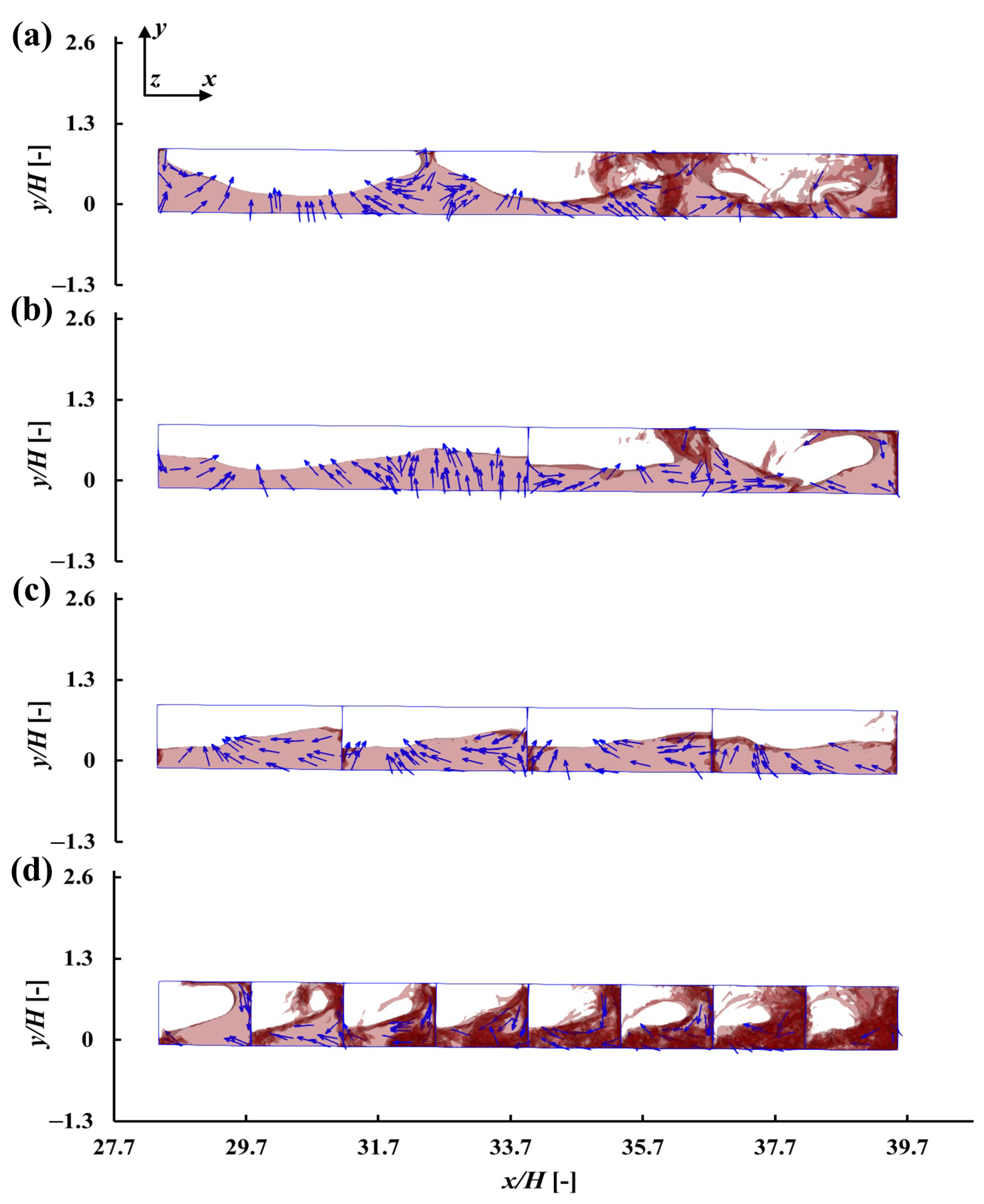
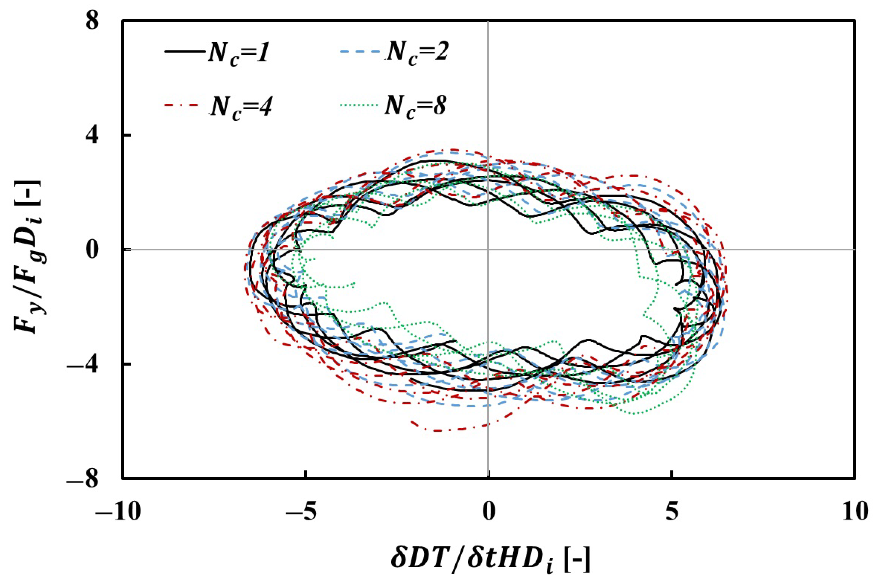
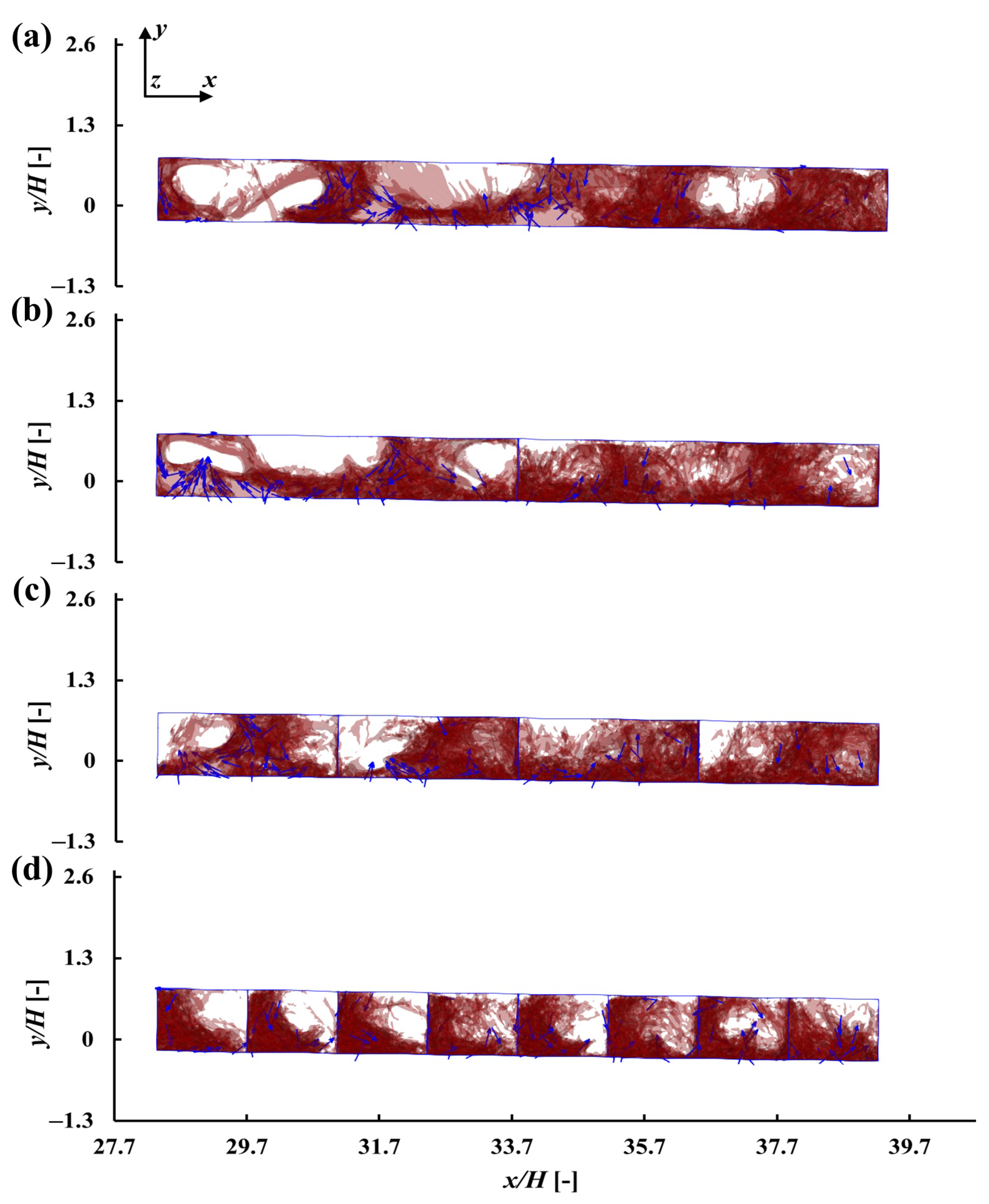
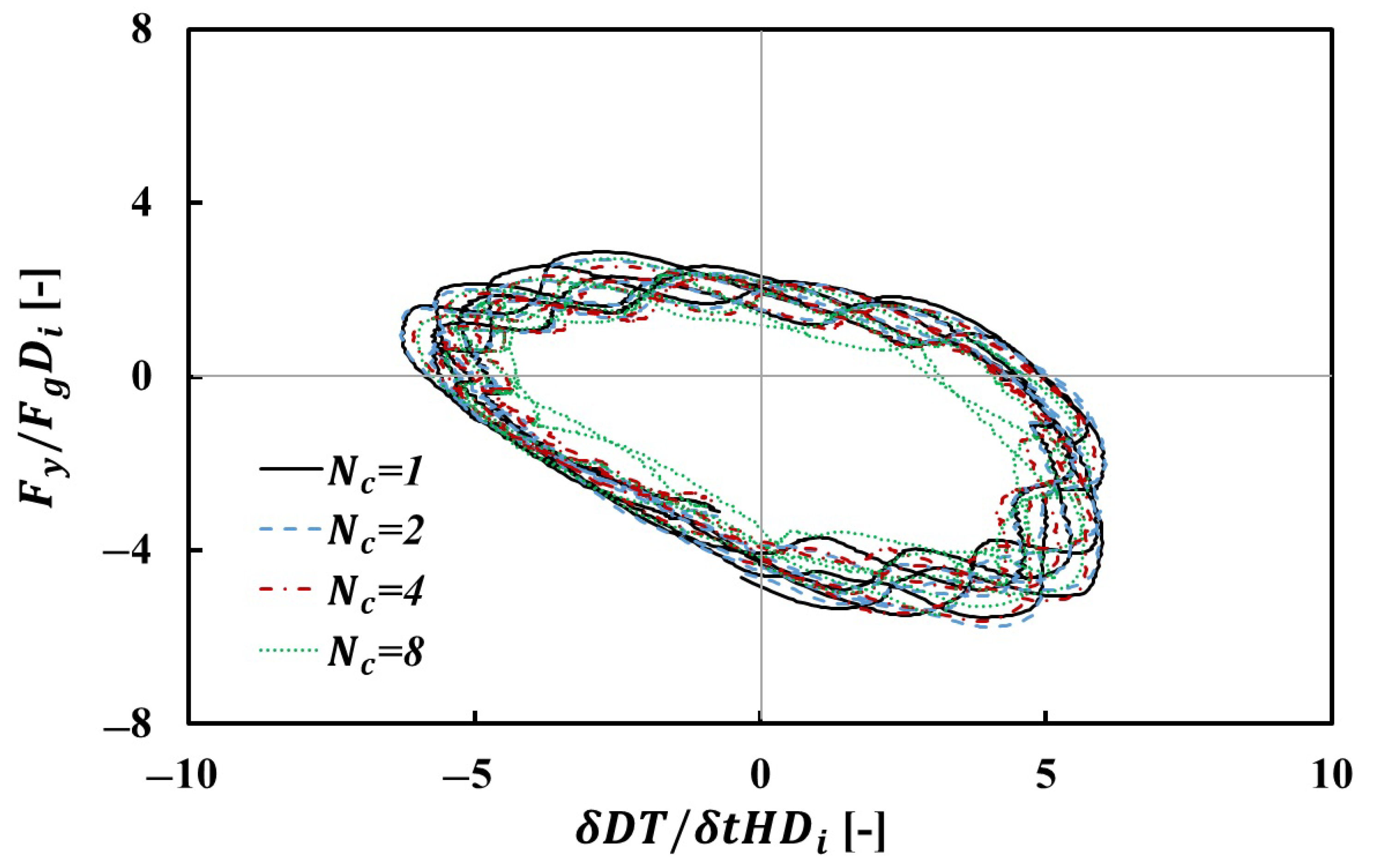
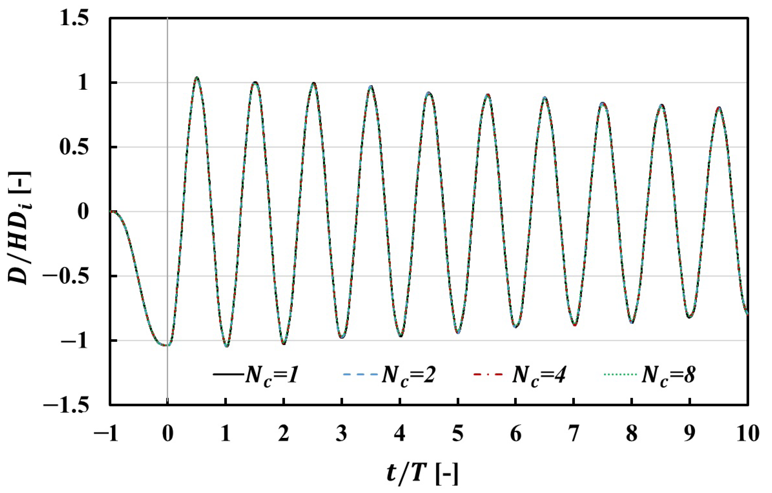
4.3. Impact of Compartment Numbers

The impact of compartment numbers on the slosh-induced damping ratio with three initial excitation displacements was also investigated. The instantaneous non-dimensional tip vertical displacement of the system over ten oscillation cycles for $D_i=0.25$ is shown in Figure 13. From the fifth cycle onwards, there is significant decay in the tip displacement with $N_c=8$, compared with other compartment numbers. In contrast, the tip displacement with $N_c=4$ decays less than other compartment numbers from the sixth cycle onwards.

Snapshots of the sloshing tank with $D_i=0.25$ with different compartment numbers during the sixth cycle (from $t/T=5.0$ to $t/T=6.0$) are shown in Figure 14, Figure 15 and Figure 16.

By placing a baffle in the middle of the tank (i.e., $N_c=2$), the formation of slosh wave is blocked. Due to the blockage of the mass and momentum exchange between the front and rear half of the tank, the amplitude of the wave crests with $N_c=2$ are smaller than that of the $N_c=1$. There is only one wave crest impact with the ceiling of the tank, but the impact is much more gentle than that of $N_c=1$ at $t/T=5.0$. A similar shape of sloshing waveform occurs for $N_c=2$ at $t/T=5.5$ and $t/T=6.0$ compared with that of $N_c=1$, but the waves formed in the rear half of the tank do not have contact with the tank ceiling at $t/T=6.0$.

By placing three baffles (i.e., $N_c=4$) in the water tank for $D_i=0.25$, the impact between the sloshing wave and the tank wall has been reduced. More specifically, at $t/T=5.0$, the tank of $D_i=0.25$ with $N_c=1$ and $N_c=2$ forms falling waves, but for the tank with $N_c=4$, as can be seen from Figure 14c, water has, and will, continue to fall to the front of its respective compartment along the slope. At $t/T=5.5$, falling waves are seen in all compartments with $N_c=4$, with gentle impact between the sloshing wave and the front top corner of each compartment for the front three. At $t/T=6.0$, when the tank is back to its lowest position, the free surfaces in all four compartments are generally horizontal.

As the number of compartments is increased to eight, we observe one sloshing wave cycle repeated over two cycles, with water slamming to the front and rear baffles and impacting the ceiling of the tank.

Different sloshing behaviour to that that has been observed under different compartment numbers is almost certainly due to changes in the natural frequency of the sloshing waves created by the different tank structures. According to Housner [52], the first sloshing frequency with rectangular tanks can be estimated by empirical equation as:

$$f_{slosh}=\frac{1}{2\pi }\sqrt{\frac{3.16g tanh\left(3.16\frac{h}{L}\right)}{L}}.$$

(9)

where $f_{slosh}$ is the first frequency, g is the gravitational acceleration, h is the height of the water tank and L is the length of the rectangular tank along direction of excitation. In this study, the water inside the tank is excited along both the longitudinal and the transverse directions due to the free decay motion of the cantilever beam. An increase in the number of compartments reduces the length of each in the longitudinal direction, hence, this increases the sloshing frequency. The slosh phenomenon we observed at $N_c=8$ is due to the sloshing frequency being approximately half of the beam’s oscillation frequency. While the beam oscillation frequency is not a multiple of the sloshing frequency when $N_c=4$; thus, a reduced impact between the sloshing wave and the tank wall is observed. An in-depth analysis of this behaviour is expected in future work.

From the snapshots in Figure 14 and Figure 16, the sloshing behaviour with eight compartments shows strong impacts with the ceiling and floor of the tank for all compartments in every oscillation cycle. This is reflected in Figure 17, which shows the normalised force-velocity diagram for the last five cycles with $D_i=0.25$. It can be seen that the vertical fluid force for $N_c=8$ is smaller than that with smaller compartment numbers in the third quadrant, likely due to the strong impact to the ceiling of the tank by the sloshing waves during the second half of the down stroke. A larger overall vertical fluid force in the fourth quadrant is also observed in the tank with $N_c=8$ compared with others, which is due to the interaction between the splash water and the floor of the tank during the first half of the upstroke.

It is also observed that the water tank with $N_c=4$ has larger vertical fluid force in the first and third quadrant compared with other cases. As discussed, this larger vertical fluid force is due to the lack of interaction between sloshing waves and the top/bottom walls of the tank of the misaligned sloshing frequencies and the oscillation frequency. A larger vertical fluid force in the first and third quadrant will bring less damping to the system. Less impact between the sloshing wave and the ceiling also makes the sloshing tank with $N_c=2$ have larger fluid force in both the first and third quadrant compared with that of $N_c=1$ and provide less damping to the system.

Figure 18 shows the instantaneous non-dimensional tip vertical displacement of the system over ten oscillation cycles for $D_i=0.5$. From the fifth oscillation cycle onwards, a clear decay in the tip displacement can be observed with $N_c=8$ and $N_c=4$, compared with $N_c=1$ and $N_c=2$.

Figure 19 and Figure 20 present snapshots of the sloshing tank with $D_i=0.5$ with different compartment numbers during the sixth cycle (from $t/T=5.0$ to $t/T=6.0$). Similar to findings in Figure 10 and Figure 11, the front half of the tank for $D_i=0.5$ and $N_c=1$ is dominated by the violent vertical motion. This agrees with observations from Figure 19a and Figure 20a at $t/T=5.0$ to $t/T=6.0$. By involving a baffle in the middle of the tank, as shown in Figure 19b and Figure 20b, the sloshing pattern is different from that with $N_c=1$, but the front half of the tank is also characterised by the turbulent vertical impacting motion, while in the rear half appears some waveform. By increasing the compartment number to four, although still highly turbulent, the water starts to display directional flow in all the compartments, instead of violent disordered turbulent behaviour. This is especially true for the front compartment.

If we take $t/T=5.5$ as an example (Figure 21c), the direction of motion for the water is to move to the rear of the compartment and then rush along the rear baffle to impact the ceiling of the tank. It should be noted that these directional flows for the sloshing tank with $N_c=4$ do not happen at every time instant. For example, at $t/T=5.0$, disordered turbulent motions are observed in the very front compartment, as shown in Figure 19c. For the sloshing tank with $N_c=8$ and $D_i=0.5$, a clear sloshing pattern, which is similar to that of $N_c=8$ and $D_i=0.25$, can be observed in Figure 19d and Figure 20d.

Figure 22 shows the normalised force–velocity diagram of the tank for the last five cycles with $D_i=0.5$ and four different compartment numbers. Similar to that of $D_i=0.25$, with the strong impact on the ceiling of the tank by the sloshing waves during the second half of the down stroke and the interaction between the splashing water and the floor of the tank during the second half of the upstroke, the fluid force for $N_c=8$ and $D_i=0.5$ is smaller with other cases in the third and first quadrants. This brings more damping to the system. For $N_c=4$, it can be observed that the vertical fluid force is marginally smaller than that of the $N_c=1$ in the second and third quadrant, with the existence of the directional flow as shown in Figure 21c and Figure 20c.

We further plotted the instantaneous non-dimensional tip vertical displacement of the system over ten cycles for $D_i=1.0$ in Figure 23. There is no significant difference that can be observed in the decay process of the beam–tank system for different compartment numbers.

As observed in Figure 8 and Figure 11, the sloshing pattern at $D_i=1.0$ and $N_c=1$ are dominated by the violent vertical motion from the third cycle onwards. As shown in Figure 24a–d, by placing baffles inside the water tank, the sloshing motion is also dominated by the violent vertical motion.

Figure 25 shows the normalised force–velocity diagram of the tank for the last five oscillation cycles with $D_i=1.0$ and four different compartment numbers. The force–velocity loops for different compartment numbers are very close to each other, with no significant difference that can be observed at $D_i=1.0$ compared with that at $D_i=0.5$ and $D_i=0.25$, which indicates that the damping provided by these sloshing tanks are similar. This is consistent with the results shown in Figure 4.

5. Conclusions

A preliminary investigation of the slosh-induced damping of an aircraft-wing-like structure was performed using a newly developed and open-source fluid–structure interaction framework. The first ten free-decay oscillation cycles were considered. We studied the impact of different excitation amplitudes and different numbers of compartments of the tank to slosh-induced damping. An idealised undamped cantilevered beam was employed to represent the aircraft-wing-like structure in order to make it possible to directly measure the slosh-induced damping from the time history of the tip displacement of the beam–tank system.

Three initial excitation amplitudes and four compartment numbers were studied. When the compartment number of the sloshing tank equals one, we observed a difference of less than 2% for slosh-induced damping according to the non-dimensional initial excitation amplitude, $D_i=1.0$ and $D_i=0.5$. This is more than two times larger than that of $D_i=0.25$. This is due to the strong impact on the ceiling and floor of the tank by the sloshing water during the free decay motion. The interaction between the sloshing wave crest and the tank wall is gentler under $D_i=0.25$, leading to small slosh-induced damping. By increasing the number of compartments within the tank, the slosh-induced damping of the system with $D_i=0.25$ reduced by 59% when using four tank compartments. This is due to a smaller impact between the tank ceiling and the wave crests due to the change in the sloshing wave frequency under this condition. When the compartment number of the beam–tank system with $D_i=0.25$ is increased to eight, the slosh-induced damping of the system increased by 153% due to the generation of large periodic sloshing waves with water slamming to the front and rear baffled regions and also due to impact with the ceiling of the tank.

For the beam–tank system with $D_i=0.5$, increasing the compartment number from one to eight also increases the slosh-induced damping due to a significant change in the sloshing pattern. For the beam–tank system with $D_i=1.0$, changing the number of compartments within the tank did not change the slosh-induced damping significantly within this study.

The present study focuses on the behaviour and slosh damping profile over the first ten cycles of the free decay oscillation; future work will look to understand this over longer oscillatory periods. The simplified structural model in the present beam–tank system will also be replaced by a more complex representation during the next phase of the study. In-depth analysis on sloshing frequencies with different compartments will be carried out, with the goal to obtain and analyse the forces in each individual compartment in order to allow for optimal design decisions in future wing design.

References

1. Ibrahim, R.A. Liquid Sloshing Dynamics: Theory and Applications; Cambridge University Press: Cambridge, UK, 2005. [Google Scholar]
2. Zheng, X.; You, Y.; Ma, Q.; Khayyer, A.; Shao, S. A comparative study on violent sloshing with complex baffles using the ISPH method. Appl. Sci. 2018, 8, 904. [Google Scholar] [CrossRef]
3. Jin, Q.; Xin, J.; Shi, F.; Shi, F. Parametric studies on sloshing in a three-dimensional prismatic tank with different water depths, excitation frequencies, and baffle heights by a Cartesian grid method. Int. J. Nav. Archit. Ocean. Eng. 2021, 13, 691–706. [Google Scholar] [CrossRef]
4. Cavalagli, N.; Biscarini, C.; Facci, A.L.; Ubertini, F.; Ubertini, S. Experimental and numerical analysis of energy dissipation in a sloshing absorber. J. Fluids Struct. 2017, 68, 466–481. [Google Scholar] [CrossRef]
5. Constantin, L.; De Courcy, J.; Titurus, B.; Rendall, T.C.; Cooper, J.E. Analysis of damping from vertical sloshing in a SDOF system. Mech. Syst. Signal Process. 2021, 152, 107452. [Google Scholar] [CrossRef]
6. Keulegan, G.H. Energy dissipation in standing waves in rectangular basins. J. Fluid Mech. 1959, 6, 33–50. [Google Scholar] [CrossRef]
7. Jiang, L.; Ting, C.L.; Perlin, M.; Schultz, W.W. Moderate and steep Faraday waves: Instabilities, modulation and temporal asymmetries. J. Fluid Mech. 1996, 329, 275–307. [Google Scholar] [CrossRef]
8. Jiang, L.; Perlin, M.; Schultz, W.W. Period tripling and energy dissipation of breaking standing waves. J. Fluid Mech. 1998, 369, 273–299. [Google Scholar] [CrossRef]
9. Tamura, Y.; Fujii, K.; Ohtsuki, T.; Wakahara, T.; Kohsaka, R. Effectiveness of tuned liquid dampers under wind excitation. Eng. Struct. 1995, 17, 609–621. [Google Scholar] [CrossRef]
10. Ikeda, T.; Nakagawa, N. Non-linear vibrations of a structure caused by water sloshing in a rectangular tank. J. Sound Vib. 1997, 201, 23–41. [Google Scholar] [CrossRef]
11. Bouscasse, B.; Colagrossi, A.; Souto-Iglesias, A.; Cercos-Pita, J. Mechanical energy dissipation induced by sloshing and wave breaking in a fully coupled angular motion system. I. Theoretical formulation and numerical investigation. Phys. Fluids 2014, 26, 033103. [Google Scholar] [CrossRef] [Green Version]
12. Bouscasse, B.; Colagrossi, A.; Souto-Iglesias, A.; Cercos-Pita, J. Mechanical energy dissipation induced by sloshing and wave breaking in a fully coupled angular motion system. II. Experimental investigation. Phys. Fluids 2014, 26, 033104. [Google Scholar] [CrossRef]
13. Merten, K.F.; Stephenson, B.H. Some Dynamic Effects of Fuel Motion in Simplified Model Tip Tanks on Suddenly Excited Bending Oscillations; Technical Report; 1952; Available online: https://digital.library.unt.edu/ark:/67531/metadc56319 (accessed on 3 June 2022).
14. Reese, J.R. Some Effects of Fluid in Pylon-Mounted Tanks on Flutter; Technical Report; 1955; Available online: https://digital.library.unt.edu/ark:/67531/metadc61466 (accessed on 3 June 2022).
15. Sewall, J.L. An Experimental and Theoretical Study of the Effect of Fuel on Pitching-Translation Flutter; Technical Report; 1957. Available online: https://ntrs.nasa.gov/citations/19930085017 (accessed on 3 June 2022).
16. Gambioli, F.; Chamos, A.; Jones, S.; Guthrie, P.; Webb, J.; Levenhagen, J.; Behruzi, P.; Mastroddi, F.; Malan, A.; Longshaw, S.; et al. Sloshing wing dynamics–project overview. In Proceedings of the 8th Transport Research Arena TRA 2020, Helsinki, Finland, 27–30 April 2020. [Google Scholar]
17. Gambioli, F.; Chamos, A.; Levenhagen, J.; Behruzi, P.; Mastroddi, F.; Malan, A.; Longshaw, S.; Skillen, A.; Cooper, J.E.; Gonzalez, L.; et al. Sloshing Wing Dynamics-2nd Year Project Overview. In Proceedings of the AIAA SCITECH 2022 Forum, San Diego, CA, USA, 3–7 January 2022; p. 1341. [Google Scholar]
18. Titurus, B.; Cooper, J.E.; Saltari, F.; Mastroddi, F.; Gambioli, F. Analysis of a sloshing beam experiment. In Proceedings of the International Forum on Aeroelasticity and Structural Dynamics, Savannah, GA, USA, 10–13 June 2019; Volume139. [Google Scholar]
19. Gambioli, F.; Usach, R.A.; Kirby, J.; Wilson, T.; Behruzi, P. Experimental evaluation of fuel sloshing effects on wing dynamics. In Proceedings of the 18th International Forum on Aeroelasticity and Structural Dynamics, Savannah, GA, USA, 10–13 June 2019. [Google Scholar]
20. Martinez-Carrascal, J.; González-Gutiérrez, L. Experimental study of the liquid damping effects on a SDOF vertical sloshing tank. J. Fluids Struct. 2021, 100, 103172. [Google Scholar] [CrossRef]
21. Constantin, L.; De Courcy, J.; Titurus, B.; Rendall, T.C.; Cooper, J.E. Sloshing induced damping across Froude numbers in a harmonically vertically excited system. J. Sound Vib. 2021, 510, 116302. [Google Scholar] [CrossRef]
22. Ilangakoon, N.A.; Malan, A.G.; Jones, B.W. A higher-order accurate surface tension modelling volume-of-fluid scheme for 2D curvilinear meshes. J. Comput. Phys. 2020, 420, 109717. [Google Scholar] [CrossRef]
23. Oomar, M.Y.; Malan, A.G.; Horwitz, R.A.; Jones, B.W.; Langdon, G.S. An all-Mach number HLLC-based scheme for multi-phase flow with surface tension. Appl. Sci. 2021, 11, 3413. [Google Scholar] [CrossRef]
24. Wright, M.D.; Gambioli, F.; Malan, A.G. CFD based non-dimensional characterization of energy dissipation due to verticle slosh. Appl. Sci. 2021, 11, 10401. [Google Scholar] [CrossRef]
25. Malan, A.G.; Jones, B.W.; Malan, L.C.; Wright, M. Accurate prediction of violent slosh loads via a weakly compressible vof formulation. In Proceedings of the 31st International Ocean and Polar Engineering Conference, Rhodes, Greece, 20–25 June 2021; OnePetro: Richardson, TX, USA, 2021. [Google Scholar]
26. Jones, B.W.A.; Wright, M.D.; Malan, A.G.; Farao, J.; Gambioli, F.; Lonshaw, S. A High Fidelity Fluid-Structure-Interaction Model of the Airbus Protospace Slosh Damping Experiment. In Proceedings of the International Forum on Aeroelasticity and Structural Dynamics, online, 13–17 June 2022. [Google Scholar]
27. Calderon-Sanchez, J.; Martinez-Carrascal, J.; Gonzalez-Gutierrez, L.; Colagrossi, A. A global analysis of a coupled violent vertical sloshing problem using an SPH methodology. Eng. Appl. Comput. Fluid Mech. 2021, 15, 865–888. [Google Scholar] [CrossRef]
28. De Courcy, J.J.; Constantin, L.; Titurus, B.; Rendall, T.; Cooper, J.E. Gust Loads Alleviation Using Sloshing Fuel. In Proceedings of the AIAA Scitech 2021 Forum, Online, 11–15, 19–21 January 2021; p. 1152. [Google Scholar]
29. Pizzoli, M.; Saltari, F.; Mastroddi, F.; Martinez-Carrascal, J.; González-Gutiérrez, L.M. Nonlinear reduced-order model for vertical sloshing by employing neural networks. Nonlinear Dyn. 2022, 107, 1469–1478. [Google Scholar] [CrossRef]
30. Mastroddi, F.; Saltari, F.; Traini, A.; Barile, A.; Gambioli, F. Sloshing ROMs for Fluid-Structure Interactions in Aerospace Applications. In Proceedings of the AIAA Scitech 2020 Forum, Orlando, FL, USA, 6–10 January 2020; p. 1451. [Google Scholar]
31. Liu, W.; Longshaw, S.M.; Skillen, A.; Emerson, D.R.; Valente, C.; Gambioli, F. A High-Performance Open-Source Solution for Multiphase Fluid-Structure Interaction. Int. J. Offshore Polar Eng. 2022, 32, 24–30. [Google Scholar] [CrossRef]
32. Liu, W. ParaSiF—Parallel Partitioned Multi-physics Simulation Framework. Available online: https://github.com/ParaSiF/ParaSiF (accessed on 3 June 2022).
33. Liu, W.; Longshaw, S.M.; Skillen, A.; Emerson, D.R.; Valente, C.; Gambioli, F. A High-Performance Open-Source Solution for Multiphase Fluid-Structure Interaction. In Proceedings of the The Thirty-first International Ocean and Polar Engineering Conference (ISOPE-2021), Rhodes, Greece, 20–25 June 2021; OnePetro: Richardson, TX, USA, 2021. [Google Scholar]
34. Weller, H.G.; Tabor, G.; Jasak, H.; Fureby, C. A tensorial approach to computational continuum mechanics using object-oriented techniques. Comput. Phys. 1998, 12, 620–631. [Google Scholar] [CrossRef]
35. Alnæs, M.; Blechta, J.; Hake, J.; Johansson, A.; Kehlet, B.; Logg, A.; Richardson, C.; Ring, J.; Rognes, M.E.; Wells, G.N. The FEniCS project version 1.5. Arch. Numer. Softw. 2015. [Google Scholar] [CrossRef]
36. Tang, Y.; Kudo, S.; Bian, X.; Li, Z.; Karniadakis, G. Multiscale Universal Interface: A Concurrent Framework for Coupling Heterogeneous Solvers. J. Comput. Phys. 2015, 297, 13–31. [Google Scholar] [CrossRef]
37. Tuković, Ž.; Karač, A.; Cardiff, P.; Jasak, H.; Ivanković, A. OpenFOAM finite volume solver for fluid-solid interaction. Trans. FAMENA 2018, 42, 1–31. [Google Scholar] [CrossRef]
38. Jasak, H. Dynamic mesh handling in OpenFOAM. In Proceedings of the 47th AIAA Aerospace Sciences Meeting Including the New Horizons Forum and Aerospace Exposition, Orlando, FL, USA, 5–8 January 2009; p. 341. [Google Scholar]
39. Hirt, C.W.; Nichols, B.D. Volume of fluid (VOF) method for the dynamics of free boundaries. J. Comput. Phys. 1981, 39, 201–225. [Google Scholar] [CrossRef]
40. Rusche, H. Computational Fluid Dynamics of Dispersed Two-Phase Flows at High Phase Fractions. Ph.D. Thesis, Imperial College London (University of London), London, UK, 2003. [Google Scholar]
41. Erlicher, S.; Bonaventura, L.; Bursi, O.S. The analysis of the generalized-α method for non-linear dynamic problems. Comput. Mech. 2002, 28, 83–104. [Google Scholar] [CrossRef]
42. Bleyer, J. Numerical Tours of Computational Mechanics with Fenics. Zenodo 2018. Available online: http://comet-fenics.readthedocs.io/en/latest/intro.html (accessed on 20 October 2021).
43. Newmark, N.M. A method of computation for structural dynamics. J. Eng. Mech. Div. 1959, 85, 67–94. [Google Scholar] [CrossRef]
44. Slyngstad, A.S. Verification and Validation of a Monolithic Fluid-Structure Interaction Solver in FEniCS. A Comparison of Mesh Lifting Operators. Master’s Thesis, University of Oslo, Oslo, Norway, 2017. [Google Scholar]
45. Rendall, T.C.; Allen, C.B. Unified fluid–structure interpolation and mesh motion using radial basis functions. Int. J. Numer. Methods Eng. 2008, 74, 1519–1559. [Google Scholar] [CrossRef]
46. Bungartz, H.J.; Lindner, F.; Gatzhammer, B.; Mehl, M.; Scheufele, K.; Shukaev, A.; Uekermann, B. preCICE—A fully parallel library for multi-physics surface coupling. Comput. Fluids 2016, 141, 250–258. [Google Scholar] [CrossRef]
47. Liu, W.; Wang, W.; Skillen, A.; Longshaw, S.; Moulinec, C.; Emerson, D. A parallel partitioned approach on fluid-structure interaction simulation using the multiscale universal interface coupling library. In Proceedings of the 14th WCCMECCOMAS Congress, Virtual Congress, 11–15 January 2021; Volume 1400. [Google Scholar]
48. Liu, W.; Wang, W.; Skillen, A.; Fernandez, E.R.; Longshaw, S.; Sawko, R. Code Development on Parallel Partitioned Fluid-Structure Interaction Simulations. 2020. Available online: https://epubs.stfc.ac.uk/work/46400815 (accessed on 3 June 2022).
49. Schneider, T.; Hu, Y.; Gao, X.; Dumas, J.; Zorin, D.; Panozzo, D. A large scale comparison of tetrahedral and hexahedral elements for finite element analysis. arXiv 2019, arXiv:1903.09332. [Google Scholar]
50. Tahmasebi, M.K.; Shamsoddini, R.; Abolpour, B. Performances of different turbulence models for simulating shallow water sloshing in rectangular tank. J. Mar. Sci. Appl. 2020, 19, 381–387. [Google Scholar] [CrossRef]
51. Huang, W.; He, T.; Yu, J.; Wang, Q.; Wang, X. Direct CFD Simulation and Experimental Study on Coupled Motion Characteristics of Ship and Tank Sloshing in Waves. In Proceedings of the International Conference on Offshore Mechanics and Arctic Engineering, Hamburg, Germany, 5–10 June 2022; Volume 85185, p. V008T08A035. [Google Scholar]
52. Housner, G.W. Dynamic Analysis of Fluids in Containers Subjected to Acceleration. In Nuclear Reactors and Earthquakes; Report No. TID; 1963; Volume 7024, Available online: https://digital.library.unt.edu/ark:/67531/metadc1030393/m2/1/high_res_d/4620608.pdf (accessed on 3 June 2022).
Figure 1. Schematic of the simplified elastic aircraft-wing-like structure consisting of a hollow cantilevered steel beam with a sloshing water tank.
Applsci 12 08481 g001
Figure 2. Schematic of the open-source framework, ParaSiF, with the two-way implicit FSI coupling scheme.
Applsci 12 08481 g002
Figure 3. Meshes used for the simulation of the free decay of an oscillating aircraft-wing-like structure with a sloshing tank with (a) fluid mesh and (b) structure mesh.
Applsci 12 08481 g003
Figure 4. Damping ratio of the free decay beam–tank system with both sloshing water and frozen water as a function of the number of compartments.
Applsci 12 08481 g004
Figure 5. Time history of non-dimensional (a,c) tip vertical displacement and (b,d) vertical fluid force of the system over ten oscillation cycles with one compartment, in which (c,d) are normalised by the initial excitation amplitude.
Applsci 12 08481 g005
Figure 6. Snapshots for the sloshing tank with D i = 1.0 and N c = 1 at (a) t / T = 0.0 and (b) t / T = 0.5 . Water phase is shown as transparent red with dark red representing the free surface. Blue arrows show the general direction of motion of the sloshing water.
Applsci 12 08481 g006
Figure 7. Snapshots for the sloshing tank with N c = 1 at t / T = 2.0 for (a) D i = 0.25 , (b) D i = 0.5 and (c) D i = 1.0 . Water phase is shown as transparent red with dark red representing the free surface. Blue arrows show the general direction of motion of the sloshing water. The three subplots are points A 0.25 , A 0.5 and A 1.0 , respectively, which are presented in Figure 9.
Applsci 12 08481 g007
Figure 8. Snapshots for the sloshing tank with N c = 1 at t / T = 2.5 for (a) D i = 0.25 , (b) D i = 0.5 and (c) D i = 1.0 . Water phase is shown as transparent red with dark red representing the free surface. Blue arrows show the general direction of motion of the sloshing water. The three subplots are points B 0.25 , B 0.5 and B 1.0 , respectively, that presented in Figure 9.
Applsci 12 08481 g008
Figure 9. Normalised force-velocity diagram for the third oscillation cycle with N c = 1 .
Applsci 12 08481 g009
Figure 10. Snapshots for the sloshing tank with N c = 1 at t / T = 7.0 for (a) D i = 0.25 , (b) D i = 0.5 and (c) D i = 1.0 . Water phase is shown as transparent red with dark red representing the free surface. Blue arrows show the general direction of motion of the sloshing water.
Applsci 12 08481 g010
Figure 11. Snapshots for the sloshing tank with N c = 1 at t / T = 8.0 for (a) D i = 0.25 , (b) D i = 0.5 and (c) D i = 1.0 . Water phase is shown as transparent red with dark red representing the free surface. Blue arrows show the general direction of motion of the sloshing water.
Applsci 12 08481 g011
Figure 12. Normalised force–velocity diagram for the eighth and ninth oscillation cycles with N c = 1 .
Applsci 12 08481 g012
Figure 13. Time history of non-dimensional tip vertical displacement of the system normalised by the initial excitation amplitude over ten cycles for D i = 0.25 .
Applsci 12 08481 g013
Figure 14. Snapshots for the sloshing tank with D i = 0.25 at t / T = 5.0 for (a) N c = 1 , (b) N c = 2 , (c) N c = 4 and (d) N c = 8 . Water phase is shown as transparent red with dark red representing the free surface. Blue arrows show the general direction of motion of the sloshing water.
Applsci 12 08481 g014
Figure 15. Snapshots for the sloshing tank with D i = 0.25 at t / T = 5.5 for (a) N c = 1 , (b) N c = 2 , (c) N c = 4 and (d) N c = 8 . Water phase is shown as transparent red with dark red representing the free surface. Blue arrows show the general direction of motion of the sloshing water.
Applsci 12 08481 g015
Figure 16. Snapshots for the sloshing tank with D i = 0.25 at t / T = 6.0 for (a) N c = 1 , (b) N c = 2 , (c) N c = 4 and (d) N c = 8 . Water phase is shown as transparent red with dark red representing the free surface. Blue arrows show the general direction of motion of the sloshing water.
Applsci 12 08481 g016
Figure 17. Normalised force–velocity diagram for the last five oscillation cycles with D i = 0.25 .
Applsci 12 08481 g017
Figure 18. Time history of non-dimensional tip vertical displacement of the system normalised by the initial excitation amplitude over ten cycles for D i = 0.5 .
Applsci 12 08481 g018
Figure 19. Snapshots for the sloshing tank with D i = 0.5 at t / T = 5.0 for (a) N c = 1 , (b) N c = 2 , (c) N c = 4 and (d) N c = 8 . Water phase is shown as transparent red with dark red representing the free surface. Blue arrows show the general direction of motion of the sloshing water.
Applsci 12 08481 g019
Figure 20. Snapshots for the sloshing tank with D i = 0.5 at t / T = 6.0 for (a) N c = 1 , (b) N c = 2 , (c) N c = 4 and (d) N c = 8 . Water phase is shown as transparent red with dark red representing the free surface. Blue arrows show the general direction of motion of the sloshing water.
Applsci 12 08481 g020
Figure 21. Snapshots for the sloshing tank with D i = 0.5 at t / T = 5.5 for (a) N c = 1 , (b) N c = 2 , (c) N c = 4 and (d) N c = 8 . Water phase is shown as transparent red with dark red representing the free surface. Blue arrows show the general direction of motion of the sloshing water.
Applsci 12 08481 g021
Figure 22. Normalised force–velocity diagram for the last five oscillation cycles with D i = 0.5 .
Applsci 12 08481 g022
Figure 23. Time history of non-dimensional tip vertical displacement of the system normalised by the initial excitation amplitude over ten cycles for D i = 1.0 .
Applsci 12 08481 g023
Figure 24. Snapshots for the sloshing tank with D i = 1.0 at t / T = 5.5 for (a) N c = 1 , (b) N c = 2 , (c) N c = 4 and (d) N c = 8 . Water phase is shown as transparent red with dark red representing the free surface. Blue arrows show the general direction of motion of the sloshing water.
Applsci 12 08481 g024
Figure 25. Normalised force–velocity diagram for the last five oscillation cycles with D i = 1.0 .
Applsci 12 08481 g025
Publisher’s Note: MDPI stays neutral with regard to jurisdictional claims in published maps and institutional affiliations.