Effect of Fuel Sloshing on the Damping of a Scaled Wing Model—Experimental Testing and Numerical Simulations

Abstract

Vertical sloshing of liquid-filled tanks has been shown to induce substantial dissipative effects. Building upon these previous results obtained on simpler sloshing systems, a scaled wing prototype is presented here, equipped with a fuel tank that allows the observation of liquid sloshing and quantification of induced dynamic effects. Based on experiments conducted at a 50% filling level for a baffled wing fuel tank model, substantial additional damping effects were demonstrated with liquid inside the tank regardless of the vertical acceleration amplitude. A numerical model based on a finite element wing structural model and a surrogate 1DOF fluid model was explored, with numerical simulations showing good agreement compared to experiments throughout the decaying motion of the system.

1. Introduction

Aircraft designed and developed in the European zone must comply with the certification specifications of the European Aviation Safety Agency (EASA). According to the Certification Specifications for Large Aeroplanes (CS-25) Acceptable Means of Compliance (AMC), the structural dynamic model of the aircraft may include damping information: “In the absence of better information it will normally be acceptable to assume 0.03 (i.e., 1.5% equivalent critical viscous damping) for all flexible modes. Structural damping may be increased over the 0.03 value to be consistent with the high structural response levels caused by extreme gust intensity, provided justification is given.” [1]. The value of the structural damping may be increased if justified, and a larger value of structural damping may lead to a less conservative structural design through reduction in the peak loads and/or improving the fatigue life of certain components. These improvements, in turn, lead to a more efficient use of materials, reduced weight and improved fuel burn, in line with the current trends toward a reduction in the environmental impact of aviation (e.g., the ATAG net-zero carbon goal by 2050 (https://www.atag.org/component/news/?view=pressrelease&id=125, accessed on 12 July 2022)).

A conventional approach for aircraft load alleviation uses control surfaces (often spoilers or ailerons), actuated using an active control law to reduce the dynamic response of the aircraft to gusts and manoeuvres. More recently, there have been proposals for passive load alleviation using tow-steered composites [2] or folding wing-tips [3]. Another possible candidate for reductions in dynamic aircraft loads is fuel sloshing inside wings, taking into account and exploiting the movement of the fuel inside large aircraft wings. A net increase in damping may be achieved due to the dynamic interaction between the moving fuel and the wing structure. This work is part of Sloshing Wing Dynamics (SLOWD), an EU-funded project (https://slowd-project.eu/project/project_overview, accessed on 12 July 2022) aiming to investigate and exploit fuel sloshing in order to increase the effective damping in aircraft structures.

The experimental work presented here is based on extensive previous investigations into systems of reduced complexity, and part of it was also previously presented in [4]. A transient single degree of freedom analysis was conducted in [5], where an experimental analysis supported by two numerical models of varying fidelity showed that (1) vertical sloshing induces substantial damping effects that depend on the tank filling level and amplitude of excitation, and (2) qualitatively and quantitatively, different sloshing dissipation mechanisms are present at large and small amplitudes of excitation. Similar findings were reported in [6]. An in-depth experimental and numerical analysis based on single-frequency harmonic excitation [7,8] then revealed how the liquid movements relative to the tank affect the observed induced effects.

High fidelity numerical models are considered in the SLOWD project, based on Smoothed Particle Hydrodynamics (SPH) and Volume of Fluid (VoF) CFD that have proven their modelling capability on 1DOF vibrating systems [5,9] and on beam systems [10]. Multiple reduced-order numerical models for sloshing were considered as well. Vertical sloshing action was modelled using bouncing balls [5], ballistic-harmonic kinematics-based models [7] and bouncing ball models trained on experimental data using neural networks [11]. The numerical approach taken in this work is based on extensive experimental characterisation of vertical damping at large amplitudes over multiple frequencies, based on which a surrogate model is interpolated.

Using the insights and analysis developed in the previous studies, this work represents a step up in the analysis complexity considering the liquid sloshing-induced effects in a scaled research wing prototype. While previous studies have considered single degree of freedom systems, liquid sloshing inside aircraft wings involves spanwise acceleration gradients, more complex tank geometries and a multi-modal response. Here, step release tests on a sloshing wing model are presented with a 50% filling level and equivalent frozen mass conditions. A numerical model based on sloshing response surfaces from 1DOF experiments is introduced, emphasising induced damping similarities across geometric scales.

This paper is organised as follows: the research methodology is presented in Section 2, and the experimental and numerical results concerning the dry and wet structure are presented and discussed in Section 3 and Section 4. Conclusions and future directions of work are presented in Section 5.

2. Methodology

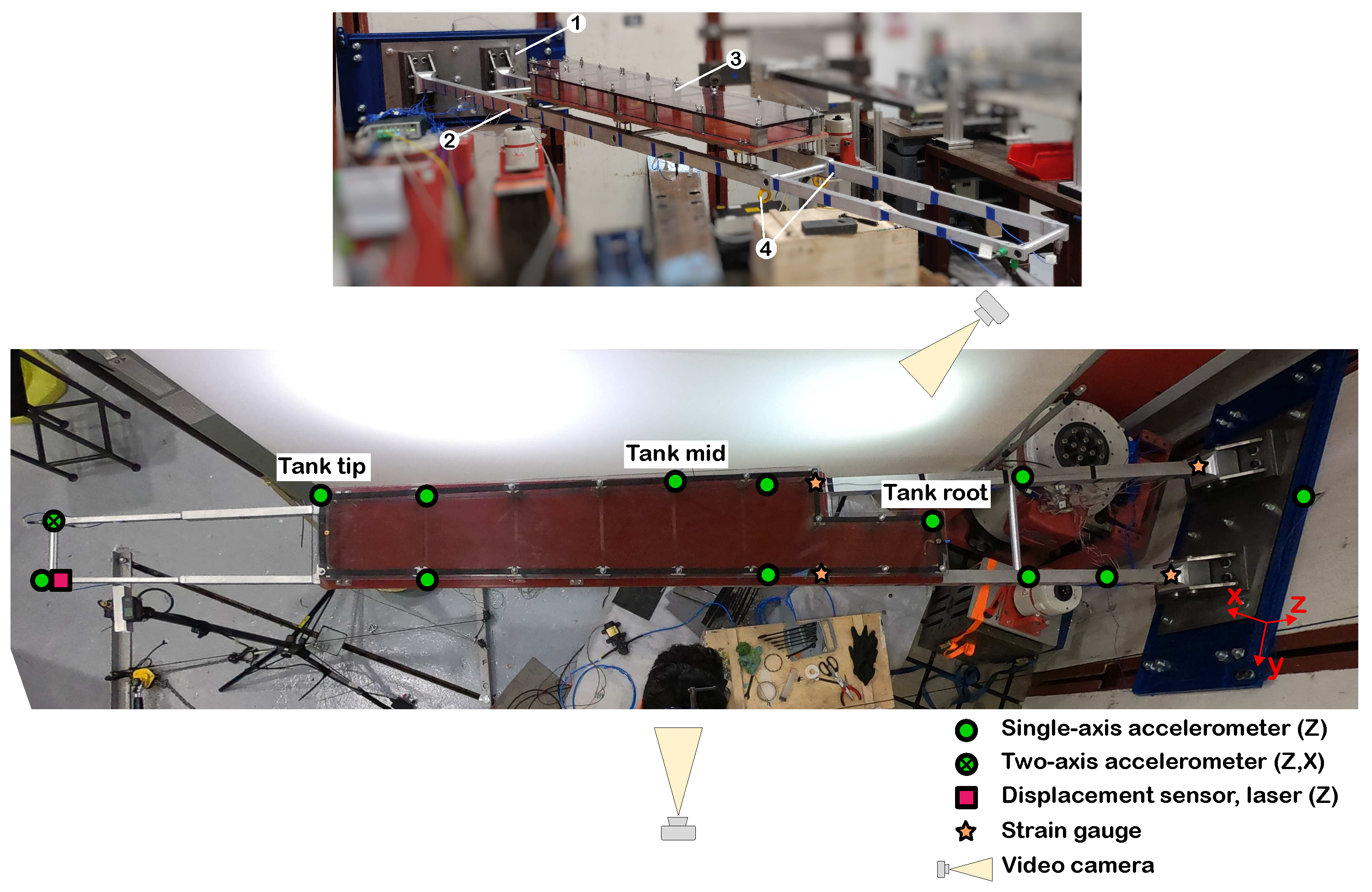
2.1. Experimental Methodology

The experimental work in the SLOWD project followed an incremental development in experimental complexity and cost: single degree of freedom sloshing tests [5], sloshing beam tests [12], scaled wing model and planned full-scale wing sloshing tests. The current experimental campaign is concerned with the experimental demonstrator called “MiniWoT” (miniature wing of tomorrow), shown in Figure 1. The model is a 1:5 geometric scale wing structure with some particular features that allow for fuel sloshing investigations. The main structural part is composed of two spars and five torque tubes with spanwise varying cross-sectional properties to match the static and dynamic response of a full-scale research prototype wing specimen, as described in [13]. The structure is approximately 3 m long and is cantilevered at the root to a strong wall using a wedge-bracket configuration that enables the modification of the specimen dihedral angle (shown here in $0^{\circ }$ dihedral configuration). On top of the main structural part, there is a transparent fuel tank with scaled geometry. The tank bears only part of the loads, and it is partially decoupled from the main structural part using two rigid connection points and five flexure-type connections that allow for limited spanwise relative motion between the tank and the underlying structure. This configuration was chosen with multiple aims in mind, among the most important: (1) achieve set natural frequencies and mode shapes, (2) allow for the liquid flow observation inside the tank from the lateral and top directions and (3) the tank should have set scaled dimensions and spanwise position, representative of the full-scale specimen. It can easily be seen how such requirements impose certain design constraints that move the fuel tank vertically up from its natural position inside the wing as well as raise considerable challenges concerning the connection points between the tank and the underlying structure.

The fuel tank has a geometry representative of the full-scale prototype with 8 interior cells (numbered in this work from 1 to 8 starting from the inboard position) separated by the baffles. The seven baffles are removable, and multiple baffle geometries can be studied. The individual cells can also be sealed using the solid-section baffles without perforations—this case is considered in this work.

The structure is instrumented using 14 accelerometers, one vertical displacement measurement at the tip trailing edge, strain gauges at the root and two high frame rate video cameras for the observation of the sloshing liquid from the side and top of the tank. Three of the accelerometers were placed on the tank in three different spanwise positions, as shown in Figure 1 and labelled “tank tip”, “mid” and “root”. Two removable eye bolts (labelled as (4) in Figure 1) and a pulley–chain hoist mechanism were used for loading the structure vertically downward, after which it was released into free decaying motion using a pin-release mechanism.

The experimental test plan included but was not limited to the following:

• Ground vibration tests with and without tank attached, part of which was presented in [13],
• Step release tests without liquid (dry tests), with and without additional mass to account for the “frozen” liquid,
• Step release tests with tap water as the working liquid, with and without added dye
• Studies with and without the baffles, with the baffles of different solidity ratios,
• Studies with varying filling levels.

This work presents an initial assessment and interpretation of the experimental results concerning step release tests at a $0^{\circ }$ dihedral angle, with $50\%$ water filling level in each individual sealed cell using solid-section baffles, and the equivalent dry case with added mass to account for the liquid. The choice for the treatment of the 50% filling level case is based on previous experimental and numerical studies, which have shown [5] that sloshing-induced damping is maximised at 50% fill in vertically vibrating transient systems, when only the vertical component of motion is isolated. Water was used as the working liquid since previous studies have shown that the liquid viscosity has little influence on the sloshing-induced damping effects [9]. Each test was conducted at least three times to assess its repeatability.

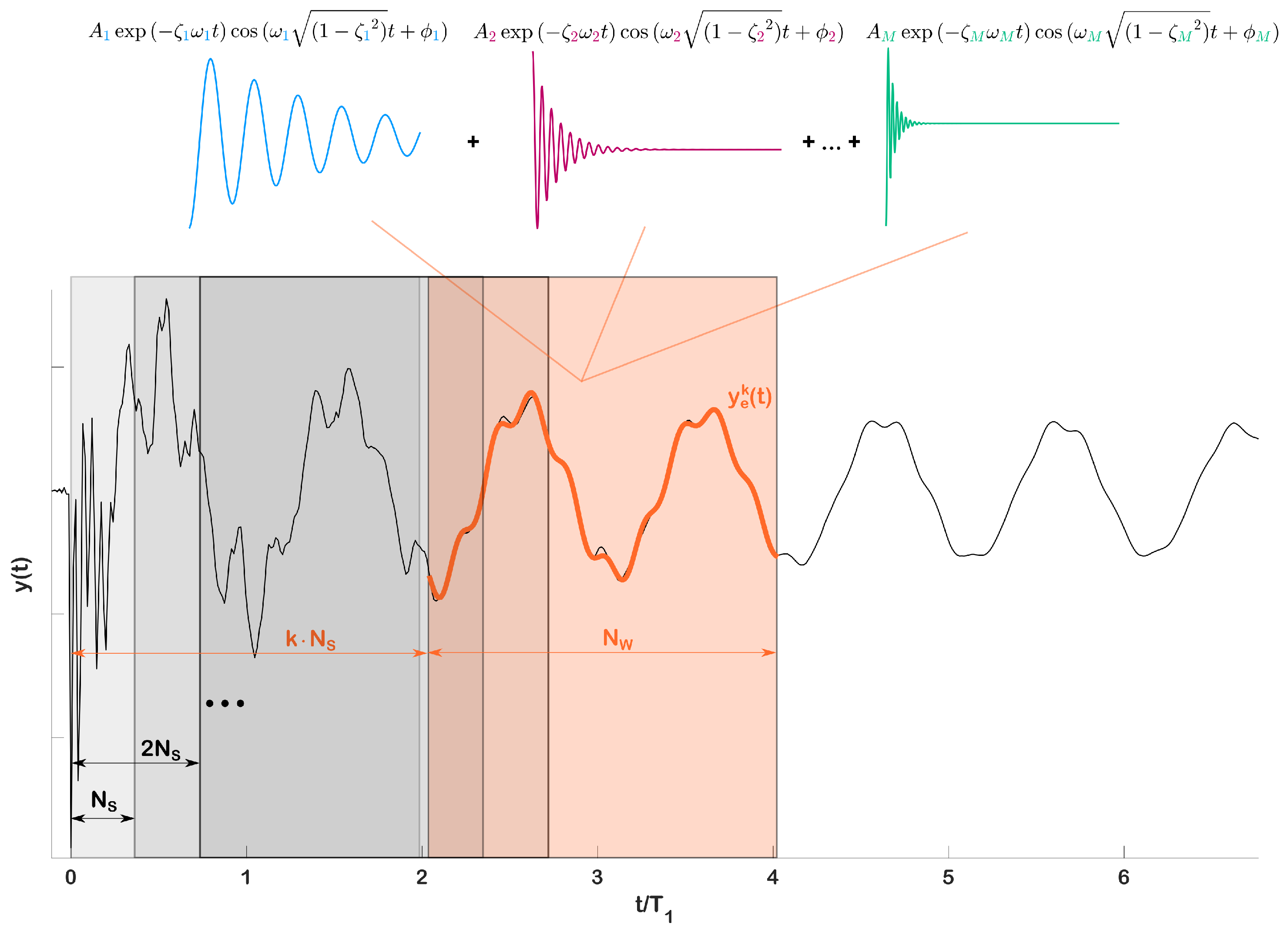
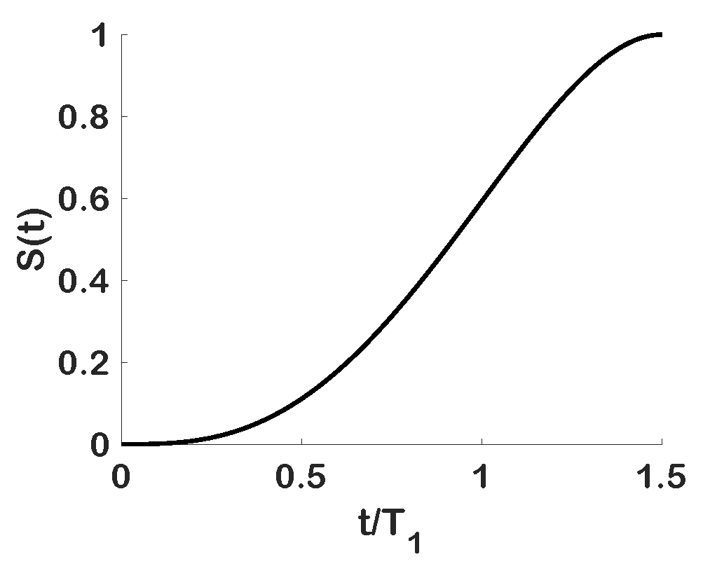
2.1.1. Nonlinear System Identification

The transient MiniWoT experimental responses considered in this work exhibit moderately nonlinear stiffness effects and highly nonlinear induced damping; due to these characteristics, the system identification problem is not trivial. Many nonlinear system identification techniques have classically been proposed and used, e.g., based on the Volterra series or block-structured nonlinear models consisting of interconnected linear and nonlinear subsystems [14]. Due to the nature of the problem at hand, piecewise linear modelling is adopted here. Such approaches assume time-localised linear behaviour, allowing the application of well-known linear techniques to the short sections of the time-domain response of the studied nonlinear system. The piecewise linear system can be found using the fitting techniques, which minimize the distance between the signal and chosen fitting functions in a least squares sense. Such methods belong to a class of Nonlinear Least Squares (NLS) fitting techniques and have been successfully used in the past for the analysis of one dominant frequency component in beam sloshing experiments [12]. We extend the NLS analysis here to cover all major frequency components of the transient signals, and a description of the method as applied in this work follows.

Let $F1$ be the natural frequency of vibration of the first bending mode of the MiniWoT structure, as identified by studying the small amplitude vibrations of the structure. The time-dependent acceleration data $y\left(t\right)$ contains approximately 75 samples of data per one period of motion $T1=1/F1$. The size of the data bin is chosen to be $N_W\approx 150$ samples, corresponding to 2 periods of motion of the first vibration mode of the structure. A classical damped multi-harmonic motion representation

$$y_e=\sum _{j=1}^M\left[A_{j}exp(-{\zeta }_j{\omega }_{j}t)cos({\omega }_j\sqrt{1-{{\zeta }_j}^2}t+{\varphi }_j)\right]$$

(1)

is fitted to the signal inside each data bin in a least squares sense, where M is the number of frequency components considered to be dominant in the step release response. Each signal component j is characterised by its amplitude $A_j$, damping ratio ${\zeta }_j$, frequency ${\omega }_j$ and phase ${\varphi }_j$. Figure 2 exemplifies this methodology, showing the signal binning and decomposition. The black curve represents the original signal $y\left(t\right)$. Starting from $t=0$, a bin of length $N_W$ is selected, an estimate $y_e\left(t_1\right)$ is obtained for bin number 1 using M signal components and then the bin slides by $N_S$ samples, after which the procedure is repeated. The signal at time $t_k$ will thus be described by the function $y_e^k\left(t\right)$. The length of the sliding distance $N_S$ establishes the time resolution of the analysis and is chosen such that each frequency component of interest can be studied at a sufficient level of detail while also keeping the computation relatively inexpensive. The value of $N_S$ is exaggerated in Figure 2 for clarity; for the results presented in this work, $N_S=4$ is used. The result of this analysis will identify the nonlinear system using the vectors $A_j$, ${\zeta }_j$, ${\omega }_j$ and ${\varphi }_j$ of size N, where N is the number of fitted functions $y_e$ over all time bins.

Since this nonlinear identification procedure is developed for transient signals, different signal components j will be attenuated at different rates characterised by ${\zeta }_j$. The main challenge of this type of analysis is to ensure its robustness while multiple frequency components gradually disappear from the signal $y\left(t\right)$. The problem that arises is that the basic form of the curve fitting algorithm will try to fit all frequency components at all times, even though the respective components may not be meaningfully present in the signal anymore due to their drop below the noise floor. This leads to instabilities in the fitting algorithm, which in turn causes spurious oscillations in the terms $A_j$, ${\zeta }_j$, ${\omega }_j$ and ${\varphi }_j$, leading to an ambiguous identification of the system parameters. This problem is solved by adding a series of ad hoc constraints imposed on the parameter search space, specifically:

• The amplitude of each component is limited at $2y\left(0\right)$.
• The frequency of each component is limited in the interval $(1\pm x)·{\omega }_j\left(0\right)$, where ${\omega }_j\left(0\right)$ is the linear estimate of the frequency component and x is the frequency deviation allowed for.
• If the damping ratio of one component ${\zeta }_j$ exceeds a threshold value (set here at 0.9, or $90\%$ of critical damping), the respective component is eliminated from the signal estimate $y_e$ for all subsequent bins.

These constraints do not limit the parameter search space excessively and effectively regularise the search procedure when operating on the noisy data. Constraint #1 ensures that no amplitude exceeds two times the initial acceleration at the step release point; note that the likelihood of any component reaching such values under free vibrations is low. Constraint #2 ensures that the identified frequency component will be found only in the relative vicinity ($\pm 10\%$ was used here) of the linear estimate, while still allowing for significant nonlinear effects to be manifested by the frequency shifts. Further, note that for the well-separated frequency components, this constraint can be relaxed or eliminated completely. Finally, constraint #3 is instrumental in ensuring the robustness and stability of the algorithm. Previously, it was observed that when the component j has a negligibly small presence in the signal in the bin number k, the returned values for both $A_j\left(k\right)$ and ${\zeta }_j\left(k\right)$ increased steeply. Of course, this local increase did not affect the other components since the j-th amplitude was very low at this point. However, if left unchecked, this behaviour led to ever-increasing parameter values and oscillatory solutions, which ultimately affected the overall stability of the analysis. The threshold value $\zeta =0.9$ is well above the expected damping ratios for any frequency component and, as such, it does not overconstrain the analysis.

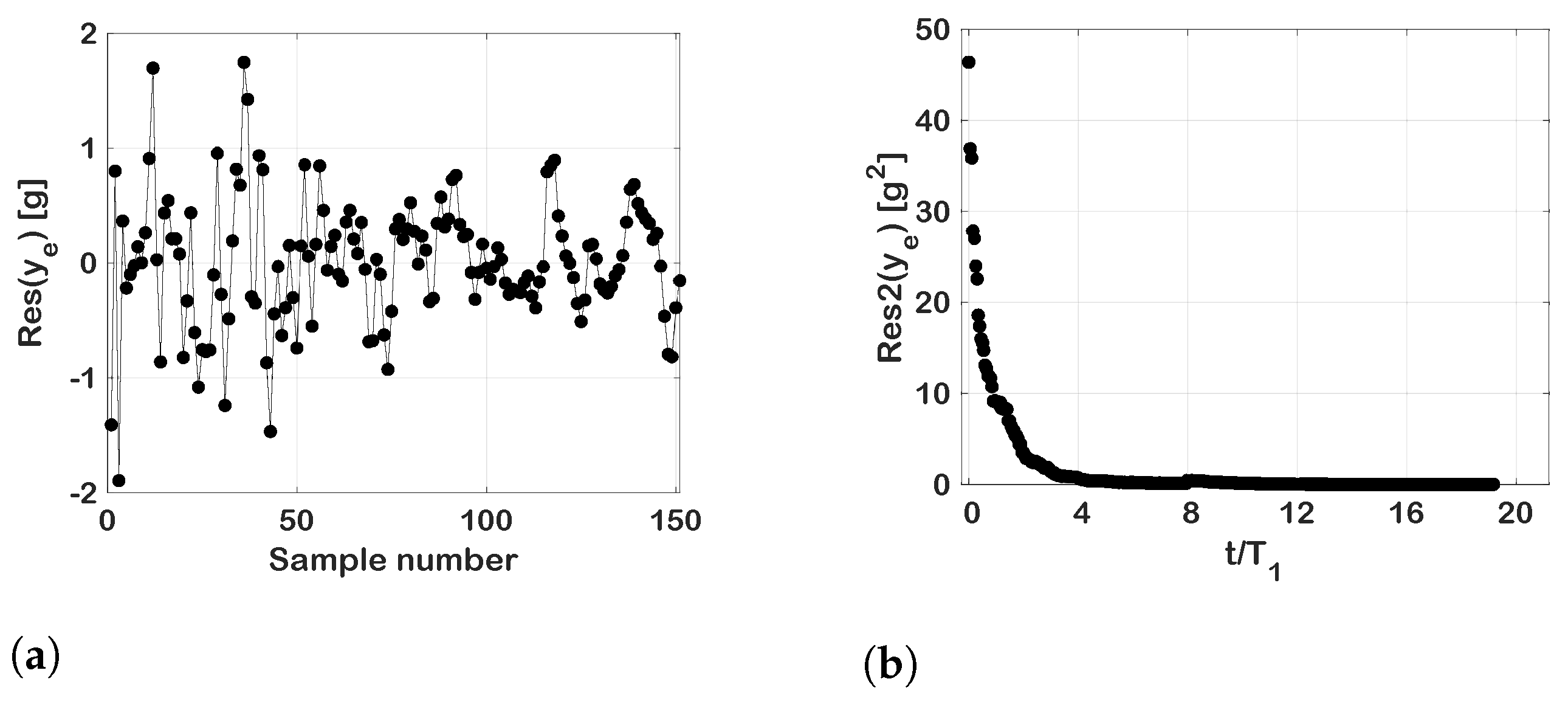
2.1.2. Example of Miniwot Data Curve Fitting

Before proceeding further, consider an example system identification result for one of the experimental cases studied in this work, showing the quality of the fitted results. Figure 3 shows an example of the acceleration signal at the tip of the fuel tank for a representative dry MiniWoT test. The original experimental data are shown in black; the reconstructed signal is shown in green, obtained by piecing together all of the $y_e^k\left(t\right)$ signals in each time bin, as exemplified in Figure 2. A very good match is seen by the overlap of the two curves at all times. The insets also show details of the signal trace in time, indicating the damping of the higher frequency components at different rates until only the first bending mode is dominant.

The suitability of the identification technique can also be quantified using the residuals. The residuals for each fitted function are computed as

$$Res\left(y_e\right)=y\left(t\right)-y_e\left(t\right)$$

(2)

and the sum of squares of the residuals (SSR) in a bin is

$$Res2\left(y_e\right)=\sum _{i=1}^{N_W}{\left(y\left(t\right)-y_e\left(t\right)\right)}^2$$

(3)

with the units of acceleration squared.

An example of residuals for this analysis is shown in Figure 4 for the fitting case shown in Figure 3. Figure 4a shows the residuals for the first fitted function immediately after t = 0 for each sample inside the bin of length $N_W$, while Figure 4b shows the SSR (summed squared residuals) values for all data bins, e.g., the first point represents the SSR for the bin shown in Figure 4a. Residuals of approximately 10% of the maximum acceleration value can be seen in the first fitted bin, and the squared residuals are dropping together with the amplitude of the signal, as expected. The fitting error is largest in the first cycle of motion due to the very rich frequency content following immediately after the step release event. Such values for the residuals are common for this type of piecewise linear analysis [15]. Correlating these results with the qualitative view in Figure 3, we conclude that this method is able to parameterise the damped transient responses accurately. Its utility for interpreting the studied processes will be illustrated in the following sections.

Before moving forward, it is important to discuss one possible limitation of the damping ratio identification specifically relevant in extremely nonlinear circumstances. The damping ratio of a particular physical system may exhibit amplitude-dependent nonlinearities such that the values ${\zeta }_j$ change substantially (nonlinearly) within the duration of a single data bin, i.e., one or two periods of motion in this case. Because of the linear response assumption within a single data bin (implying a constant ${\zeta }_j$), the choice of the bin size $N_W$ can lead to the smearing and averaging effect on the ${\zeta }_j$ values when traversing this region. Thus, the identified damping estimate may be weighted by the consecutive or neighbouring damping values in such highly nonlinear instances. Further, it was found that a data bin of the length less than the two periods of motion of the lowest frequency leads to substantial oscillations in the solution for the cases presented here. Consequently, we assume constant ${\zeta }_j$ values over the two fundamental periods of motion. Here, as well as in other instances of time-frequency analysis, there is a compromise to be made between the time resolution of the analysis and the robustness of the damping estimation.

2.2. Numerical Methodology

This section presents a numerical model of the overall coupled fluid-structure problem based on a combination of a MiniWoT finite element representation and a novel surrogate model of the vertical forces generated by the sloshing fluid.

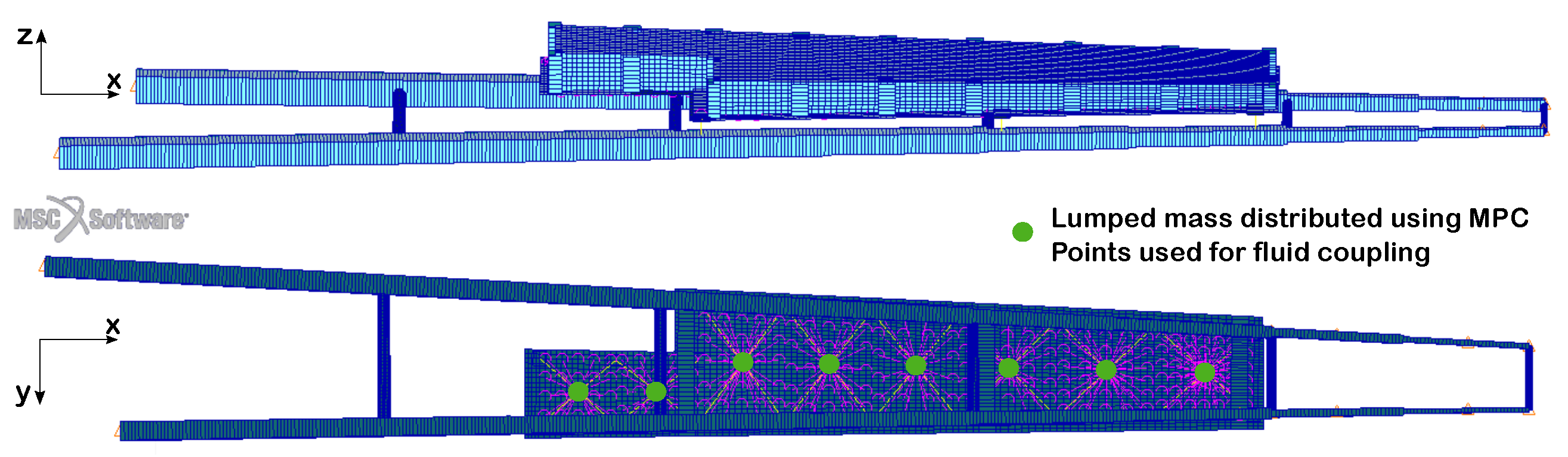
2.2.1. Structural Model

The structural model consists of a linear modal model that uses 12 normal modes obtained from a Nastran [16] finite element model (FEM). MSC Patran [17] was used for mesh generation and pre-processing of the FEM, and the model is shown in Figure 5, with the types and number of elements shown in

Table 1. FE model elements and nodes.

Element Type	Nastran Element	Number of Elements
Plate	CQUAD4	10,147
Beam	CBEAM	1200
Spring	CBUSH	17
Spring	CELAS1	6
Mass	CONM2	55
MPC	RBE3	22
Number of nodes	10,903

. The underlying structure was modelled using beam elements, the tank using shell elements and beams for the side pillars (also see Figure 1), and the spring elements were used to model the flexibility of the spar-torque tube, root and tank connections. Multi-point constraints (MPC) of type RBE3 were used to distribute the lumped dry mass on the bottom of the tank and also, later, to distribute the effect of the liquid force. The Nastran FEM was calibrated for the structure without the tank (see [13]) and partially calibrated for the structure with the tank to achieve a very good match in the first two out-plane bending modes. This is sufficient for the present analysis, where the fluid has the most significant influence on the out-of-plane dynamics. Here, we describe how the Nastran normal modes solution is extracted and used in a way that provides a simple generalised framework to perform various transient fluid-structure coupled simulations.

Modal analysis of the FE model computes a matrix of normal mode shapes $\mathbf{\psi }$ and vector of the relevant structural frequencies $\underline{\omega }$, which can be used to form the generalised mass and stiffness matrices. Assuming mass normalised mode shapes, the structural equations of motion take the form

$$\mathit{I}\underline{\ddot{q}}+\mathit{C}\underline{\dot{q}}+\mathit{K}\underline{q}={\underline{F}}_q,\mathit{K}=\mathrm{diag}\left({\underline{\omega }}^2\right),\mathit{C}=\mathrm{diag}\left(2\underline{\zeta }\underline{\omega }\right)$$

(4)

where $\underline{q}$ is the vector of modal displacements, $\mathit{I}$ the identity matrix, $\mathit{K}$ and $\mathit{C}$ the generalised stiffness and modal damping matrix, respectively and ${\underline{F}}_q$ the vector of applied forcing in the modal space. The damping ratios of individual modes of vibration are identified from ground vibration tests. Whilst this model is sufficient at capturing small magnitude vibrations (where the $\underline{\zeta }$ values are identified), it is insufficient at representing the large amplitude vibration damping where the structure displays significant nonlinear characteristics. It is not straightforward to decide what type of nonlinear terms to include in this case. In recent years, there has been substantial analytical work conducted on “generalised” oscillators with noninteger order stiffness and damping. For example, in [18], the single degree of freedom model with nonlinear damping and nonlinear elastic forces of any order (integer or noninteger) was studied and then extended to multiple degrees of freedom in [19]. Possible applications are envisaged in the correct modelling of micro-electromechanical systems dynamics. Here, we use a similar approach where we consider the damping powers as optimisation parameters allowed to be nonintegers. The numerical model can thus capture the nonlinear experimental dry damping without much concern about the physical meaning of each term, which is not of direct interest in this current work. Therefore, this modification leads to the final set of equations of motion used in this investigation

$$\mathit{I}\underline{\ddot{q}}+{\alpha }_1\mathit{C}\underline{\dot{q}}+\mathit{K}\underline{q}={\mathit{\psi }}^{\mathrm{T}}{\underline{F}}_{ext}+{\mathit{\psi }}^{\mathrm{T}}{\underline{F}}_s-{\alpha }_2\mathit{C}\mathrm{sign}\left(\underline{\dot{q}}\right)|\underline{\dot{q}}{|}^{{\beta }_2}-{\alpha }_3\mathit{C}\mathrm{sign}\left(\underline{\dot{q}}\right){\left|\underline{\dot{q}}\right|}^{{\beta }_3}$$

(5)

where ${\underline{F}}_{ext}$ and ${\underline{F}}_s$ are the global vectors of applied external and internal sloshing forces, respectively, defined in Cartesian coordinates at the FE nodes. Equation (5) is recast in state space such that time integration can be performed in Matlab using the Runge–Kutta 45 pair implemented within the ODE45 solver [20].

Parameters ${\alpha }_{1-3}$ and ${\beta }_{2-3}$ define the nonlinear damping response of the dry MiniWoT model. These parameters were determined by solving an optimisation problem that minimises the differences between the numerical and experimental damping ratios obtained from the response time series following the free-release conditions whilst only considering the out-of-plane dynamics. The resulting damping parameters can be found in

Table 2. Optimised damping parameters of the numerical model.

Parameter	${\mathit{\alpha }}_1$	${\mathit{\alpha }}_2$	${\mathit{\alpha }}_3$	${\mathit{\beta }}_2$	${\mathit{\beta }}_3$
Value	4.71	0.70	1.29	2.64	3.63

. This simplified equivalent nonlinear damping model is used to capture the global dissipative properties arising from significantly more complex nonlinear internal and external influences such as boundary conditions, joint interfaces and aerodynamics effects.

Figure 6 shows the comparison between the experimental data and the calibrated model for the frozen mass case. On the left-hand side, the tank tip acceleration versus time normalised by the first bending mode period is shown, and on the right hand side, the acceleration amplitude of the first bending component is shown on a semi-logarithmic scale. There is a very good match overall, indicative of the fact that the model frequencies and damping correspond well with the experimental measurement. The logarithm of the acceleration envelope shows damping trends in the first signal component (calibrated). For the viscous damping case, such a curve is a line on a semi-logarithmic plot; this is not the case here, indicative of dry damping nonlinearity that is correctly captured by the numerical model.

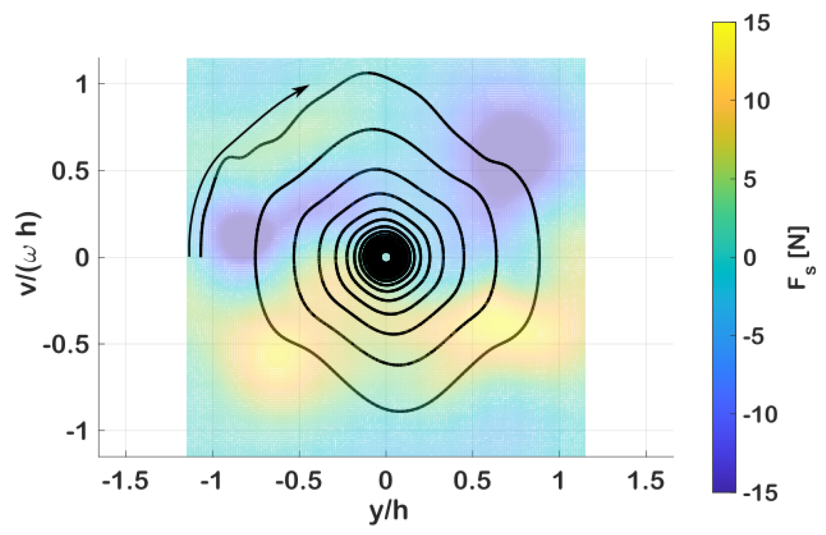
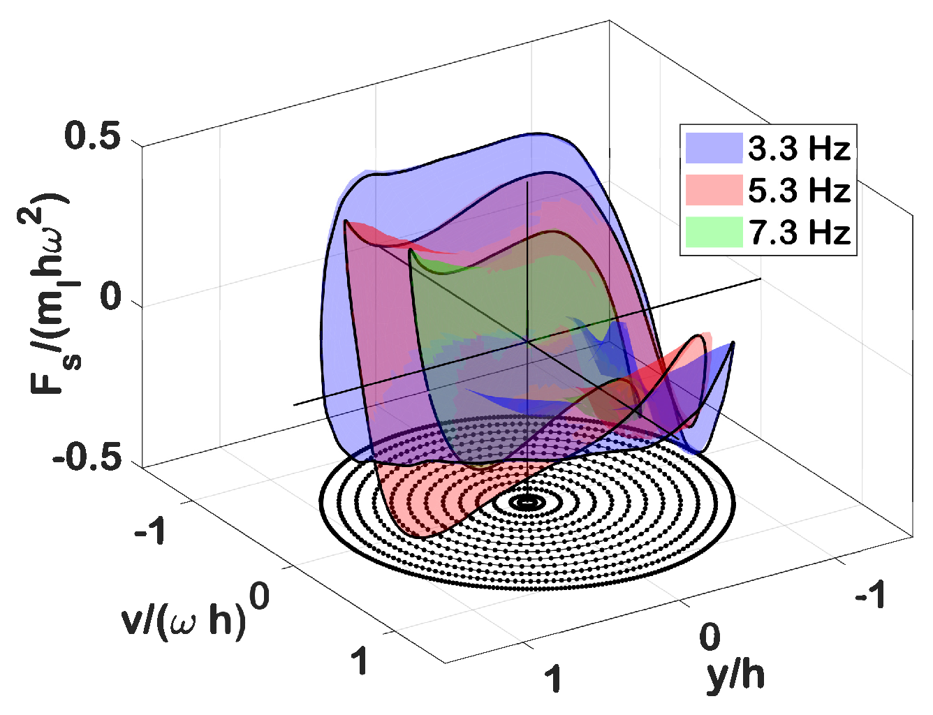
2.2.2. Quasi-Steady Model of the Transversal Sloshing Force

To capture dissipative effects arising from the fluid during interaction with the structure, a fluid model must be chosen that can apply representative forcing onto the structure based on the kinematic excitation within each tank cell. Classically, reduced-order models (ROM) of fluid behaviour are employed based on linearised fluid equations or equivalent mechanical models (EMM) such as swinging pendula or mass-spring-damper systems that represent free-surface displacement and fluid impacting [21,22]. However, these models are often limited to lateral fluid motion or linear and weakly-nonlinear free-surface motions. In response to this, EMMs have recently been developed to capture fluid response under large amplitude vertical excitation, such as the bouncing ball model [5,23] and ballistic-harmonic model [7]. These provide a good representation of dissipative and interactional behaviour of a fluid during the violent impacting regime but struggle to capture low-amplitude parametric sloshing. More recently, high-fidelity computational fluid dynamics approaches have been used, which are not limited by the magnitude of excitation nor tank geometry effects but, in turn, suffer from complex software coupling requirements and long execution times. Therefore, this section describes a recently developed vertical sloshing ROM, which can capture accurate hydrodynamic forces over a range of kinematic excitation magnitudes and sloshing response regimes with minimal computational overhead.

The reduced-order sloshing model subsequently discussed is based upon the direct application of experimentally identified sloshing forces in a manner comparable to surrogate modelling; therefore, it is prudent to introduce the experimental studies that are the basis of this model. Previous work has focused on identifying sloshing motions and damping characteristics from prescribed, vertical, harmonic excitation of a rectangular fluid-filled tank [7], where the vertical harmonic motion was chosen to replicate the out-of-plane bending dynamics that are typically seen in wing-like structures. In doing so, the total force acting on the fluid and tank structure was recorded to analyse the hysteretic force-displacement loops that define energy dissipation within the system. By removing the hydrostatic and inertial component from the total force, a resultant “sloshing” force remains due to the presence of a dynamic medium inside the tank. Specifically,

$$F_s=F_t-\ddot{y}(m_l+m_s)-g(m_l+m_s)$$

(6)

where $m_l$ and $m_s$ are the liquid and structural masses, respectively. For a fixed amplitude and frequency of excitation, this sloshing force was measured and averaged across multiple cycles (following the initial transient), resulting in the “quasi-steady” sloshing force, which acts at each kinematic condition within the prescribed cycle,

$$y=Asin\left(\omega t\right),v=A\omega cos\left(\omega t\right)\Rightarrow {\overline{F}}_s=g(y,v,A,\omega )sin\left(\omega t\right)$$

(7)

Each prescribed cycle can be visualised as a single circle in the x–y plane of Figure 7. When the experimental analysis is performed over multiple amplitudes, it forms a series of discrete circles, and therefore, a 3D landscape of the sloshing force. The applicability of this analysis for fluid-structure coupled simulation is immediately noticeable; as a structure undergoes transverse motion, the vertical kinematics of the tank can be tracked, and the relevant nonlinear sloshing force returned to the structure. Further, the range of amplitudes in the experimental data ensures multiple fluid regimes are included, from little free-surface motion (R3), low amplitude Faraday waves (R2) and violent fluid impacting (R1). However, a series of caveats to this particular method must be addressed, namely

• Scaling between the experimental and numerical (MiniWoT) tank dimensions.
• Producing a continuous and smooth sloshing force for numerical analysis, which can not be directly extracted from the experimental data. A result of the finite sampling frequency producing discrete data points in each cycle, plus discrete amplitudes and frequencies of the harmonic cycles considered.
• Identified forces assume the fluid has reached a quasi-steady state under the excitation and, therefore, can not account for sharp transients (i.e., free-release of the structure). A mechanism must be introduced to account for the initial energy input into the fluid to excite the identified motions within the data-set.

Here, scaling laws are based purely on non-dimensional kinematic and force terms, namely displacement $\widehat{y}=y/h$, velocity $\widehat{v}=\dot{y}/\left({\omega }_{c}h\right)$ and force ${\widehat{F}}_s=F_s/\left(m_{l}h{\omega }^2\right)$, where the characteristic length is tank height h, $m_l$ the liquid mass and $\omega$ the characteristic frequency of excitation for that specific excitation condition. Within the previous experimental work [7], normalisation of dissipated energy via $\widehat{E}=E/\left(m_l{\omega }^2{A}^2\right)$, where A is the amplitude of harmonic excitation, was shown to provide a consistent scaling across excitation conditions. However, generally in the transient setting, a characteristic amplitude is not known a priori; hence, the characteristic length of tank height is used. The significant assumption made is that the fluid forcing (and thus, resulting dissipation characteristics) scales with these non-dimensional terms. No scaling for the tank geometry (aside from height) is considered, which is generally less problematic for the violent impacting regime (R1) but becomes more important during the R2 regime, where the formation of standing waves is sensitive to the base geometry of the tank. This is further discussed later and has a direct influence on the chosen fluid parameters used within this particular analysis. Further, the dissipation resulting from the hydrodynamic response is likely to increase with tank scales (increasing $m_l$) due to increased free-surface fragmentation and volumetric dissipation forming from turbulent eddies in the liquid. Whilst not included here, a correctly introduced Froude scaling could approximate these effects [24].

Regarding the second point, the discrete experimental data must be applied to the numerical model in a continuous and smooth fashion to ensure successful time integration. Therefore, radial basis function interpolation is used, an established method for providing accurate and robust scattered-data interpolation of n-dimensional data [25]. Initially, consider the total experimental data set across multiple amplitudes and frequencies of excitation, the function mapping excitation kinematics to sloshing force can take the form ${\widehat{\underline{F}}}_s=\widehat{g}\left(\widehat{\mathit{x}}\right),\widehat{\mathit{x}}=\{\widehat{\underline{y}},\widehat{\underline{v}},\underline{\omega }\}$. The RBF interpolation, including a polynomial of any degree, provides the interpolated function values $\widehat{g}\left(\widehat{x}\right)$ at an evaluation point ${\widehat{x}}_E$,

$$\widehat{g}\left({\widehat{x}}_E\right)=\sum _{j=1}^N{\gamma }_i\varphi \left(\right|{\widehat{x}}_E-{\widehat{x}}_i|,r)+\sum _{k=1}^M{\lambda }_k{p}_k\left({\widehat{x}}_E\right)$$

(8)

where N is the number of experimental data points, p the M monomial coefficients based on the degree of the included polynomial and dimensionality of the data and $\varphi$ a compact basis function (a Wendland C4 is used) dependent on a spatial support length r. Following the standard RBF interpolation procedure [25], model coefficients $\gamma$ and $\lambda$ are found by requiring exact recovery of the experimental/sample points, requiring a solution to the linear system

$$\left(\begin{array}{cc}\mathit{\varphi }& \mathit{P}\\ {\mathit{P}}^{\mathrm{T}}& \mathbf{0}\end{array}\right)\left(\begin{array}{c}\underline{\gamma }\\ \underline{\lambda }\end{array}\right)=\left(\begin{array}{c}\underline{\widehat{g}}\hfill \\ \underline{0}\hfill \end{array}\right)$$

(9)

where $\mathit{\varphi }$ is an $N\times N$ matrix of basis function terms evaluated between each data point, $\mathit{P}$ an $M\times N$ matrix of the monomial terms, $\underline{\widehat{g}}$ a vector of the known non-dimensional sloshing forces. This interpolation ensures the experimental data points are exactly recovered and returns to a least-squares polynomial fit in the absence of RBF influence. However, in the current experimental data set, the polynomial term has little influence, and only a constant polynomial term is considered to avoid over-fitting and false extrapolation of the experimental data. Additionally, to improve matrix conditioning and simplify dependence on support radius r in N-dimensional space, the experimental domain ($\widehat{\mathit{x}}$) is scaled to the hypercube.

The solution to Equation (9) and subsequent application of Equation (8) to find the sloshing force at each tank can be used directly in the coupled numerical system; however, solving the linear system at each numerical timestep is an unnecessary cost. Therefore, before the time simulation begins, the RBF interpolation procedure is performed on a fine grid and the solution stored in memory. For example, ${\widehat{\mathit{x}}}_E=\{{\widehat{\underline{y}}}_E,{\widehat{\underline{v}}}_E,{\underline{\omega }}_E\}$, where ${\widehat{\underline{y}}}_E$ and ${\widehat{\underline{v}}}_E$ cover the interval $[-1.5:1.5]$ in steps of a small resolution. During run-time, a secondary interpolation is performed on this fine grid to determine the sloshing force, and a cubic interpolation is used here to ensure a smooth interpolation. We denote this final interpolation through the operator $\widehat{g}=G\left(\widehat{y},\widehat{v},\omega \right)$, which provides the final non-dimensional sloshing force. This interpolation is visualised as a series of surfaces within Figure 7 for three distinct values of $\omega$, the experimental data points for one input frequency are shown in the horizontal displacement-velocity plane.

Finally, a mechanism to include the initial transient nature of the fluid is required to avoid the ROM applying non-zero sloshing forces in the deformed (pre-release) condition and large nonphysical forces in the initial cycles after release. To achieve this, a compact time-dependent smoothing function is employed, visually shown in Figure 8 and having the form

$$S\left(t\right)=\left(1-{\left|\frac{t}{t_s}\right|}^3\right)\left(3\left|\frac{t}{t_s}\right|+1\right)\left(1-H(t-t_s)\right)+H(t-t_s)$$

(10)

where H is the Heaviside function, and $t_s$ is the chosen smoothing time. Within this work, a smoothing time of $1.5T_1$ is used (assuming the dominant structural frequency is known from the modal decomposition), where this value has been identified from observation of transient fluid response in both SDOF [5] and MiniWoT cases [4]. Ultimately, this function ensures zero sloshing force at release, a low force at the first half cycle before fluid motion will have developed, increased force at the first full cycle when significant free-surface motion and roof impacts begin to occur and full ROM force after the first 1.5 cycles when the sloshing patterns will have developed.

Considering the previous discussions, the complete sloshing ROM applied to the structural model (Equation (5)) has the form

$${\underline{F}}_s\left(C_z^i\right)=m_l^i{h}^i{\omega }_c^{2}G\left(\frac{{\underline{\psi }}_z^i\underline{q}}{h^i},\frac{{\underline{\psi }}_z^i\underline{\dot{q}}}{{\omega }_c{h}^i},{\omega }_c\right)S\left(t\right),i=\{1,\dots ,N_t\}$$

(11)

Here, C is the basis that sets the forces within the global FE vectors, and the integer i runs along the $N_t$ tank fluid coupling nodes shown in Figure 5. Note that the distribution of the hydrodynamic force over the tank surface is captured in the FE model through the RBE3 elements. The z subscript indicates the vertical degree of freedom is considered within the FE model, i.e., ${\underline{\psi }}_z^i$ is the column-vector defining the vertical mode shape of the FE node i. Inertial and gravitational (if required) influences of the fluid are considered in the structural model (via discrete CONM2 elements at node i) and ${\underline{F}}_{ext}$, respectively.

The final parameter under consideration here is ${\omega }_c$, the characteristic frequency used within the sloshing ROM. Generally, this is chosen depending on the dominant excitation component [26], i.e., first bending of the structure, as the driving frequency is not computed dynamically during the solution time. However, in this case, the choice of ${\omega }_c$ is nontrivial. When the first bending frequency ($F_1$) is chosen as the characteristic frequency within the sloshing model, this particular excitation condition does not excite the parametric resonance conditions within the fluid and thus additional sources of dissipation. This is a result of the tank geometry within the experimental data set, which directly sets the resonance frequencies within the fluid. However, due to the substantial change in tank geometry between the experimental tank (used to develop the ROM model) and the MiniWoT tanks, such parametric sloshing conditions are observed at different frequencies. Therefore, choosing ${\omega }_c=F_1$ does not represent true fluid response conditions, especially at lower amplitudes. To correct this, ${\omega }_c$ in the ROM model is increased closer to the frequency for which the smaller tank excites sloshing patterns similar to those observed in MiniWoT. The sloshing surface corresponding to ${\omega }_c=7.3$ Hz is used here whilst keeping ${\omega }_c$ constant within the non-dimensional scaling procedure. This ensures the R2 dissipation regime is present in the ROM data set at $F_1$ without influencing the scaling laws.

3. Results

This section considers an analysis conducted on the experimental and numerical data for the 50% filling level case with the sealed tank cells (solid section baffles that allow for no liquid communication between the tank cells) and the dynamically equivalent dry structure case. The main aims are to investigate the sloshing-induced dissipation effects and to provide insight into the physics of the vertical sloshing problem in the wing tank model. The analysis is conducted on the first frequency component of the response (out of plane bending), which was found to be most affected by fuel sloshing [4]. The dynamic response typical of the large amplitude vibrations of the dry system is first assessed, followed by different aspects of the sloshing-induced effects.

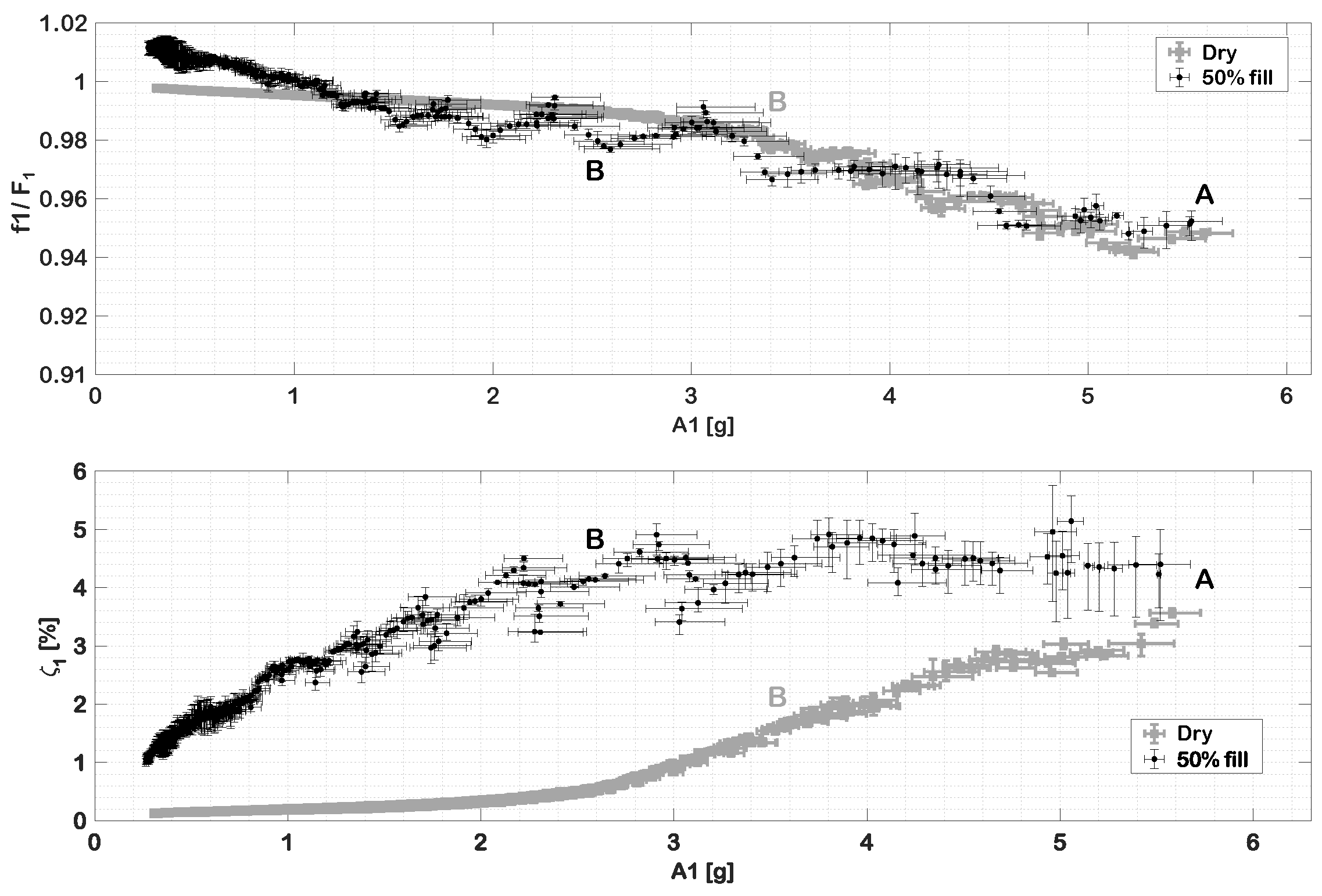
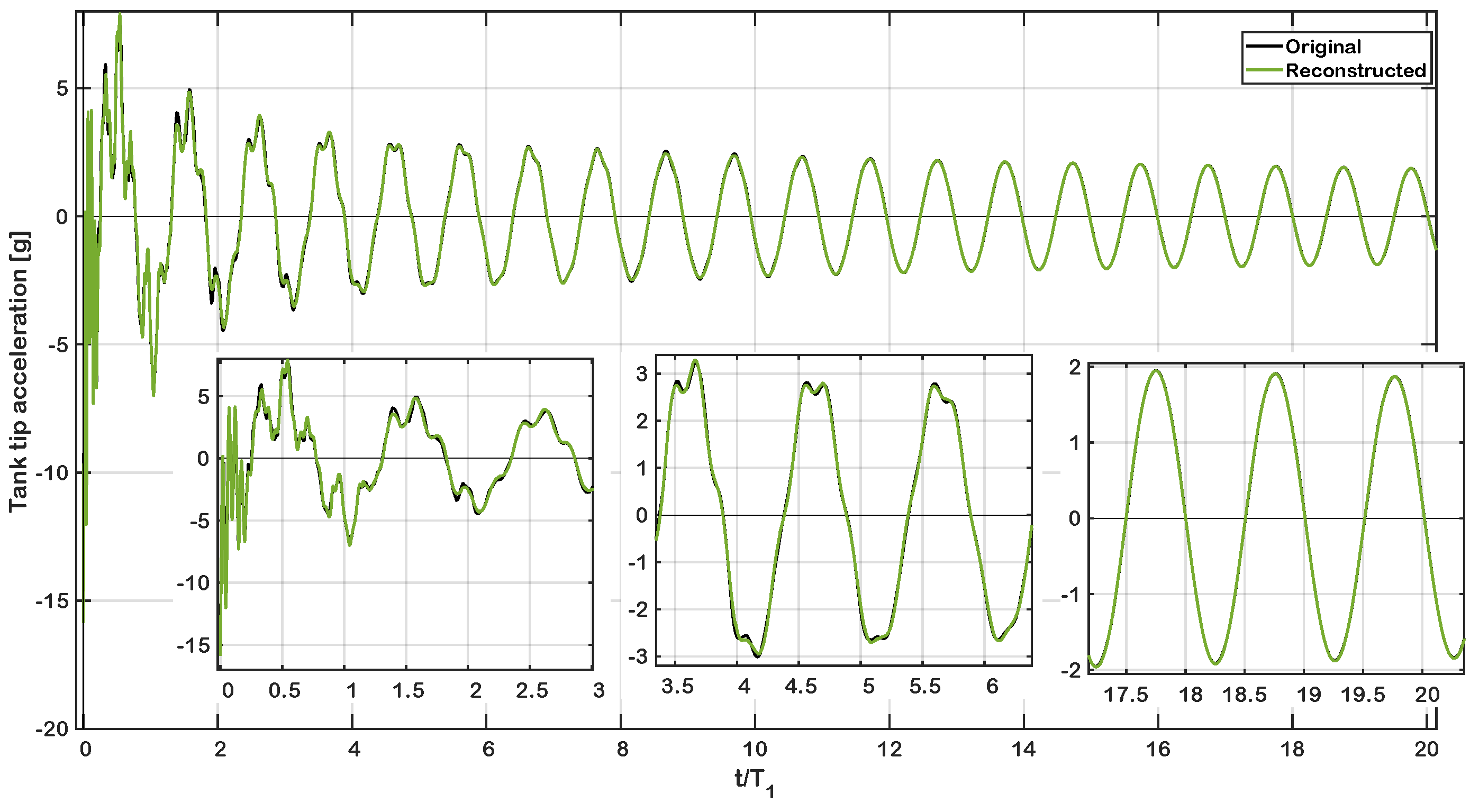
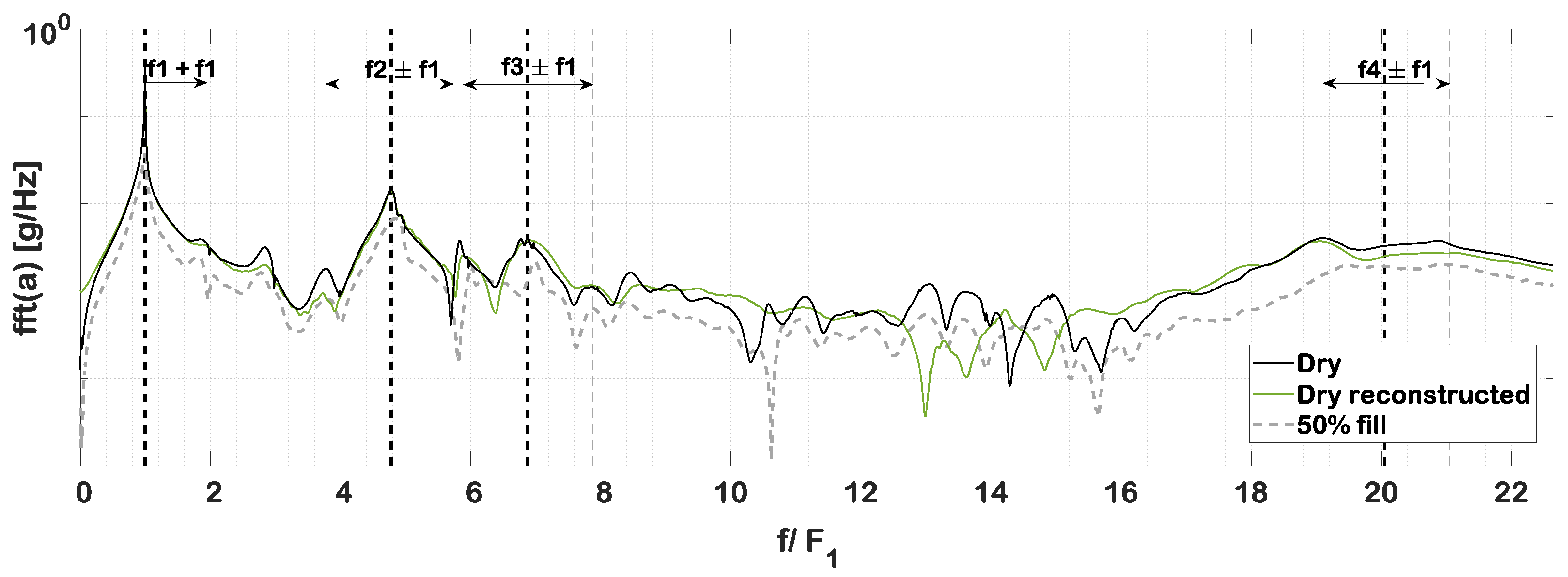
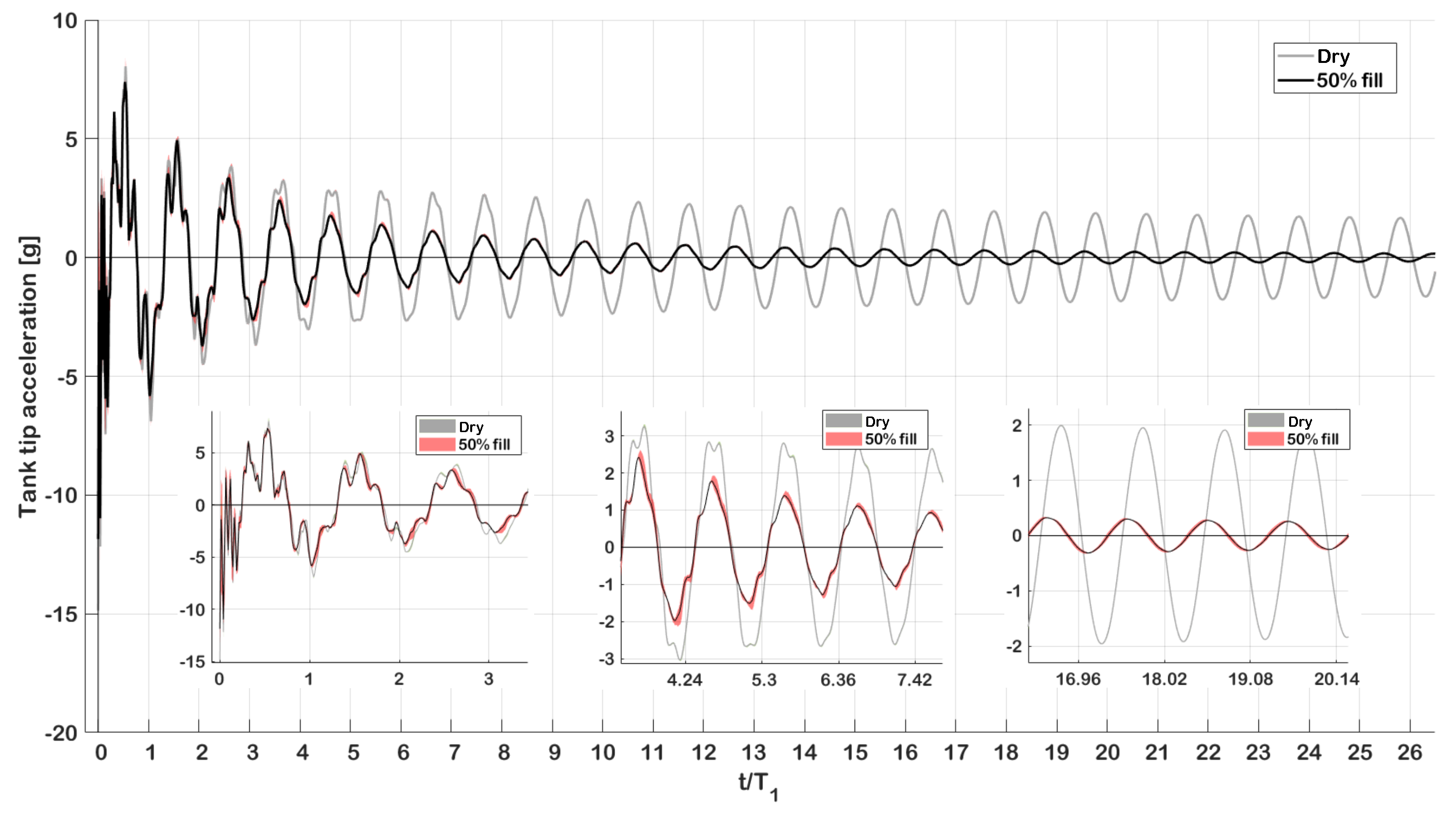
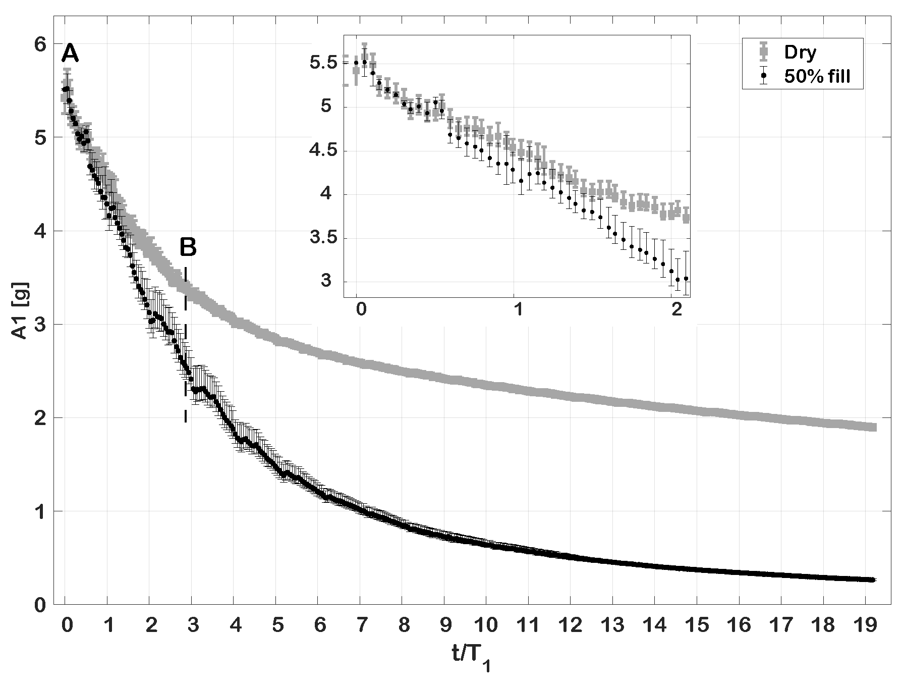
3.1. Large Amplitude Vibrations of the Dry System

It is instructive to begin the analysis by assessing the frequency–amplitude characteristic of the transient response of the dry structure. Figure 9 shows the amplitude–frequency characteristic of the vertical acceleration response at the tip of the tank computed over the first 20 periods of motion T1, after the step release with a tip deformation of 2.7% of the semispan. The same characteristic is included for the wet case for reference. The frequency components that are seen to have the most significant contribution to the transient signal are found in the vicinity of the normal modes corresponding to the first two out-plane bending modes (F1 and F2), first torsional mode F3 and a higher-order out-plane bending mode F4. These first four response components, selected by observing the amplitude of their contribution, are thus considered in the system identification process, and the corresponding frequency peaks identified in Figure 9 are named $f_1$ to $f_4$. Another significant feature that can be observed in Figure 9 is the evidence of sidebands appearing due to the nonlinear geometric effects that manifest themselves as additional amplitude peaks, specifically at the frequencies offset by integer multiples of one or multiple principal frequency components. In this case, evidence of the F1 sidebands is immediately seen, as indicated by the amplitude peaks marked by the dashed vertical lines. Similar effects were observed in previous nonlinear studies [27]. The awareness of their presence in the shown frequency–response characteristics will be useful in the subsequent detailed analysis of the fitted response.

While the detailed analysis of the dry system will mainly be conducted in conjunction with the wet system, consideration is also given here to the robustness of the NLS procedure introduced in Section 2 when applied to this data set. As shown in Figure 1, there are three accelerometers distributed across the length of the fuel tank. The NLS procedure is applied to the three accelerometer signals repeatedly for all three test realisations. Figure 10 shows a summary of the results that were obtained, namely the identified amplitude of component 1 $A_1$, frequency $f_1$ (in Equation (1), $f_j={\omega }_j/\left(2\pi \right)$) and damping ratio ${\zeta }_1$ expressed as the percentage of critical damping. The mean values among the three repetitions are shown, together with the vertical bars showing minimum/maximum deviations.

Considering that the first component of the signal is dominated by the first modal contribution, the sensor-specific amplitude $A_1$ increases in value from the tank root to the tank tip, as expected. Furthermore, the identified frequency and damping ratio (middle and bottom of Figure 10) show consistent values regardless of which accelerometer is used. The error bars decrease in size from tank root to tip as the signal-to-noise ratio increases. For the frequency component dominated by the first bending mode, it would be expected to find the same damping and frequency characteristics regardless of the accelerometer position across the tank, and this is indeed the case. The results demonstrated here are mutually consistent and indicate the robustness of the proposed identification method. Similar results were observed for the other frequency components.

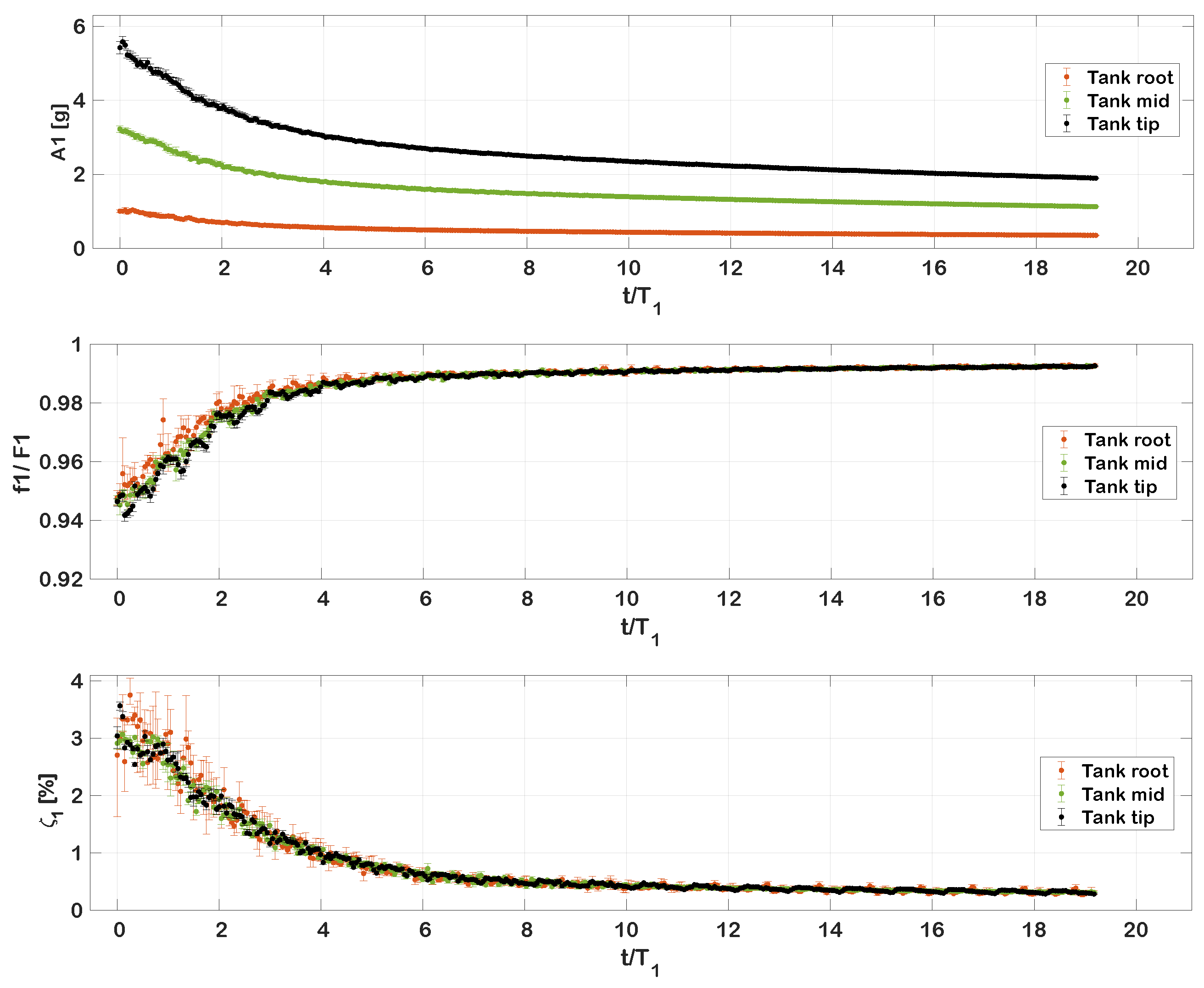
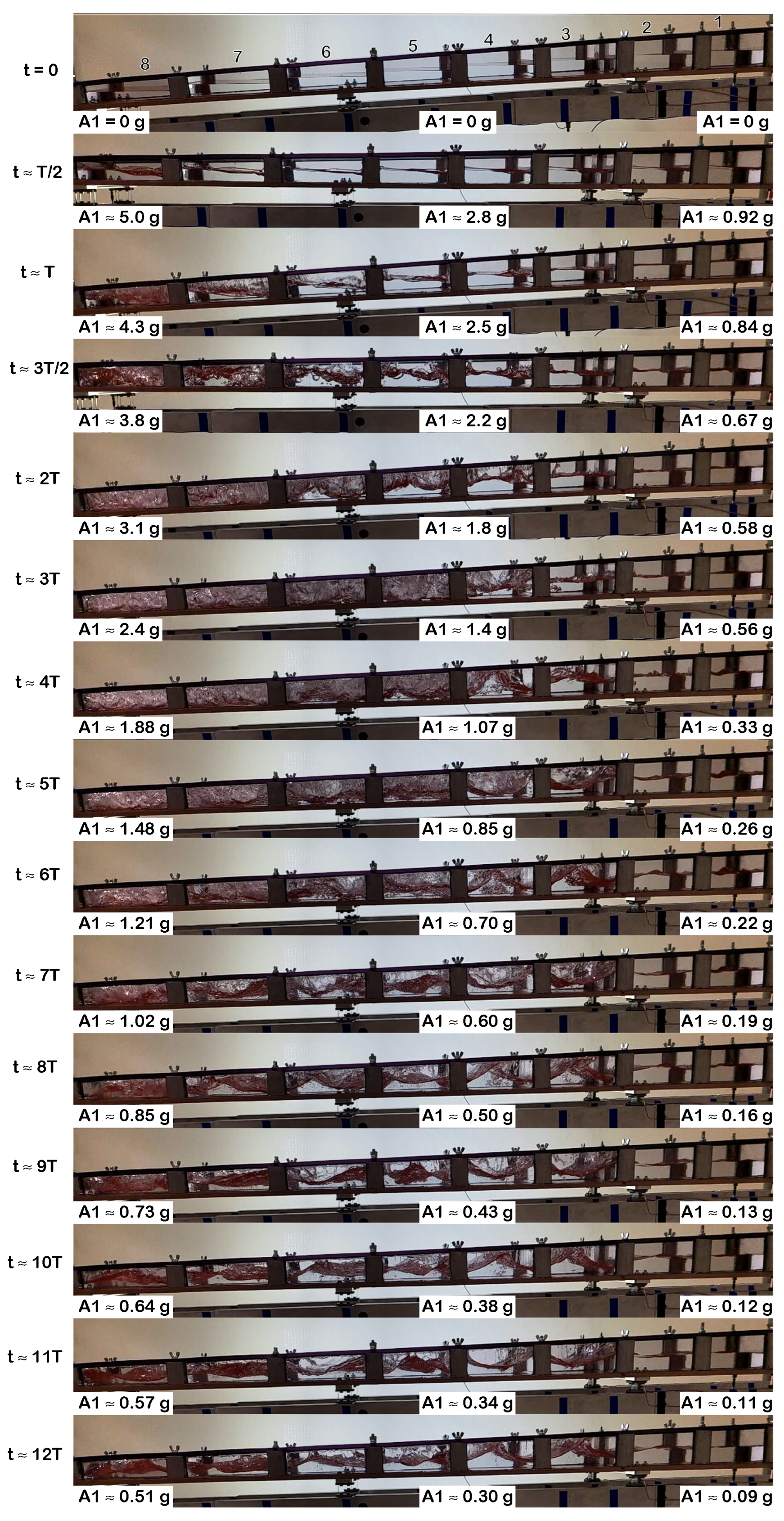
3.2. Large Amplitude Vibrations of the Wet System

For the wet analysis, the 50% filling level case was considered with the solid-section baffles. An initial overview of the differences between the dry and wet systems can be seen by inspecting the tank tip acceleration versus time for the two cases. These results are shown in Figure 11, where the time parameter was normalised by $T_1$. The mean values among the three repetitions are shown with the black curves, and the red/grey bands indicate the minimum and maximum acceleration values. Insets are included showing the detailed views at the selected times. The differences between the dry and wet cases in the first part of the transient are not noticeable. When the response progresses, the amplitude of the wet system drops faster as a first indication of the induced damping effects due to sloshing. Similar trends were noted in a simpler single degree of freedom transient sloshing tests [5]. There are also multiple frequency components noticeable immediately following the step release event, which decay at rates that are different between the dry and wet cases until the point when only the first frequency component is observable. Small phase shifts, which are indicative of the frequency differences, can also be observed when comparing the dry and wet systems. These aspects can be investigated further by decomposing the signal into its components using the NLS procedure.

Figure 12 and Figure 13 show the amplitudes, frequencies and damping ratios for the acceleration component corresponding to the first bending mode. Since the damping ratios for the wet and dry cases are different, the same acceleration values will be reached at different times, so the frequency and damping values are shown as a function of the component amplitude for comparison purposes. The tank tip acceleration across the three repetitions was used for this analysis, the markers and error bars having the same significance as before.

Starting with the second half of the first period of motion, a distinct drop of component 1 acceleration amplitude can be seen in Figure 12 for the wet case when compared to the dry case. It is interesting that this is not immediately obvious by inspecting the complete time series in Figure 11, the reason being that component 1 of the signal conveys only fractional information about the overall motion characteristics in the first cycle of motion (5.5 g of the 15 g peak acceleration). Other frequency components of the signal are thus seen to be dominant in the first part of the transient response. An initial half-period delay is noticeable for the wet case A1 amplitude to deviate and decrease below the dry response. This can be understood by studying these trends in conjunction with the liquid movement (this analysis will be conducted in Section 4). The differences in the amplitude components increase substantially afterwards. This is indicative of significant sloshing-induced dissipative effects influencing the first out-of-plane bending response component associated with mode F1. Two points of interest are also emphasised in Figure 12 and Figure 13: point A represents the step release event, and point B represents the point in time when the wet system reaches $A_1=2.5$ g.

The frequency variation trends are similar between the two cases, as seen at the top in Figure 13. Both vertical and horizontal error bars are now included, as there are small variations in both amplitude and frequency/damping among the three repetitions. The system starts with a frequency that steadily increases with the decreasing acceleration (and displacement) amplitude together with the substantial decrease in damping ratio and some possible other phenomena (e.g., structural nonlinearity, added mass effect due to the absence of in-vacuo conditions). In the bottom part of the same figure, the damping ratio of component 1 is shown as a function of the acceleration amplitude too. It is interesting to first note that significant differences in ${\zeta }_1$ are seen starting with the very first data point, unlike the amplitudes $A1$. The reason for this is that, in the system identification procedure, $A_j$ represents the amplitude at the beginning of the time bin, while ${\zeta }_j$ is characteristic of the entire two-period bin. While the amplitude $A1$ indeed does not change substantially in the first half-cycle of the motion, the damping ratio encapsulates information from the later times as well, where the liquid does have an effect. Since it was found that at least two periods of motion must be considered in order to reliably identify the time-localised damping measure of the first frequency component, this behaviour is a natural consequence of this type of analysis.

Point B in Figure 13 has a different position in the dry and wet cases since the different decay rates imply the reach of distinct amplitudes at the same time instant. In the 50% fill case, between points A and B, ${\zeta }_1$ occupies a relatively narrow region, while after point B it decreases with a near-linear trend. Similar damping trends were observed in 1DOF experiments [5], with regions of almost constant damping ratio characterising the violent vertical sloshing region denoted as R1. Single degree of freedom experiments also indicated that the damping ratio starts to decrease at even larger amplitudes of motion [6]. The same phenomenon will be investigated here using the numerical model that was developed based on the 1DOF experiments.

A modulation effect can also be seen in all three identified quantities—amplitude, frequency and damping, shown in Figure 10, Figure 12 and Figure 13. The identified modulation frequency is f1, and it appears to be more pronounced in the wet case. This effect is a manifestation of the internal nonlinear dynamics, which was already observed in the form of the frequency sidebands shown in Figure 9. Owing to its presence with the differing intensities between the dry and wet cases, this effect is influenced by both structural and fluid–structure nonlinear interactions.

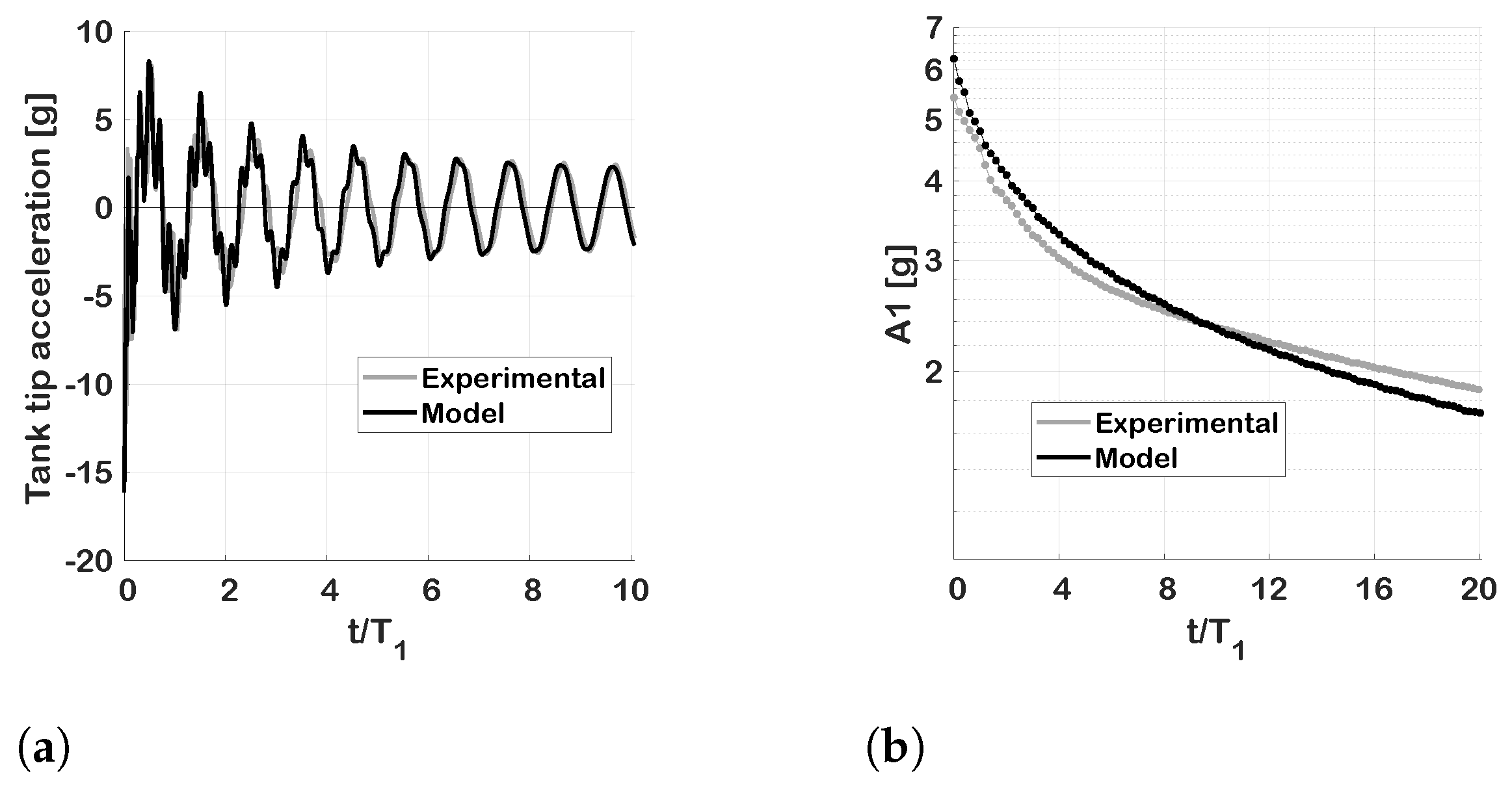
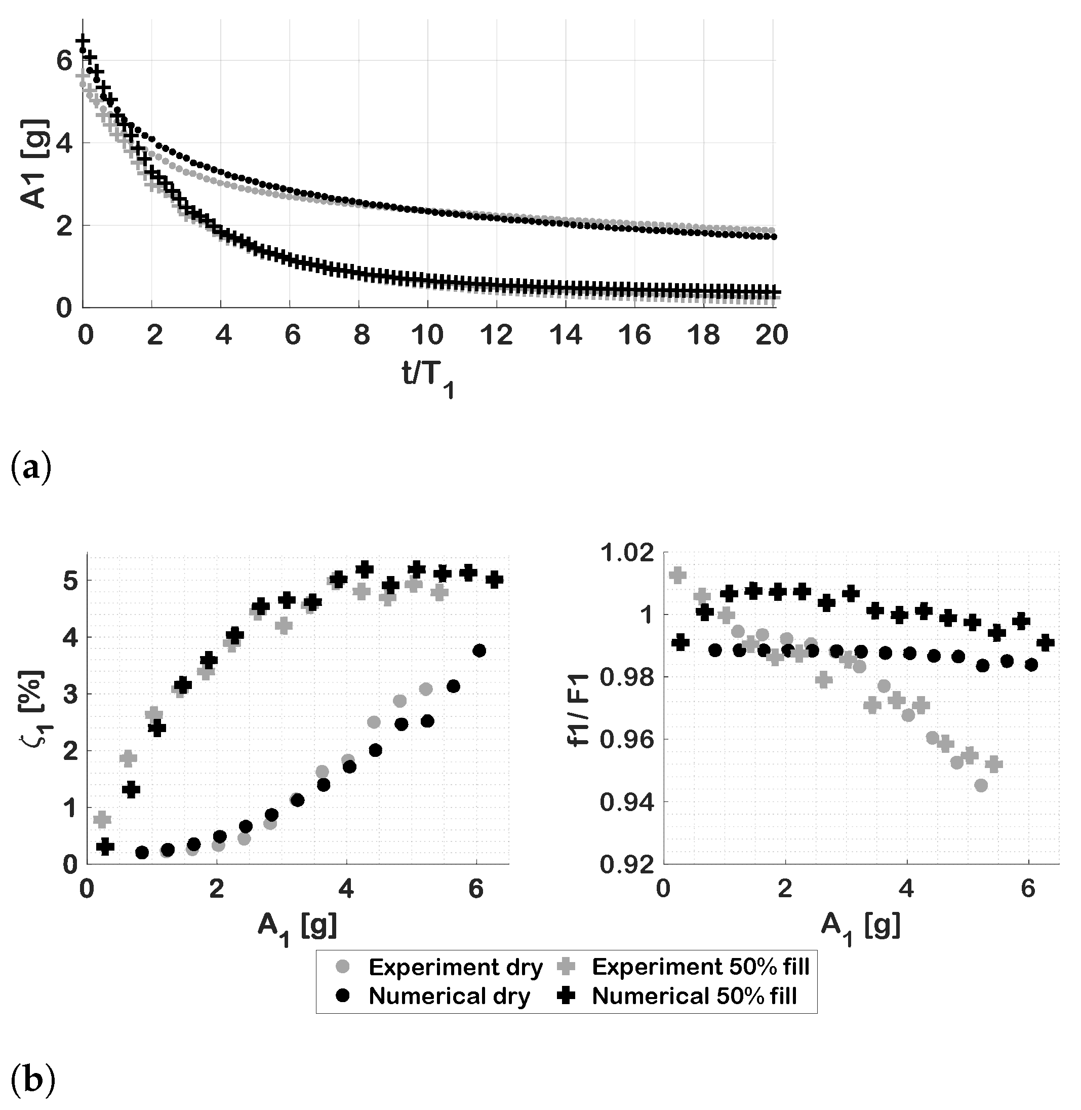
3.3. Numerical Results

Similarly to the experimental study, the structural model was loaded downward and released. Following this event, the structure vibrates freely and decays according to its dry damping and interaction with the fluid force model. As described in Section 2, the sloshing force acts on each tank cell depending on the local instantaneous displacement and velocity. Figure 14 shows the 7.3 Hz interpolated sloshing force map (surrogate model) and the trajectory of the recovered sloshing force in the displacement-velocity domain during the transient decay of tank cell number 8. The starting value is at the maximum displacement and 0 velocity, after which the system starts decaying in the clockwise direction. In various parts of the tank cycle, the liquid acts against the tank with different intensities. The steady-state hysteresis cycles that result from this interaction were studied in-depth in [7], and the collection of such cycles for multiple amplitudes of excitation determine the sloshing force magnitude in the different parts of the map shown in Figure 14. The colour map in Figure 14 also indicates that the sloshing liquid maximises the sloshing force in the vicinity of extreme $y/h$ values, with phasing between it and the tank velocity depending on the amplitude and frequency of excitation, consistent with previous observations [7]. Note that the $F_s$ values shown here are adjusted with the help of the force smoothing function during the first part of the transient response in order to take into account the region where the sloshing is initially formed (see Section 2, Figure 8).

Let us consider the comparison between the properties of the first bending component identified experimentally and those found using the numerical model. Figure 15 shows the evolution of the three response characteristics of the first signal component: amplitude versus time (upper side), damping ratio versus amplitude (left) and frequency versus amplitude (right), where these are given for the numerical and experimental realisation of the dry and wet cases. In order to facilitate the comparison of all data in one graph, a reduction in the data was made by averaging the acceleration-dependent quantities (e.g., the experimental data shown in Figure 13) inside bins of length 0.3 g. The mean values inside each bin are shown in Figure 15.

The numerical prediction of the variation of tank tip acceleration $A1(t/T1)$ agrees very well with the experimental data. There is a difference in the initial acceleration, even though the same initial displacement was used and the first bending frequency is the same. An initial assessment of the structural model under the transient conditions with geometrical nonlinearities included (Nastran SOL400) has shown that a reduction in the peak accelerations similar to what is seen in Figure 15 is obtained, suggesting that this difference has its source in the use of the linear modal model. While this difference does not impede other comparisons or validity of the numerical simulations, the adoption of a nonlinear model in the future might provide an improved acceleration amplitude match for cases similar to the one analysed here.

The dry and wet damping ratio is shown as well in comparison in Figure 15. The numerical nonlinear dry damping was tuned based on the experimental data using the model described in Section 2, with the resulting damping model parameters shown in Table 2. There is a very good agreement in wet case damping ratios throughout the full acceleration amplitude range. At high amplitudes, the damping of the system is dominated by the structural effects and the sloshing force smoothing function (Equation (10)) improves the agreement in the 4–6 g range. At lower amplitudes, i.e., the $A1<2.5$ g region, where lower amplitude sloshing patterns dominated by different sloshing modes define the liquid motion, the induced damping effects are significantly influenced by parametric excitation of the liquid. This will be discussed further in Section 4. The frequencies, shown on the right-hand side, indicate slightly different trends with respect to the acceleration amplitude. Following the step release, the experimental case indicates a frequency increase towards the first bending mode frequency in both the dry and wet cases. The numerical model shows an approximately constant frequency trend with slightly higher values in the wet case. It is interesting to note that the 50% wet case numerical frequencies converge towards the dry values when the acceleration drops below 1 g; that is, the region where the liquid is not substantially vertically excited anymore, and the sloshing force drops considerably. Overall, since the model versus experiment frequency differences are observed in both wet and dry cases, this suggests that they may be attributable to errors in the linear approximation of the structural model or unaccounted dynamics. In the present study, however, such considerations do not significantly influence the results, and it captures the main features observed experimentally.

4. Discussion

The liquid sloshing-induced trends observed in Section 3 can be better understood in conjunction with an analysis based on the visually observed sloshing patterns. As explained in Section 2, two high frame rate video snapshots were used to observe the liquid sloshing from the side and top of the tank. Examples of video frames from one 50% filling level representative test are shown in Figure 16 at the selected time instances expressed as multiples of the period of oscillation of the first bending mode. Three guiding acceleration values are also reported for each snapshot, indicating the first component’s amplitude at the corresponding location using the three tank accelerometers, as shown in Figure 1 (root, mid and tip). The tank is oriented here, with its outboard end towards the left.

It was noted, in relation to Figure 12 and Figure 13, that the amplitude $A1$ is the same for the dry and wet cases in the first half-period of the transient motion. Figure 16 now offers a visual interpretation of this result. The liquid starts from a standstill configuration at t = 0, and then, following the release event, it starts moving together with the structure upwards. Only between t = T/2 and t = T does the liquid start moving substantially upwards relative to the tank and starts impacting the ceiling of the tank. After this, the sloshing fully develops across all spanwise stations. The sloshing force acting on the tank was, in the past studies, isolated and shown to be correlated with the movement of the liquid relative to the tank in harmonically-excited systems [7]. A single degree-of-freedom system with the sloshing liquid undergoing a free transient vibration exhibits qualitatively and quantitatively different behaviours depending on the combined fluid–structure response characteristics. It was shown in [5] that the following vertical sloshing regimes and corresponding damping regions can be identified: R1—the most dissipative regime, characterised by the violent vertical sloshing with regular impacts between the liquid and the top/ceiling of the tank and R2—the region characterised by the well-defined fluid motion in one of its sloshing modal patterns with possible intermittent impacts with the top of the tank characterised by the dissipation rates notably higher than those of the underlying dry system. A transition region R2&R1 was also shown in [7], where both effects contribute depending on the amplitude of excitation. In regard to the vertical accelerations for these regimes, it was generally observed that at least 1g is needed to excite significant free-surface motion such that substantial and repeated impacts with the tank ceiling occur. Depending on the tank geometry, liquid sloshing modes can be excited at lower amplitudes as well, promoting more impacts with the top of the tank and thus more energy dissipation. All of these phenomena can be observed in the present case as well.

The peak accelerations of component 1 at the root-end of the tank do not exceed 1 g. Small surface ripples in cells 1 and 2 are seen to develop gradually, but their amplitude is likely not large enough to contribute to any substantial dissipation in the system. There is a noticeable difference between cells 2 and 3 in what concerns the observed sloshing patterns since the cell geometry changes substantially as well (see bottom section of Figure 1 and also Figure 17 showing the geometry-dependent first few sloshing frequencies in each tank cell). Moving towards the middle section of the tank, cells 3 and 4, vertical accelerations of up to 3.3 g are reached there. After approximately two initial periods of motion, the sloshing in these cells develops to start hitting the top of the tank. Liquid motions are dominated by the (2,0) sloshing mode (mode shape with two nodes) at a frequency of $F1/2$, as can be seen from the near-periodicity of the sloshing pattern in cells 3 and 4 corresponding to the two full tank periods. Note that each sloshing mode depends on the tank geometry and filling level, and the mode shape (m,n) is characterised by m nodes in the spanwise direction and n nodes in the chordwise direction [28].

The vertical acceleration gradient increases further towards the tip-end of the tank (left-hand side in Figure 16), where the maximum A1 accelerations of 5.5 g are reached. This gradient causes the liquid sloshing motion to be increasingly more violent as we move from cells 5 to 8. This violent vertical behaviour is observed up to t = 9 T in cell 8 followed by only occasional roof impacts afterwards. These motions are typical of the most dissipative region R1. Furthermore, since these violent sloshing patterns are localised predominantly outboard, the developed sloshing force has a larger moment arm relative to the root, maximising thus the dissipative influence of the sloshing liquid.

The numerical results presented in Section 3 confirm the experimentally-observed damping trends, and the high amplitude behaviour was shown to be modelled well when a sloshing smoothing function is considered in the first part of the transient (see Section 3, Figure 15). Shifting focus on the lower acceleration amplitude range, past point B in Figure 12 and Figure 13, it was mentioned in Section 2 that the choice of the surrogate model’s frequency is not straightforward. The reason behind this is that different tank geometries at different scales can excite different sloshing patterns. Figure 17 shows the spanwise variation of the three sloshing mode frequencies (for modes (2,0), (2,1) and (1,2)) depending on tank cell geometry. For example, Figure 18 shows the high amplitude sloshing patterns developed from the first symmetric sloshing mode (2,0). Since the tank width (dimension in the chordwise direction) is variable, the sloshing frequencies were approximated considering an average tank width for each cell. The direction of excitation is significantly vertical, and the sloshing patterns will be excited when the frequency of excitation (F1 in this case) is double the sloshing modal frequency. This parametric excitation regime generates Faraday waves [28]. Such effects were extensively studied before in the controlled high-amplitude vertical sloshing experiments and were shown to be responsible for energy dissipation [5,7]. As seen in Figure 17, the sloshing mode (2,0) has its frequency in the vicinity of one-half of the first bending mode frequency of the MiniWot demonstrator for most of the tank cells. Furthermore, especially in the cells closer to the tip of the wing model (6,7,8), there are two additional modes (2,1) and (1,2) that may be excited. This suggests that in-plane sloshing influences can be expected at the tip of the wing. Referring to Figure 16, this behaviour can indeed be observed in the recorded footage. This discussion shows that the insights based on the linear modal analysis can still be used to support the analysis of these highly nonlinear and transient sloshing regimes.

Figure 18 evidences a similarity between the sloshing patterns based on which the surrogate model was generated (Section 2) and those observed in the MiniWoT experiments. On the left-hand side, the averaged location of the sloshing surface under harmonic excitation can be seen for the 8.3 Hz frequency of excitation. This sloshing pattern involves energy-dissipative liquid impacts on the top of the tank, with substantial influences on the sloshing mode shape (2,0). On the right-hand side, similar patterns are observed in MiniWoT tank cells where the local Froude number ($Fr=\sqrt{A_1/g}$) is similar at approximately 1.17. Since these sloshing patterns are highly dissipative, accounting for their influence in the reduced-order sloshing model was found to be essential in order to model the induced damping effects at lower acceleration amplitudes (i.e., the $A_1<2.5 g$ region in Figure 15) appropriately.

The above insights lead to the following main observations and motivate future research directions:

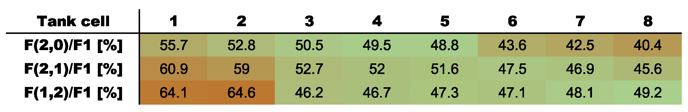
• The spanwise location of the fuel influences the vertical sloshing regimes. Previous single degree-of-freedom studies indicate substantial sloshing-induced damping effects that depend on the sloshing regime [5,7]. There is thus an indication that depending on the available amounts of fuel, the net damping following the excitation similar to the step release (such as a discrete gust) may be increased by moving the liquid to the specific spanwise positions, taking into account the filling level as well. Supplementary investigations are planned in order to further assess such effects.
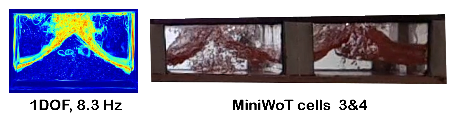
• Liquid sloshing patterns dominated by different sloshing modes are prominent at different spanwise locations and persistent even at the lowest amplitudes of excitation. Such sloshing modes are highly dependent on the geometry of the tank and filling level, and they have previously been observed to add substantial additional damping at lower amplitudes by promoting liquid impacts with the top of the tank. Therefore, there exists the possibility that the geometry of the fuel tank could be tailored to promote such sloshing patterns and, hence, achieve an increased sloshing-induced damping.

5. Conclusions

A scaled research prototype model was presented, representative of the static and dynamic behaviour and the geometry of a commercial aircraft wing. The experimental rig was equipped with a transparent fuel tank and was loaded vertically and released, aiming to achieve conditions similar to the loading experienced by the aircraft wings during the discrete gusts encounters. A numerical model developed based on 1DOF data was presented and employed for the same cases studied experimentally. The focus of this work was placed on the comparative analysis between the 50% filling level case using tap water as the working liquid and the dry case with the added equivalent liquid mass. The freely decaying response of the system was measured at multiple points using accelerometers, and three measurement points across the fuel tank were used for the analysis.

Evidence of substantial additional energy dissipation was shown in the first out-plane bending mode. Substantial increases in the damping ratio and corresponding decreases in amplitude were evident, starting with the second half of the first cycle of motion and further developing depending on the spanwise location. Correlation with previously obtained results for 1DOF vertically sloshing systems, as well as video captures from the side of the fuel tank, indicated links between liquid sloshing patterns at various vertical acceleration amplitudes and the induced damping effects. A numerical model was presented based on a modal representation of the dry structure with calibrated nonlinear dry damping, coupled with a surrogate fluid model interpolated from experimental 1DOF data. The model was shown to predict the induced damping effects at all amplitudes, provided that corrections are made for the initial sloshing development region. The low amplitude regimes were modelled correctly if similar sloshing patterns that promote liquid-tank roof slamming were considered.

The results shown in this work represent an initial assessment of some of the sloshing tests conducted on the MiniWoT specimen and indicate important liquid sloshing-induced effects manifested in the first bending component. The addition of 50% liquid inside the system led to significantly higher energy dissipation rates. The tests presented here also indicate and motivate planned future directions of study, such as the influence of the spanwise position of the liquid, filling level and tank geometry.

References

1. EASA. Certification Specifications and Acceptable Means of Compliance for Large Aeroplanes (CS-25) Amendment 27; Technical Report AMC 25.341 Gust and Continuous Turbulence Design Criteria, Section 6—Aeroplane Modelling Considerations; European Union Safety Aviation Agency (EASA): Cologne, Germany, 24 November 2021.
2. Stodieck, O.; Cooper, J.E.; Weaver, P.M.; Kealy, P. Aeroelastic Tailoring of a Representative Wing Box Using Tow-Steered Composites. AIAA J. 2017, 55, 1425–1439. [Google Scholar] [CrossRef] [Green Version]
3. Castrichini, A.; Siddaramaiah, V.H.; Calderon, D.; Cooper, J.; Wilson, T.; Lemmens, Y. Preliminary investigation of use of flexible folding wing tips for static and dynamic load alleviation. Aeronaut. J. 2017, 121, 73–94. [Google Scholar] [CrossRef] [Green Version]
4. Constantin, L.; De Courcy, J.J.; Titurus, B.; Rendall, T.; Cooper, J.E.; Gambioli, F. Initial Experimental Analysis of Damping due to Liquid Sloshing in a Scaled Aircraft Wing Model. In Proceedings of the International Forum on Aeroelasticity and Structural Dynamics IFASD 2022, Madrid, Spain, 13–17 June 2022. [Google Scholar]
5. Constantin, L.; De Courcy, J.; Titurus, B.; Rendall, T.; Cooper, J. Analysis of damping from vertical sloshing in a SDOF system. Mech. Syst. Signal Process. 2021, 152, 107452. [Google Scholar] [CrossRef]
6. Martinez-Carrascal, J.; González-Gutiérrez, L. Experimental study of the liquid damping effects on a SDOF vertical sloshing tank. J. Fluids Struct. 2021, 100, 103172. [Google Scholar] [CrossRef]
7. Constantin, L.; De Courcy, J.; Titurus, B.; Rendall, T.; Cooper, J. Sloshing induced damping across Froude numbers in a harmonically vertically excited system. J. Sound Vib. 2021, 510, 116302. [Google Scholar] [CrossRef]
8. Saltari, F.; Pizzoli, M.; Coppotelli, G.; Gambioli, F.; Cooper, J.E.; Mastroddi, F. Experimental characterisation of sloshing tank dissipative behaviour in vertical harmonic excitation. J. Fluids Struct. 2022, 109, 103478. [Google Scholar] [CrossRef]
9. Calderon-Sanchez, J.; Martinez-Carrascal, J.; Gonzalez-Gutierrez, L.M.; Colagrossi, A. A global analysis of a coupled violent vertical sloshing problem using an SPH methodology. Eng. Appl. Comput. Fluid Mech. 2021, 15, 865–888. [Google Scholar] [CrossRef]
10. Wright, M.D.; Gambioli, F.; Malan, A.G. CFD Based Non-Dimensional Characterization of Energy Dissipation Due to Verticle Slosh. Appl. Sci. 2021, 11, 10401. [Google Scholar] [CrossRef]
11. Saltari, F.; Pizzoli, M.; Gambioli, F.; Jetzschmann, C.; Mastroddi, F. Sloshing reduced-order model based on neural networks for aeroelastic analyses. Aerosp. Sci. Technol. 2022, 127, 107708. [Google Scholar] [CrossRef]
12. Titurus, B.; Cooper, J.E.; Saltari, F.; Mastroddi, F.; Gambioli, F. Analysis of a Sloshing Beam Experiment. In Proceedings of the International Forum on Aeroelasticity and Structural Dynamics, Savannah, GA, USA, 9–13 June 2019. [Google Scholar]
13. Constantin, L.; De Courcy, J.J.; Titurus, B.; Rendall, T.; Cooper, J.E. Design and GVT of a dynamically scaled wing structure for fuel sloshing investigations. In Proceedings of the AIAA SCITECH 2022 Forum, San Diego, CA, USA, 3–7 January 2022. [Google Scholar] [CrossRef]
14. Billings, S.A. Nonlinear System Identification: NARMAX Methods in the Time, Frequency, and Spatio-Temporal Domains; John Wiley & Sons: Hoboken, NJ, USA, 2013. [Google Scholar]
15. Billings, S.A.; Voon, W.S.F. Piecewise linear identification of non-linear systems. Int. J. Control 1987, 46, 215–235. [Google Scholar] [CrossRef]
16. MSC Software. NASA STRuctrual ANalysis (NASTRAN) 2018. Available online: https://www.mscsoftware.com/product/msc-nastran (accessed on 1 August 2022).
17. MSC Software. MSC Patran 2018. Available online: https://www.mscsoftware.com/product/patran (accessed on 1 August 2022).
18. Cveticanin, L. Oscillators with nonlinear elastic and damping forces. Comput. Math. Appl. 2011, 62, 1745–1757. [Google Scholar] [CrossRef] [Green Version]
19. Cveticanin, L.; Kalamiyazdi, M.; Askari, H.; Saadatnia, Z. Vibration of a two-mass system with non-integer order nonlinear connection. Mech. Res. Commun. 2012, 43, 22–28. [Google Scholar] [CrossRef]
20. Shampine, L.F.; Reichelt, M.W. The matlab ode suite. SIAM J. Sci. Comput. 1997, 18, 1–22. [Google Scholar] [CrossRef] [Green Version]
21. Dodge, F. The New “Dynamic Behavior of Liquids in Moving Containers”; Technical Report; Southwest Research Institute: San Antonio, TX, USA, 2000. [Google Scholar]
22. Farid, M.; Gendelman, O. Response regimes in equivalent mechanical model of moderately nonlinear liquid sloshing. Nonlinear Dyn. 2018, 92, 1517–1538. [Google Scholar] [CrossRef] [Green Version]
23. Pizzoli, M.; Saltari, F.; Mastroddi, F.; Martinez-Carrascal, J.; González-Gutiérrez, L.M. Nonlinear reduced-order model for vertical sloshing by employing neural networks. Nonlinear Dyn. 2022, 107, 1469–1478. [Google Scholar] [CrossRef]
24. Pizzoli, M.; Saltari, F.; Coppotelli, G.; Mastroddi, F. Experimental Validation of Neural-Network-Based Nonlinear Reduced-Order Model for Vertical Sloshing. In Proceedings of the AIAA Scitech 2022 Forum, San Diego, CA, USA, 3–7 January 2022; p. 1186. [Google Scholar]
25. Wendland, H. Scattered Data Approximation; Cambridge University Press: Cambridge, UK, 2004; Volume 17. [Google Scholar]
26. Saltari, F.; De Courcy, J.; Pizzoli, M.; Constantin, L.; Mastroddi, F.; Coppotelli, G.; Titurus, B.; Rendall, T.; Cooper, J.; Gambioli, F. Data driven and model-based vertical sloshing reduced order models for aeroelastic analysis. In Proceedings of the International Forum on Aeroelasticity and Structural Dynamics, Madrid, Spain, 13–17 June 2022. [Google Scholar]
27. Malatkar, P.; Nayfeh, A.H. On the Transfer of Energy between Widely Spaced Modes in Structures. Nonlinear Dyn. 2003, 31, 225–242. [Google Scholar] [CrossRef]
28. Ibrahim, R.A. Liquid Sloshing Dynamics: Theory and Applications; Cambridge University Press: Cambridge, UK, 2005. [Google Scholar]
Figure 1. MiniWoT scaled test specimen. Top figure: (1)—Cantilever to the strong wall connection, (2)—scaled structure model, (3)—scaled fuel tank model and (4)—loading points for step release tests. Bottom figure: instrumentation layout.
Applsci 12 07860 g001
Figure 2. Binning of the time data and NLS fitting procedure.
Applsci 12 07860 g002
Figure 3. Example of NLS identification result. Original signal is shown in black and the reconstructed signal using the fitted functions is shown in green.
Applsci 12 07860 g003
Figure 4. Example of residuals and summed squared residuals for the fitted functions shown in Figure 3: (a) residuals for the first bin; (b) summed squared residuals for all bins.
Applsci 12 07860 g004
Figure 5. MiniWoT finite element model overview.
Applsci 12 07860 g005
Figure 6. Tank tip acceleration comparison between experiment and model. Deflection at the tip of the wing is 2.7% of the semispan: (a) acceleration time series for the dry case; (b) amplitude of the first bending component versus time.
Applsci 12 07860 g006
Figure 7. Interpolated experimental response surfaces. Circular traces shown in the horizontal plane corresponding to the 3.3 Hz response surface.
Applsci 12 07860 g007
Figure 8. Sloshing force smoothing function used for the first part of the transient response.
Applsci 12 07860 g008
Figure 9. Frequency response function for the dry and wet systems. The NLS-identified dry system is shown in green for comparison.
Applsci 12 07860 g009
Figure 10. The amplitude, frequency and damping ratio of the first frequency component (component 1) of the acceleration time series measured throughout the fuel tank, dry case.
Applsci 12 07860 g010
Figure 11. Typical sloshing response of the MiniWoT structure, 50 % filling level case compared to dynamically equivalent dry case.
Applsci 12 07860 g011
Figure 12. Amplitude of component 1 vs. normalised time, 50% filling level case and dynamically equivalent dry case. Error bars show the variability between test repetitions.
Applsci 12 07860 g012
Figure 13. Component 1 frequencies and damping ratios vs. component 1 acceleration amplitude, 50% filling level and dynamically equivalent dry case. Error bars show the variability between test repetitions. The amplitude decays following the step release event at A.
Applsci 12 07860 g013
Figure 14. Interpolated sloshing force map and trajectory of sloshing force for tank cell 8.
Applsci 12 07860 g014
Figure 15. Comparison between experimental and numerical amplitude, frequency and damping ratio of the first bending component: (a) amplitude of first bending component versus time; (b) damping ratio and frequency versus amplitude.
Applsci 12 07860 g015
Figure 16. Selection of video segments for one representative 50% filling level test. Local acceleration for the first vibration component shown (left: tank tip).
Applsci 12 07860 g016
Figure 17. Estimation of sloshing mode frequencies for the 50% filling level case for each MiniWoT tank cell, shown as a percentage of F1. Values coloured by their proximity to 50%.
Applsci 12 07860 g017
Figure 18. Average liquid surface location in 1DOF harmonic excitation tests [7] (left) and MiniWoT cells 3&4 sloshing pattern (right).
Applsci 12 07860 g018