Determining the Dynamic Characteristics of a Multi-Story RC Building Located in Chile: A Comparison of the Results between the Nonparametric Spectral Analysis Method and the Parametric Stochastic Subspace Identification Method

Abstract

Estimating the dynamic characteristics of instrumented built structures from seismic vibration data collected from built civil structures is essential input information for structural model updating and assessing the health of structures. This study focuses on the earthquake acceleration time histories obtained from several events recorded during its construction phase by accelerometers placed throughout an office building located in Viña del Mar (Chile) to determine its modal features. To this end, the data obtained were analyzed to compare the building’s dynamic properties obtained with two different modal identification techniques. MATLAB programs were developed to implement both methods. The stochastic subspace identification technique for linear systems developed by van Overschee and de Moor was used to study the dynamic properties of the building. In contrast, the nonparametric method employed herein uses correlations and spectral analysis based on the Welch transform in the frequency domain. The investigation demonstrated that both methods identify similar frequencies and that the obtained translational mode shapes exhibit good agreement. Furthermore, the identified frequencies are congruent with the design frequencies.

1. Introduction

Chile is located along the Pacific Ring of Fire, which experiences large earthquakes on a frequently recurring basis. The deep subduction zone earthquake that occurred on 27 February 2010, exhibited a remarkably high magnitude of Mw 8.8 and lasted approximately 3 min. This event affected at least one-third of the nation, the longest country in the world, and released an energy equivalent to 11,780 Hiroshima bombs. Therefore, news of this event spread worldwide. The earthquake generated relatively few cases of structural failure. A study conducted by the Chilean Structural Engineers Association concluded that 11% of the infrastructure in the country’s capital city required major repairs to nonstructural elements; 3% presented minor or medium failures in the structure that could be repaired, and a mere 0.4% corresponded to severely damaged or collapsed structures that had to be demolished [1]. The low level of damage suffered by Chilean buildings in the face of such a strong earthquake, in comparison with that of structures in Christchurch, New Zealand, following the 2010 Canterbury earthquake or in Manabí, Ecuador, in response to the 2016 Ecuador earthquake, has intrigued the earthquake engineering community around the world.

Eleven years after the 2010 event, research on its effects on built civil infrastructure is still of great relevance, with studies being continuously performed to improve current structural design codes and thus ensure satisfactory structural performance [2,3]. In particular, Chile is seen as a natural laboratory that provides the national and international earthquake engineering communities with the opportunity to calibrate structural design standards and serves as a reference in the earthquake-resistant construction industry.

The earthquake-resistant design aims to ensure that structures can adequately resist seismic forces, limiting the seismic risk and guaranteeing peoples’ well-being. To this end, standards committees continue to propose design models or methodologies based on experiences such as those of Chile in 2010. Therefore, it is imperative to develop techniques that increase our knowledge and to evaluate the adequacy of proposed design methods through measurements. In this regard, monitoring large structures such as bridges, buildings, and dams is critical for calibrating the existing design methodologies and assessing their safety and health. Typical monitoring approaches for such structures are based on the analysis of either static strain or displacement data or discrete and continuous dynamic acceleration data gathered at specified points in the structures [4,5,6,7,8].

To obtain dynamically measured data, the proper monitoring of a structural system necessitates the collection of vast volumes of data over specified periods, from which mode shapes or other dynamic properties of the structures can be derived. Modal parameter changes in structures provide helpful information about the state of health of structural systems, provided that the dynamic features predicted in the design stage are affected by construction processes as well as seismic phenomena. The dynamic characteristics of structures can be derived either passively from ambient conditions [9] or actively by force excitations [10,11]. Then, modal parameters such as natural frequencies, damping factors, and mode shapes can be obtained based on response data. Thus, the structural properties can be estimated, and the performance and integrity of a structure can be assessed [12,13].

Modal analysis approaches yield essential information on the overall health of buildings. The process of determining the modal parameters of structures typically entails the deployment of accelerometers, gathering vibration data and using one of many analytic techniques. The accuracy of the data is based on not only the number, measurement sites, and resolution of the accelerometers but also the choice of a suitable analytic approach. In particular, the number and positions of sensors significantly impact the outcome. However, as buildings increase in size and become more complicated, the deployment of a slew of accelerometers becomes prohibitively expensive, especially about the number of sensors, the correct sensor placement, and the amount of gathered data (in terms of processing vast volumes of dynamic data), and the analytic technique [14,15].

Fang et al. [16] developed a method to extract the modal parameters of structures based on distributed measurements of dynamic strains using optical fiber sensors in a laboratory beam. The laboratory results indicated that the distributed vibration strain collected was sufficient for convergence. Hence, the first two mode shapes were accurately determined. The dynamic response characteristics of a 51-story building in downtown Los Angeles during the 2019 Mw 7.1 Ridgecrest, California, earthquake were identified from recorded response data, which was possible due to the consideration of other natural hazards, the use of system identification methods, the application of spectral analysis, and computing the coherence-phase angle spectrum [17]. The reinforced concrete (RC) building comprises a dual-core shear wall, perimeter columns, and post-tensioned flat slabs for approximately 80% of the floors. The recorded acceleration levels were trim (0.014 g at the foundation level and 0.069 g at the roof), and the maximum drift ratio computed from the recorded data was ~0.15%, so there were no reports of observed damage. Schanze et al. [18] compared and analyzed several models to study the effects of different underground story modeling methodologies using 11 aftershocks with different hypocenters and magnitudes recorded for a 16-story building office located in the city of Viña del Mar, Chile. The results revealed strong agreement between the model and the actual vibration data for the models considering horizontal springs attached to the retaining walls of the subterranean stories to account for the soil-structure interaction. Wu et al. [19] used a modified discrete-time Fourier transform combined with moving window technology in the time domain to examine the time-varying dynamic features of Shanghai Tower under the stimulation of normal wind and two subsequent typhoons. According to the authors, the findings can help with the wind-resistant design of significantly high-rise structures.

Currently, state-of-the-art modal analyses of already built structures indicate that there is more than one method with which the dynamic properties of buildings can be identified. These methods can be grouped into two main categories: parametric identification, which establishes a simplified mathematical model with which the measured and calculated responses can be compared, and nonparametric identification, which identifies the system by means of transformations, functions, and mathematical processes [20,21]. Some interesting works determining the dynamic response of heritage and modern structures with irregularities using system identification techniques can be consulted in the references [22,23,24,25]. In these works, different approaches are used to identify the main dynamic characteristics using accelerometers installed in the studied buildings. The general objective of this research is to compare both system identification philosophies, ascertain how compatible they are, and generate MATLAB code for both approaches that automate the analysis.

2. The Building, Temporary Instrumentation and Methodology

An instrumented structure should provide sufficient information to (a) reconstruct the response of the structure in sufficient detail to compare it with the responses predicted by mathematical models and with those observed in laboratories and, thereby improve the models; (b) make it possible to explain the reasons for any damage to the structure; and (c) facilitate decisions to retrofit/strengthen structural systems when warranted [26].

MATLAB codes were generated for each system identification philosophy based on a set of seismic event records. The building’s shaking responses to several aftershocks were recorded during the deployment of the array. Only four of the many response data are utilized in this study. The criterion used for selection was to consider earthquakes with the different magnitudes, hypocenter depths, and epicentral distances.

Table 1. List of seismic events recorded in the building (source: USGS).

Location	Date (MM-DD-YYYY)	Date	Depth (km)	Magnitude
Metropolitan Region	04-05-2010	03:32:12 UTC	58.6	4.5 (Mw (1))
Offshore Valparaíso	05-01-2010	14:41:08 UTC	35.0	5.0 (Mw)
Coquimbo	10-23-2010	01:38:14 UTC	44.0	5.2 (mb (2))
Araucania	01-02-2011	20:20:18 UTC	25.1	7.2 (Mi/Mwp (3))
Libertador O’Higgins	01-21-2011	15:36:11 UTC	18.2	5.0 (mb)
Offshore Maule	02-14-2011	03:40:10 UTC	25.4	6.6 (Mi/Mwp)

⁽¹⁾ M_w = Moment magnitude; ⁽²⁾ m_b = Body wave magnitude; ⁽³⁾ M_i/M_wp = Integrated p-wave.

lists the specifics seismic events considered herein.

2.1. Description of the Building and Sensor Layout

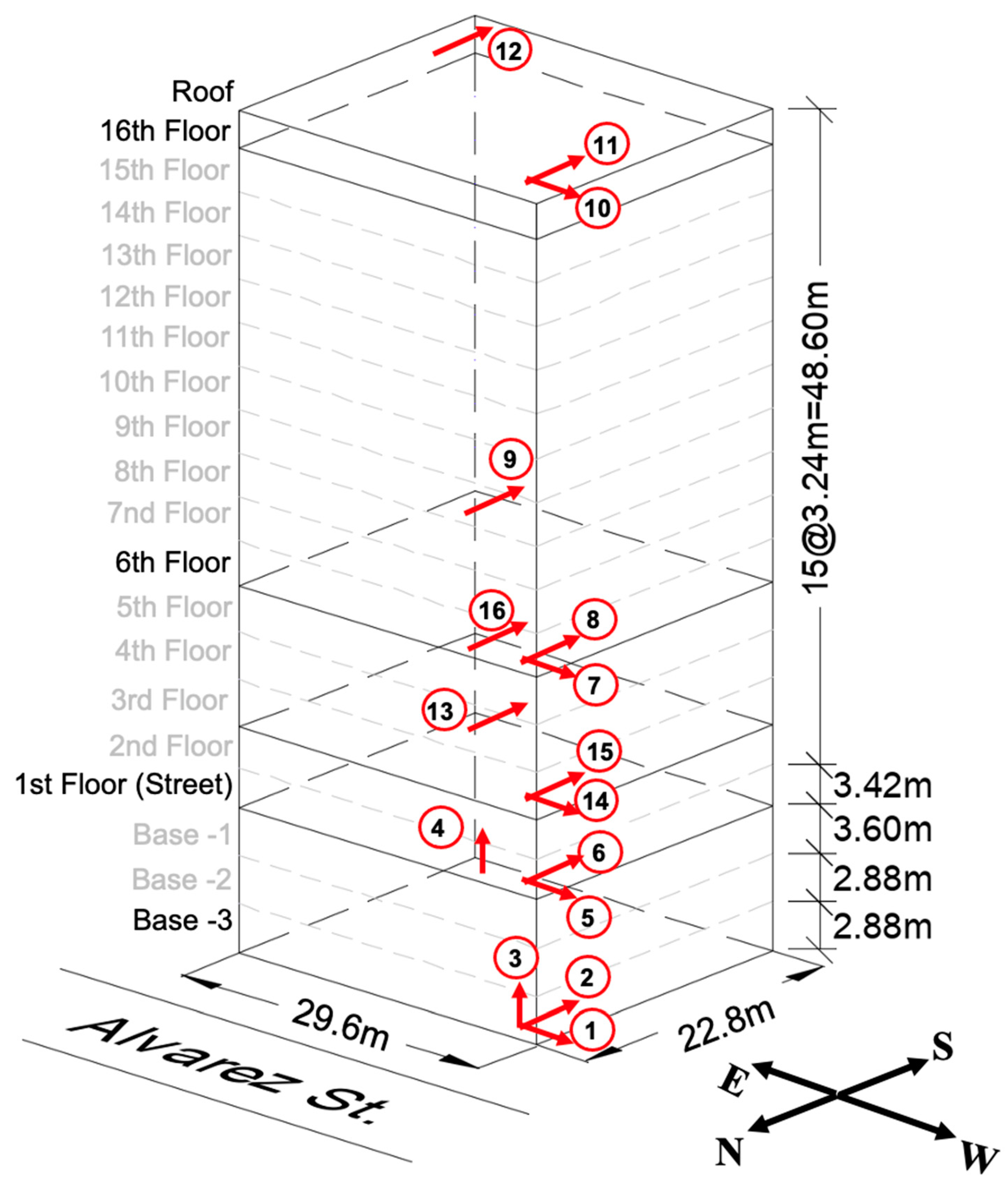
The case study corresponds to a sixteen-story building office with three additional basement stories, where the first story is 3.42 in height and stories 2–16 are 3.24 in height. It is situated in Viña del Mar, located in the Chilean central coast area, where several buildings were damaged during the last Mw 8.8 Maule earthquake. A picture of the building and a typical plan view are depicted in Figure 1. The structure was built in 2008, following the 2004 Chilean Building Code, which refers to the ACI–318 concrete design provision [27]. It is designed and built as an RC dual system (i.e., core structural wall and perimeter moment frame-wall), which is a typical construction type for offices in Chile. The monitoring time is between 27 March 2010 and 19 April 2011. During the monitoring period, the building was equipped with 16 force–balance Digitexx uniaxial accelerometers model D–110U (see

Table 2. Specifications of the Digitexx uniaxial accelerometers.

Specification	Parameter
Acceleration range	+/−3 (g)
Output	1.2 (V/g) standard between 2000 (Ω) or greater
Load capacitance	10.000 (pF) maximum
Transverse axis	0.005 (g/g)
Linear error	<±0.2% F.S.
Noise threshold	<1 (μg/√Hz) (Band 0.05–1.500 (Hz))
Dynamic interval	>110 (dB)
Bandwidth	DC–2.000 (Hz) to 3 (dB)
Power	+/−12 (Vdc), 9 (mA)
Operating temperature	−40 (°C) to +85 (°C)
Zero axis variation due to change	<200 (μg/°C) outside temperature range
Cover	Pressurized hermetic aluminum housing
Dimensions	108 × 76 × 57 (mm)
Mass	0.5 (kg)

for detailed specifications) distributed with the height and across the floor. Four (4) sensors were installed on the third underground level, three (3) on the ground surface level, and then three (3) sensors on the third, sixth, and top floor. It is worth mentioning that the two vertical sensors 3 and 4 in the 3rd subterranean floor were not activated. The sensors register accelerations along the two horizontal directions of the building, where one sensor measured in the EW direction and two sensors in the NS direction. The criteria followed for the chosen positions of the instruments was in such a way that torsional modes are identified, given that the distribution of walls and columns with non-coincidental mass and rigidity centers naturally is expected to cause torsional behavior. Additionally, this sensor distribution allowed for the monitoring of the structure’s spatial motion, the partial capturing of its linear and nonlinear response features since no sensors were available on the intermediate floors (from the 7th to the 16th), The sampling rate for the sensors was 100 Hz. Figure 2 shows a diagram illustrating the array of 16 accelerometers temporarily deployed in the building. General information corresponding to the mounting of the accelerometer array can be found elsewhere [28].

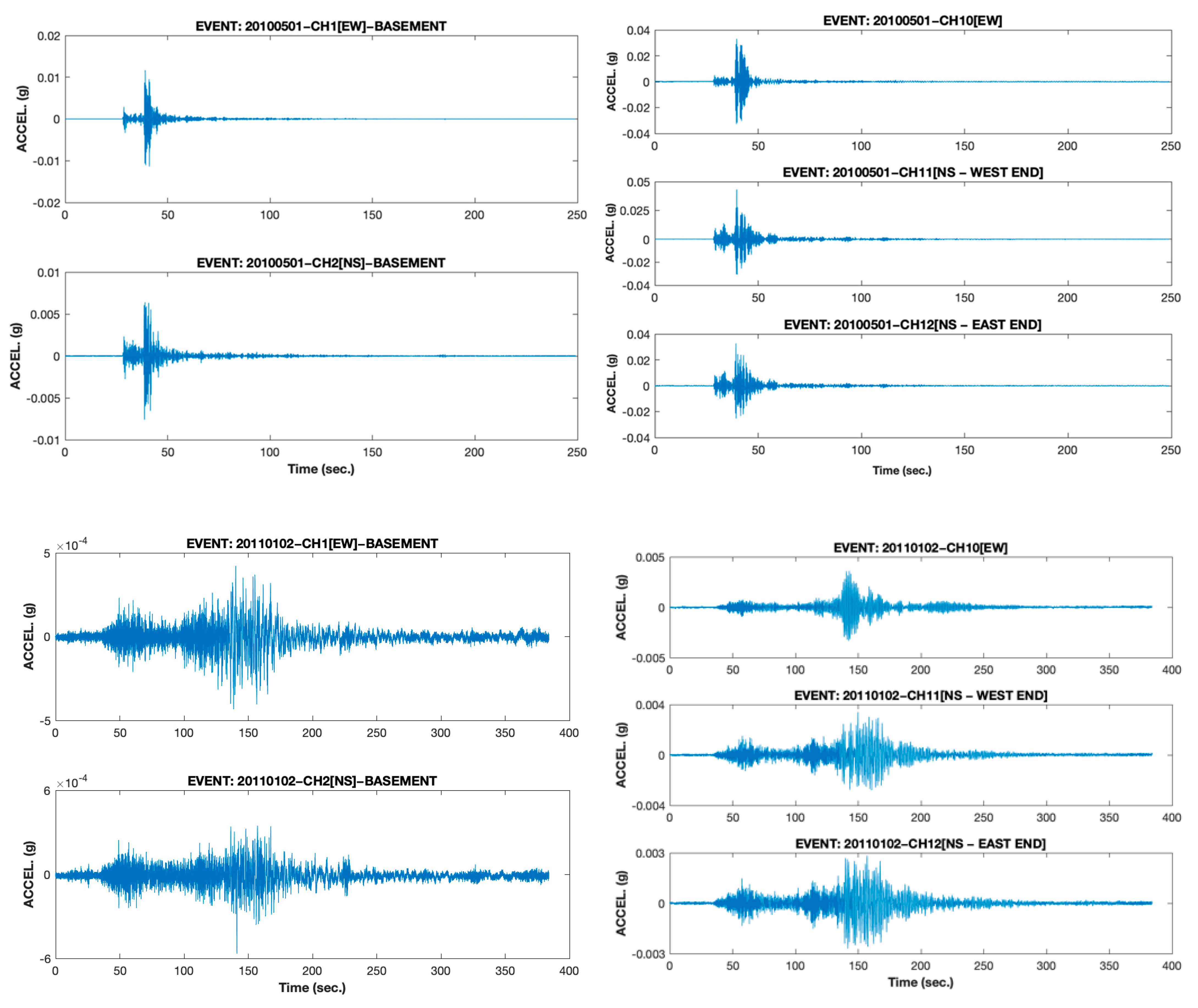
Figure 3 shows the acceleration time-histories of the response recorded by channels 1–2 at the basement and channels 10–12 at the ceiling of the 16th floor (roof level) of the building to the events that occurred on 1 May 2010 and 2 January 2011 (Table 1). The former Mw 5.0 event was located approximately 73 km south-west of Viña del Mar, and the latter Mw 7.2 event was located 42 km north-west of Carahue and approximately 611 km south of Viña del Mar. Response data from these and the other events listed in Table 1 will be used to perform detailed analyses.

2.2. Signal Processing

To perform the analysis correctly regardless of the method, it is important to verify that the input value is accurate. Many parameters can interfere in the data collection process, such as poorly installed instrumentation, as well as inconsistencies in the reception of data, for example, files that are in bad condition or confusion regarding the units of measurement. It must be made clear that these parameters depend entirely on the instrumentation. With technological advances, the instruments can correct all of these problems automatically, but taking these factors into account, in the case of this article, only one parameter is adjusted to be able to apply the two methods in question, namely the correction of the signal baseline.

Baseline Correction

This occurs when the registers, to perform the analysis, are displaced with respect to the origin. This is a common problem where, due to installation issues, the instruments are not perfectly level. This issue may also arise when the vertical component of an earthquake causes a rebound effect with the surface.

Before the data can be correctly analyzed, they must be prepared via a convenient standardization procedure called a baseline correction, by which the sample values are transformed into a new set of values that have a sample average equal to zero [29].

As previously mentioned, the different methodologies currently used for the identification of dynamic properties in structures are separated into parametric and nonparametric techniques. In the following sections, the procedures of both general methodologies are defined.

2.3. Parametric Analysis Procedure

In this procedure, a simplified mathematical model is used, and the values of the structural parameters necessary to produce an optimal correlation between the measured and calculated responses are estimated. For the latter, the theory of structural analysis and dynamics is used to model the structure and obtain its properties [21,26,30]. Within this category are methods such as the prediction error method (PEM) and stochastic subspace identification (SSI) technique for linear systems. Both are time-domain methods (i.e., they work directly with temporal data without the need to convert them into correlations or spectra) [31]. For this study, we employ the SSI technique, which was published by Peter Van Overschee and Bart De Moor in 1996 [32].

To perform system identification by means of the SSI method, it is necessary to understand how dynamical systems are represented in their state-space form and how it is possible to obtain relevant system information through this representation. First, the dynamic equation of the system must be stated in the traditional form according to the following equation:

$${\mathit{M}}_s\ddot{\mathit{x}}+{\mathit{C}}_s\dot{\mathit{x}}+{\mathit{K}}_s\mathit{x}=\Lambda u-{\mathit{M}}_s\Gamma {\ddot{\mathit{x}}}_g$$

(1)

where $\mathit{x}\in {ℝ}^{nx1}$ is the vector of displacements relative to the ground of the n floors or degrees of freedom of the structure; ${\ddot{\mathit{x}}}_g$ is the ground acceleration; $\Gamma$ is the seismic participation vector; and $\Lambda$ indicates the location of the control signal u if any. For the purposes of this study, $\mathit{u}=0$.

The advantage of the SSI technique is that it performs its analysis only with data that can be directly measured on the structure (only output data), such as the accelerations of the ℓ floors where the accelerometers are installed. In addition, the main assumption of this method is that the measurements obtained by the system correspond to natural stochastic vibrations caused by a white noise type of disturbance ${\mathit{w}}_k$ as well as electrical noise ${\mathit{v}}_k$ in the measuring devices; however, these types of noise are not related to each other. The development of this technique and its mathematical foundations are realized in the time domain by the state-space representation of the dynamical system under study defined as:

$${\mathit{z}}_{k+1}={\mathit{A}}_d{\mathit{z}}_k+{\mathit{w}}_k$$

(2)

$${\mathit{y}}_k={\mathit{C}}_d{\mathit{z}}_k+{\mathit{v}}_k$$

(3)

where $\mathit{y}$ is the measured structural response and $\mathit{z}$ is the vector of states. The subscript k of the time variables corresponds to the time instant ${\mathit{t}}_k=k·\mathsf{\Delta }\mathrm{t}$.

The main objectives of this method are to determine the order $n_s=2n$ of the system and to obtain the matrices ${\mathit{A}}_d$ and ${\mathit{C}}_d$.

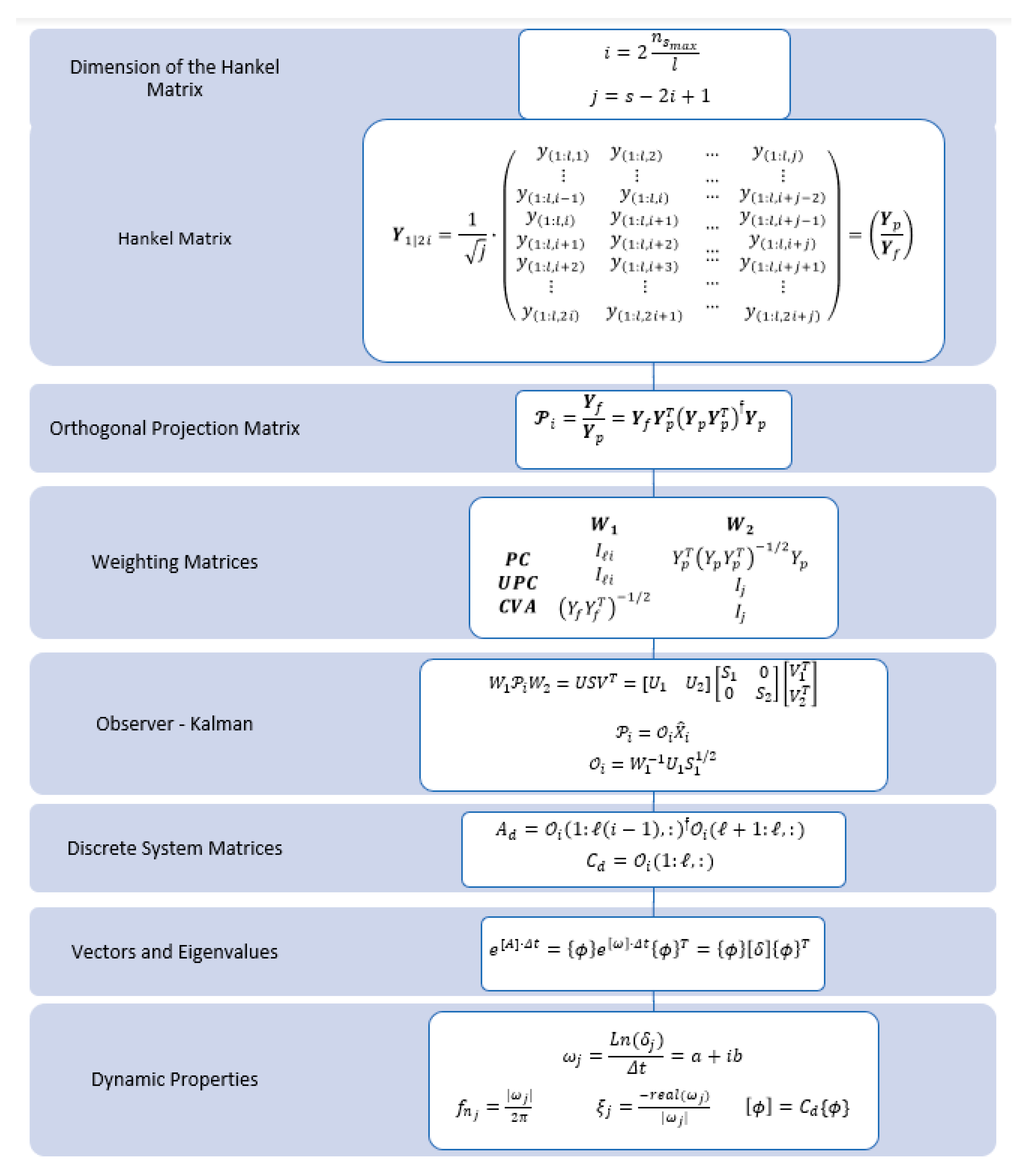
2.3.1. Hankel Matrix

The Hankel matrix constitutes the basis of all of the formulations that have been developed with the SSI technique. The matrix has dimensions of $2i\ell \mathrm{x} \mathrm{j}$, where ℓ is the number of sensors arranged in the structure, $i=2\frac{n_{s_{max}}}{\ell }$, $j=s-2i+1$, $s$ is the number of measurements performed on the structural system, and $n_{s\left(max\right)}$ corresponds to the maximum order of the system, which should be neither too small nor too large and is estimated by the engineer. The upper part of the matrix corresponds to the past, and the lower part corresponds to the future.

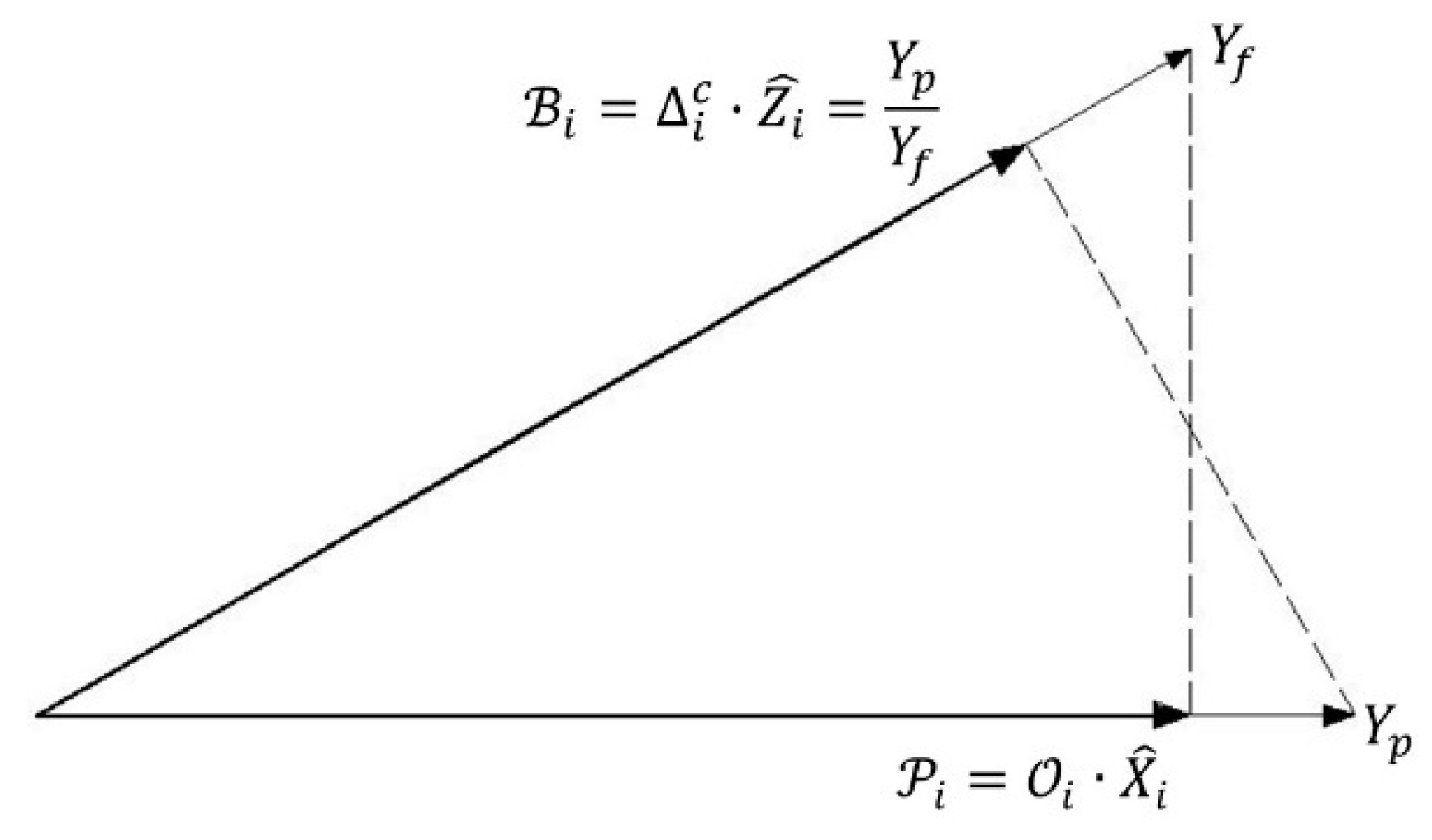
2.3.2. Projection of Blocks (${𝒫}_i$)

The projection ${𝒫}_i$ is defined by the orthogonal projection matrix of the SSI method and is determined as the product between the observability matrix ${\mathcal{O}}_i$ and the estimated sequence of states of the Kalman filter ${\widehat{\mathit{X}}}_i$. This procedure is depicted in Figure 4. The orthogonal projection of the future outputs ${\mathit{Y}}_f$ onto past outputs ${\mathit{Y}}_p$ determines the forward state sequence ${\widehat{\mathit{X}}}_i$. Conversely, the orthogonal projection of past outputs ${\mathit{Y}}_p$ onto the future outputs ${\mathit{Y}}_f$ determines the backward state sequence ${\widehat{\mathit{Z}}}_i$ [32]. Figure 4 also presents the variables ${\mathsf{∆}}_i^c$ and ${\mathit{ℬ}}_i$, which correspond to a controllability matrix and the projection of past outputs onto the future outputs, respectively However, these variables are not part of the procedure since they serve only to define and understand the origin of the projection of blocks ${\mathit{𝒫}}_i$.

2.3.3. Singular Value Matrix of the Orthogonal Projection Matrix $\left(\mathit{S}\right)$

The orthogonal projection matrix is decomposed into its singular values considering the pre- and post-multiplication of the so-called weighting matrices. The diagonal matrix $S$ is of order $m$, which indicates the order $n_s$ of the system with $m=n_s$. The criterion for defining the value of m depends on the assignment of the weighting matrices.

2.3.4. Weighting Matrices of the Orthogonal Projection Matrix (${\mathit{W}}_1$ and ${\mathit{W}}_2$)

There are three algorithms with which the weighting matrices can be defined:

• The principal component (PC) algorithm.
• The unweighted principal component (UPC) algorithm.
• The canonical variant algorithm (CVA).

The first two algorithms calculate the order $m$ of the singular value matrix by detecting the position at which the diagonal of the matrix $S$ starts to become zero. On the other hand, the CVA calculates the order m by detecting the position at which the values of the diagonal of the matrix $S$ stop converging to one, where the tolerance is defined by the engineer.

2.3.5. Eigenvalues ($\mathit{\delta }$) and Eigenvectors ($\mathit{\varphi })$

The eigenvalues and eigenvectors are calculated from the discrete system matrices ${\mathit{A}}_d$ and ${\mathit{C}}_d$. The vector $\mathit{\delta }$ is used to calculate the identified frequencies of the system, and $\mathit{\varphi }$ denotes the vibrational shapes corresponding to the abovementioned frequencies.

2.3.6. Damping Fraction ($\xi$)

Damping is a property of the system and includes a large number of phenomena that, if the system is left to vibrate freely after an initial excitation has been applied to it, will eventually dissipate [9].

Figure 5 shows a flow chart of the SSI method.

2.4. Nonparametric Method

Nonparametric methods are based on applying a set of mathematical procedures, transformations and functions to the signals obtained from the acceleration records. These accelerometer records correspond to variables that are functions of time. One of the main characteristics of nonparametric methods is to perform an analysis of the records as a function of frequency, thereby determining how the energy or power of the signal is distributed. 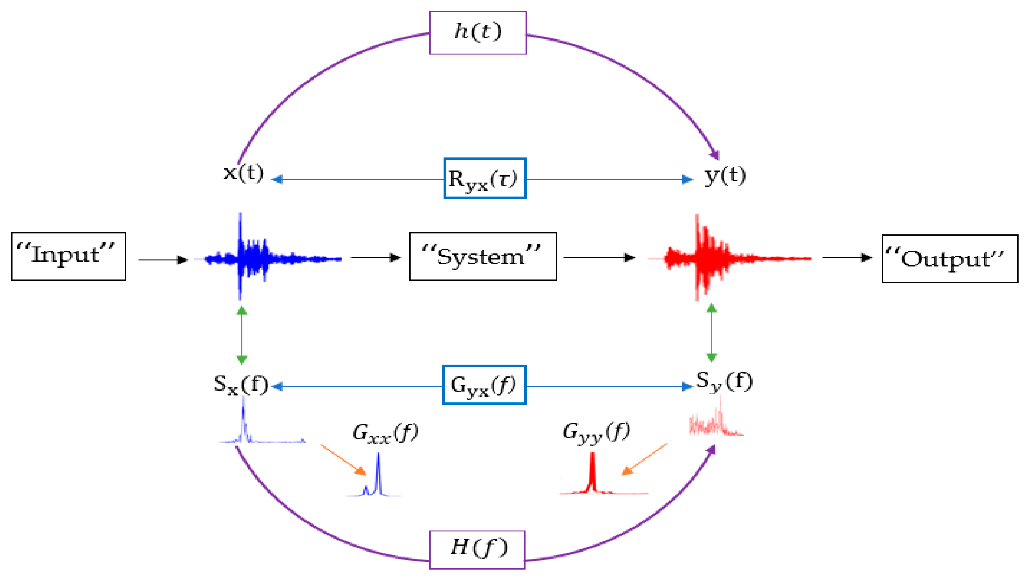The processes described in Figure 6 allow the specific properties of the system to be identified.

In the above figure, $x\left(t\right)$ is the time-domain input signal; $y\left(t\right)$ is the time-domain output signal; $h\left(t\right)$ is the impulsive system response; $S_x\left(f\right)$ is the linear Fourier spectrum of x(t); $S_y\left(f\right)$ is the linear Fourier spectrum of y(t); $H\left(f\right)$ is the system transfer function; $R_{yx}$(τ) is the cross-correlation of x(t) and y(t); $G_{xx}$(f) is the spectral power of x(t); $G_{yy}$(f) is the spectral power of y(t); and $G_{yx}$(f) is the cross-spectral power of x(t) and y(t).

To obtain the dynamic properties of the system, a series of procedures are followed based on the authors’ criteria. The process is briefly described in the following subsections.

2.4.1. Obtaining the Spectral Density

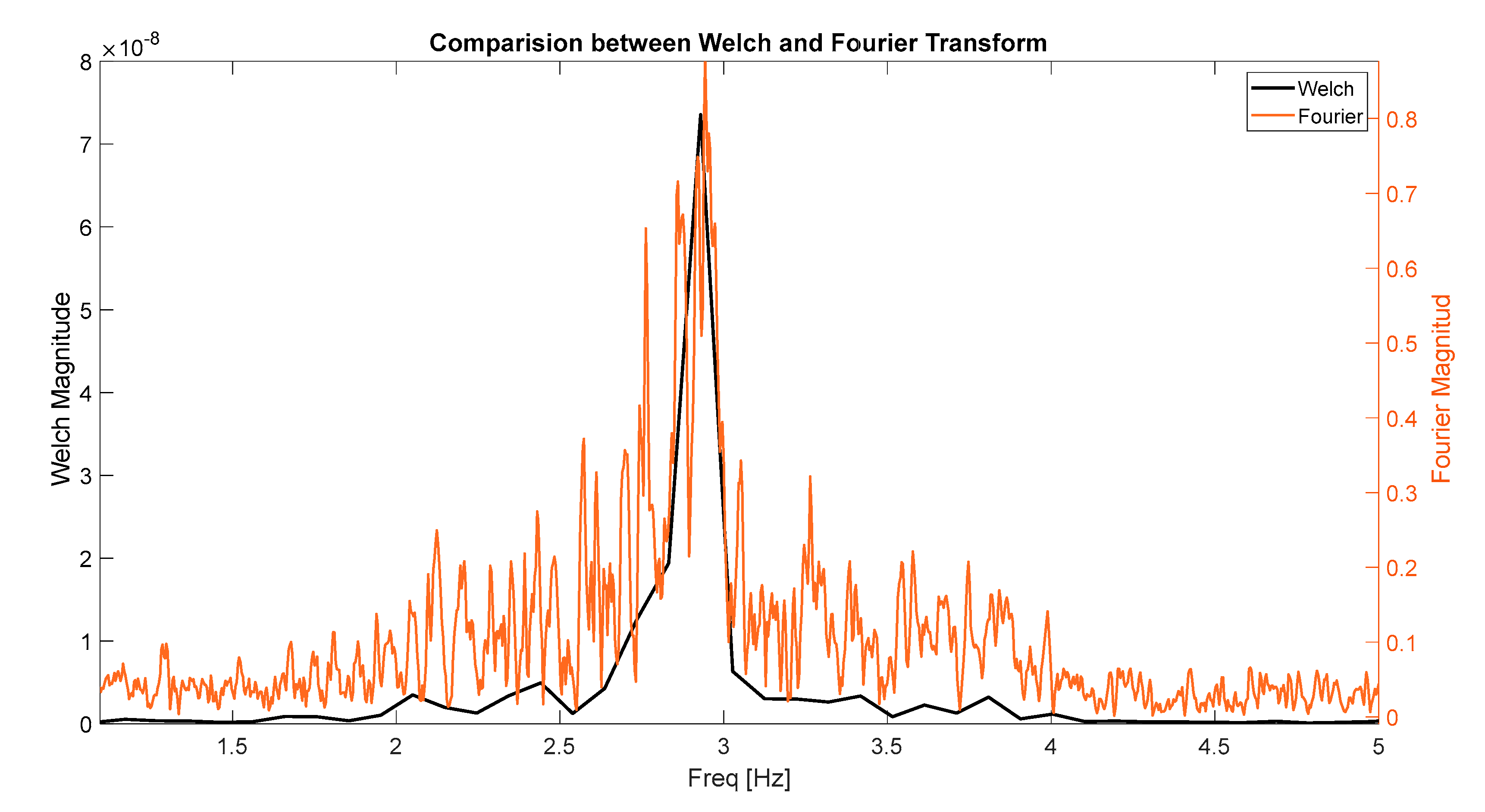
As previously mentioned, the Fourier transform identifies important frequencies from an engineering point of view and has become the dominant method [29]. Accordingly, new techniques have been created and improved based on the Fourier transform, as in the case chosen for this analysis, for which the Welch power spectral density estimation ($G_{xx}$) is used. The Welch power spectrum works with superimposed segments, increasing the frequency resolution and allowing the spectrum to be observed better. Figure 7 shows a spectrum obtained using the Fourier transform superposed onto the Welch spectrum.

2.4.2. Correlations

Correlation functions can acquire parameters to quantify how similar these signals are; these functions include autocorrelation, which analyzes how much a signal varies over time, and cross-correlation, which measures the similarity of two signals. The theoretical processes are as follows:

$$R_{xx}\left(\tau \right)=\underset{T\to \infty }{\lim }\frac{1}{T}{{\displaystyle \int }}_0^{T}x\left(t\right) x\left(t+\tau \right)dt$$

(4)

$$R_{xy}\left(\tau \right)=\underset{T\to \infty }{\lim }\frac{1}{T}{{\displaystyle \int }}_0^{T}x\left(t\right) y\left(t+\tau \right)dt$$

(5)

These can also be estimated by using power spectral density functions ($G_{xx}$ and $G_{yx})$.

2.4.3. Phase

It must be taken into consideration that the functions with which the nonparametric method works are sometimes complex variables. Examples include the Fourier transform and cross-power correlations. Complex variables play an important role in calculating vibration shapes since they reveal whether the relative motion between two points occurs in the same direction.

The numerical value given by the phase angle varies only within $\pm \pi$. Thus, a phase angle equal to 0 between 2 different points at an analyzed frequency indicates that the direction of motion is the same, called being in phase. Otherwise, if the phase angle is $\pm \pi$, the relative movement is opposing, known as a phase shift. The formulae used to obtain the phase angle of a complex variable are as follows:

$$G_{xy}\left(f\right)=A_{xy}\left(f\right)+i{B}_{xy}\left(f\right)$$

(6)

$$\left|Gxy \left(f\right)\right|=\sqrt{A_{xy}{}^2\left(f\right)+i{B}_{xy}{}^2\left(f\right)}$$

(7)

$${\theta }_{xy}\left(f\right)={\tan }^{-1}\frac{B_{xy}\left(f\right)}{A_{xy}\left(f\right)}$$

(8)

2.4.4. Transfer Functions

Transfer function describe the dynamic characteristics of a linear system. These functions can be calculated directly through Fourier spectral densities, but a risk arises for certain frequencies where the mathematical procedure is affected. Instead, the power spectra are used to determine the transfer functions, but this approach is applicable only for random vibrations, and the consistency must be measured by means of the coherence function.

$$H\left(f\right)=\frac{S_y\left(f\right)}{S_x\left(f\right)}$$

(9)

$$H1\left(f\right)=\frac{G_{xy}\left(\mathrm{f}\right)}{G_{xx}\left(\mathrm{f}\right)}$$

(10)

$$H2\left(f\right)=\frac{G_{yy}\left(\mathrm{f}\right)}{G_{yx}\left(\mathrm{f}\right)}$$

(11)

2.4.5. Coherence Function

This concept is crucial for differences in frequencies that are particularly important in the analysis. Theoretically, this function provides a good estimate of the energy output due exclusively to the input signal. The coherence function is a dimensionless frequency function that has only the real part and delivers values in the range from 0 to 1. For analysis, this function reflects how consistent the output signal is with the input signal. For example, in a comparison between the records of the second floor and the last floor, the coherence function can be used to determine how consistent the records are and can differentiate a certain frequency of the structure for one of the floors.

$${\gamma }^2{}_{xy}\left(f\right)=\frac{H_1\left(f\right)}{H_2\left(f\right)}=\frac{{\left|G_{xy}\left(f\right)\right|}^2}{G_{xx}\left(f\right)G_{yy}\left(f\right)}$$

(12)

2.5. Analysis Procedure of the Nonparametric Method

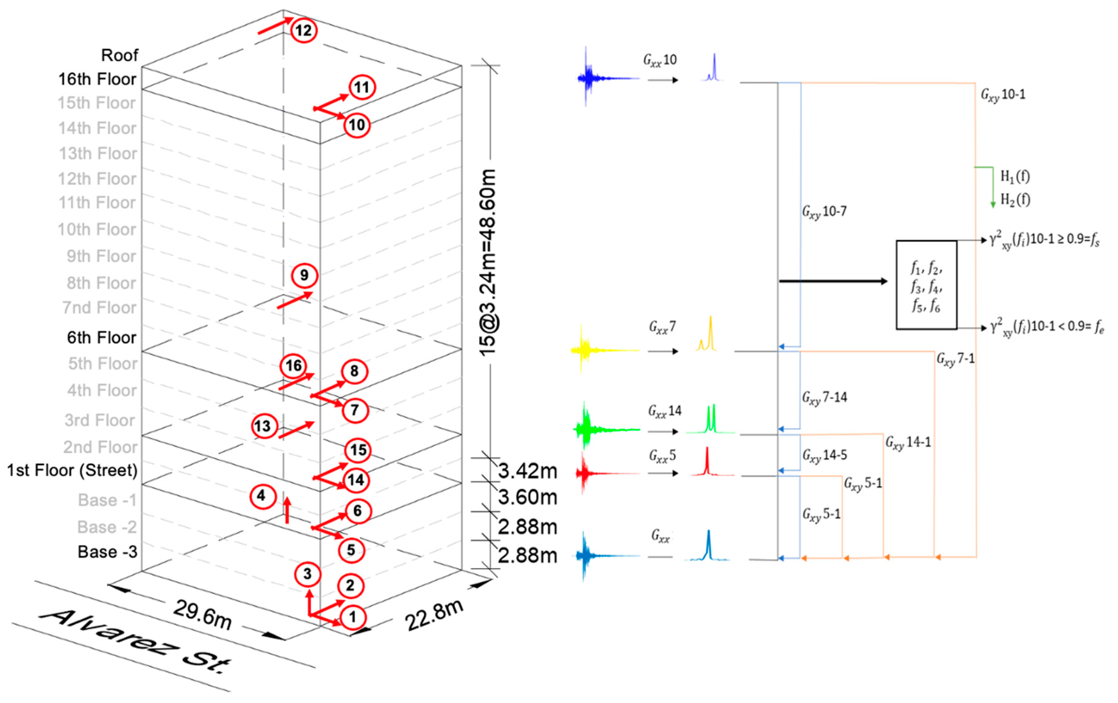
Considering the concepts explained above, this subsection details the use of the nonparametric approach and the criteria applied to obtain the dynamic parameters. To better understand the problem under study, a diagram with sensors ordered by floor is presented in Figure 8.

With the acceleration records sorted by floor, we proceed to obtain the Welch power spectra ($G_{xx}$). The first criterion is that only the first six frequencies (i.e., the six frequencies with the highest amplitudes) are identified due to the fact that for structural dynamic analysis, we are interested only in a certain range of frequencies for analysis. Outside that range, for this study case, the frequencies have no physical importance.

The next step is to analyze whether the identified frequencies correspond to the frequencies of the floor or of the structure. To this end, the cross-power correlation between the signal of the first floor and that of the last floor ($G_{xy}$) is calculated. With the obtained correlation and the Welch power spectrum, it is possible to obtain the transfer functions $H_1\left(f\right)$ and $H_2\left(f\right)$, and with these values, the coherence function between floor −3 and floor 16 can be acquired. Here, a second criterion is applied to the analysis of the result of the coherence function (${\gamma }^2{}_{xy}$). If the value of this variable is greater than 0.9, frequency corresponds to the soil ($f_s$). This is due to the fact that having a coherence greater than 0.9 means that the movement of the last floor is mostly a product of the movement of floor −3, i.e., the floor in direct contact with the ground. Nevertheless, an analysis of the soil frequencies is beyond the scope of this article.

Once the frequencies of the structure have been identified, only whether they correspond to translational or torsional frequencies remains to be checked. For this purpose, the registers on opposite corners of the same floor are correlated. The phase angle between these signals on the same floor is verified, and the last criterion is used, to verify whether the result of the phase angle is less than 1. If so, the relative movement is in the same direction, which is interpreted as a translational movement.

With the translational frequencies of the structure, we proceed to identify the modal shapes by performing three types of correlations. The first is to correlate all floors with the −3 and obtain the relative displacements with the phase angles. The second option is to take continuous correlations between floors and likewise obtain relative displacements with the phase angles. A third correlation is performed. This is created after appreciating the results between the parametric and non-parametric method in which a way to improve the results is sought, where it is correlated up to floor 3 with -3 and then correlated floor with floor up to 16.

Finally, following these three calculations, the amplitudes of the modes can be obtained through the Welch power spectrum, and the vibration shapes can be normalized. These three ways of correlating the signals are discussed in detail in the results.

3. Results

This section presents the results by date for both methods, including the mode shapes with their normalized amplitudes and their respective relative directions (Figure 9).

Table 3. Identified torsional frequencies of the building for the selected events.

Date	Torsional Frequency [Hz]
5 April 2010	3.32	4.00
1 May 2010	3.91	5.08
23 October 2010	5.27	-
2 January 2011	0.88	-
21 January 2011	3.22	-
14 February 2011	1.07	3.52

presents the torsional frequencies of the building obtained from each method for the selected seismic events. It is worth noting that the building was in the rough-in stage over this period. The damping value obtained from each method is also presented in Table 3 and

Table 4. Damping for the parametric method algorithms according to date, direction of analysis, and identified translational frequency.

Date	Direction	Frequency [Hz]	$\mathit{\xi }$ PC [%]	$\mathit{\xi }$ CVA [%]	$\mathit{\xi }$ UPC [%]
5 April 2010	EW	6.64	0.51	5.09	1.4
	NS	2.44	1.77	1.91	1.29
1 May 2010	EW	3.22	0.7	2.24	1.65
	EW	3.91	1.25	−0.55	0.64
	NS	2.44	1.65	10.01	1.25
23 October 2010	EW	6.74	1.7	−0.04	0.35
	NS	0.68	0.78	1.33	0.84
	NS	3.42	1.85	2.36	0.91
2 January 2011	EW	2.64	2.37	2.85	1.45
	EW	3.42	1.8	2.98	4
	NS	0.68	2.61	1.8	2.1
	NS	2.63	2.35	3.24	2.35
21 January 2011	EW	0.88	0.34	0.21	0.42
	EW	6.84	1.11	0.73	0.64
	NS	2.64	2	0.96	1.61
14 February 2011	EW	2.64	2.02	1.12	1.48
	EW	3.14	14.67	1.65	0.23

. For the parametric case, the three defined algorithms (PC, CVA, and UPC) are presented, while for the nonparametric case, the results are presented using the 3 types of correlations, namely, the Bendat and Piersol floor-floor and Bendat and Piersol base-floor correlations, Bendat and Piersol EIC.

4. Discussion

4.1. Identified Frequencies

From a total of 11 records of seismic events, 12 frequencies are identified for the east-west direction, and 8 frequencies are identified for the north-south direction.

Table 5. Identified frequencies in the east-west direction for the parametric and nonparametric methods.

Frequencies [Hz]
Date	CVA	PC	UPC	Bendat and Piersol
5 April 2010	6.59	6.55	6.57	6.64
1 May 2010	3.15–3.88	3.21–3.87	3.22–3.94	3.22–3.90
23 October 2010	0.84–1.14–6.60	0.85–1.14–6.75	0.86–1.10–6.72	0.88–1.07–6.74
2 January 2011	2.68–3.33	2.62–3.36	2.61–3.41	2.63–3.42
21 January 2011	0.86–6.86	0.86–6.86	0.85–6.84	0.88–6.84
14 February 2011	2.60–3.13	2.64–3.20	2.61–3.24	2.64–3.14

and

Table 6. Identified frequencies in the north-south direction for the parametric and nonparametric methods.

Frequencies [Hz]
Date	CVA	PC	UPC	Bendat and Piersol
5 April 2010	2.42	2.41	2.45	2.44
1 May 2010	2.51	2.51	2.37	2.44
23 October 2010	0.69–3.37	0.70–3.44	0.70–3.41	0.68–3.42
2 January 2011	0.69–2.61	0.69–2.64	0.69–2.64	0.68–2.63
21 January 2011	2.62	2.63	2.62	2.63
14 February 2011	-	-	-	0.69

show the performance of the methods in terms of the number of frequencies identified per direction.

In the east-west direction for all dates, both the parametric and the nonparametric method algorithms succeed in identifying the frequencies. Moreover, the frequencies identified for each seismic event are similar between the two methods. For the north-south direction on 14 February 2011, the algorithms of the parametric method are not able to identify the frequencies, but the identified frequencies on the previous dates are similar. This allows us to assume that the programs achieve similar results.

Similar frequencies are repeated on different dates. We assume that these represent the frequencies of the fundamental modes of vibration of the structure. A good way to compare these results would be to obtain the design frequencies of the structure. Figure 10 depicts the frequencies with the corresponding dates and their direction.

We note an interesting trend concerning the identified frequencies—the mass and stiffness of the building change during the construction period. On the one hand, for some lower frequencies, a decrease in the structure’s stiffness may be related not only to the change in mass but also as a result of crack development in concrete (including those at the micro-level) due to the previous earthquakes, an increase in the service load and long-term deflections, redistribution of internal forces, and sometimes as a result of moisture shrinkage and thermal strains fluctuations. The structuring is also important since it affects the building’s mass distribution and the implementation of non-structural elements, which also contribute to the stiffness differential. Therefore, it can be seen that the higher frequencies in time for both directions increase. On the other hand, the intermediate or low frequencies in the EW direction tend to decrease as time passes. The fact that they increase or decrease may be associated with one of the above factors contributing to the mode of vibrations.

Considering that the design frequencies of the first 6 modes are 0.497, 0.65, 0.88, 2.13, 3.23, and 3.70 Hz [28], it is possible to appreciate that the identified frequencies, in both the east-west and the north-south directions, are similar except for 0.497 Hz.

4.2. Vibration Modes

4.2.1. Parametric Method

For most of the records, the three algorithms have the same relative movement directions. However, the SSI method is not able to distinguish whether the identified frequency or period originates from the ground or from the structure or whether it is torsional or translational. In addition, the number of frequencies it identifies depends entirely on the order of the system assigned to it. Consequently, in this study, the nonparametric method is used to distinguish the translational frequencies of the structure, after which those frequencies are searched for in the SSI algorithm. In most cases, it is sufficient to assign a maximum system order equal to 200. However, for the frequencies on 23 October 2010, and 14 February 2011, system orders equal to 500 and 350, respectively, are used to ensure that the parametric frequencies are as similar as possible to the nonparametric frequencies.

4.2.2. Nonparametric Method

To obtain the relative displacements of the floors, various correlations can be performed. The configurations of the accelerometers from floor −3 to floor 6 are emplaced every 3 floors, while those on floors 16 and 6 are separated by 10 floors. The graphs of the vibration shapes plotted in the previous section illustrate how the structure vibrates according to the correlation of each record of the structure with the record located at the base, represented by floor −3 (the base-floor correlation). On the other hand, we can also observe how the building vibrates according to the correlation of each floor of the structure with the floor that precedes it (the floor-floor correlation). In this study, seeing how these graphs behave for all dates reveals that the best result is obtained by combining the correlations of floors 1 and 3 with the base and the correlations of floors 6 and 16 with the records that precede them. In this way, a third form of vibration is plotted, called the Bendat and Piersol EIC.

4.2.3. Comparison of Methods

The trends of the vibration shapes for both methods on most dates are congruent. That is, the amplitudes present the same relative displacements. In the previous sections, the results in terms of frequency show good agreement, suggesting that both methods manage to identify similar frequencies. Note that for the frequencies of 6.74 and 6.84 Hz on 23 October 2010, and 21 January 2011, respectively, the relative displacements of the 16th floor do not coincide with those from the SSI algorithm. However, in both cases, the CVA corresponds very well with the nonparametric algorithm. This is due to the fact that the frequencies are very high (or the periods are very small).

4.2.4. Damping

The damping values are highly dispersed for all of the dates analyzed. This parameter is, in principle, difficult to obtain. In the design stage, the response spectra of structures are obtained by assuming 5% damping. In this case, the techniques used work directly with the acceleration records of an earthquake, where sudden changes in the magnitudes can be marked in an instant, implying that the methods used to calculate the damping factor are not sufficiently reliable.

5. Conclusions

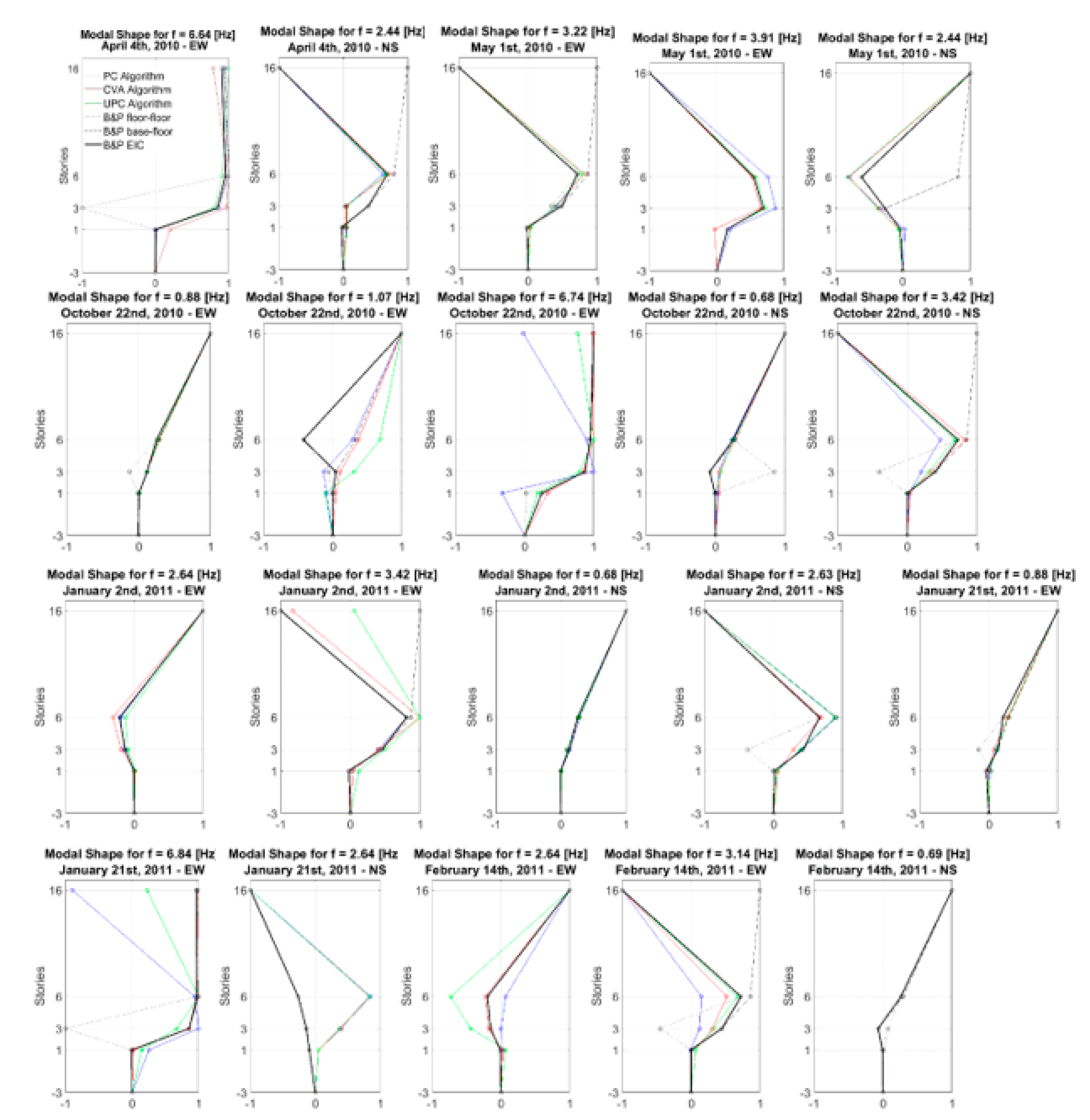
With the objective of comparing the parametric SSI method with the spectral nonparametric method by means of independent programs, six records of seismic events are analyzed, both methodologies are applied, and compatible results are obtained regarding the identified frequencies and forms of vibration.

Comparing the parametric and nonparametric methods reveals that the SSI method is less effective than the Welch spectrum identification method in the sense that the former is not able to distinguish whether the identified frequencies are rotational or translational and whether they correspond to the structure or the soil. In addition, the identification of frequencies in the SSI algorithm depends on the engineer’s criteria to assign an order to the system, which makes this approach unstable since the number of identified frequencies increases as the order of the system increases, whereas most of these frequencies are not recognized by the Welch spectrum.

The models created to determine the dynamic properties of the structure converge to similar results. However, this does not allow us to conclude that they closely approximate the reality. Implicitly, this marks a limitation that, in principle, can be improved. For this case, the seismic records are obtained from institutions, and there are detailed variables (specifically, in the signal processing subsection) for which it is not known whether they are within acceptable ranges. This limitation can be improved for future projects, where the monitoring campaign can be performed by the company itself, although it would require the acquisition of instruments. In this way, it would be possible to have better control of the variables that affect the calculation models, and the methods could be calibrated for future applications.

The application of these two methods allows for a range of results to be obtained, whereas in the case of this project, only the frequencies of structural interest are analyzed. Nevertheless, the fact that seismic-resistant structures are directly coupled to the soil, which transfers seismic excitations, should not be ignored. This article briefly mentions the difference between a soil frequency and a structural frequency and that, by means of the methods used, it is possible to separate and work only with the frequencies of the structure. Future research should analyze these frequencies, perhaps in an approach applied to soil-structure interactions.

Ultimately, the engineering importance of identifying the dynamic properties of structures lies in its potential for structural health monitoring, which is required for the modification of existing structures, structures subject to long-term movement or material degradation, fatigue assessment, and the development of a performance-based design philosophy [33,34,35].