
Reliability Analysis of Response-Controlled Buildings Using Fragility Curves


Abstract
:1. Introduction
2. IDA Pre-Requirements (Target Building, Dampers, and Input Earthquakes)
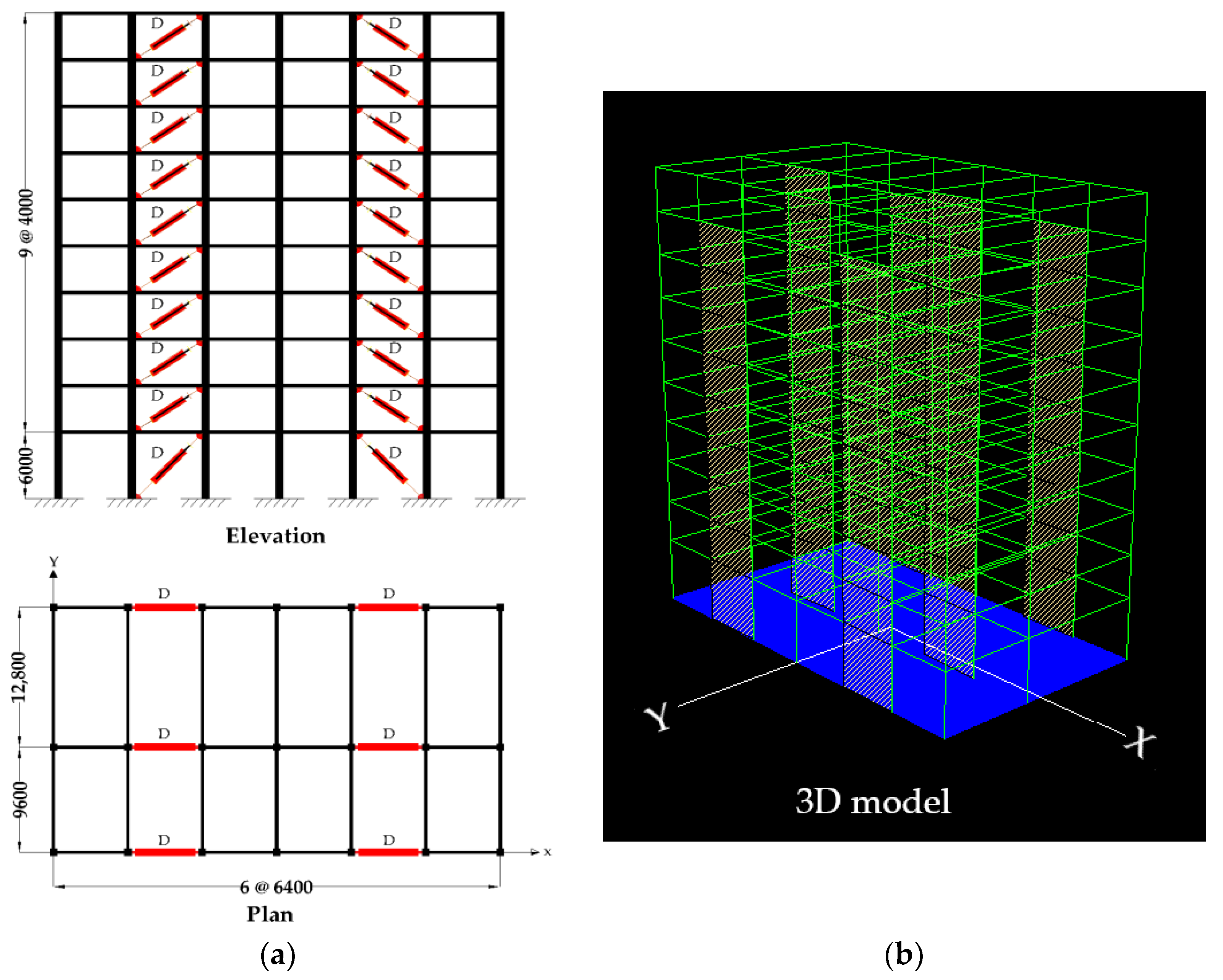
2.1. Target Buildings Description and Configurations
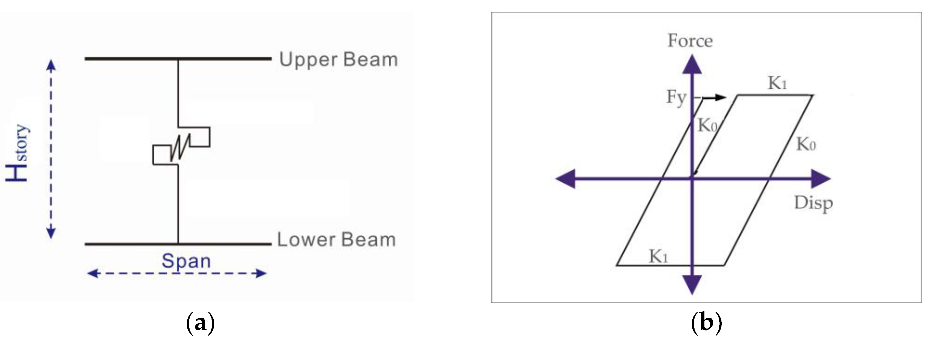
2.2. Passive Dampers
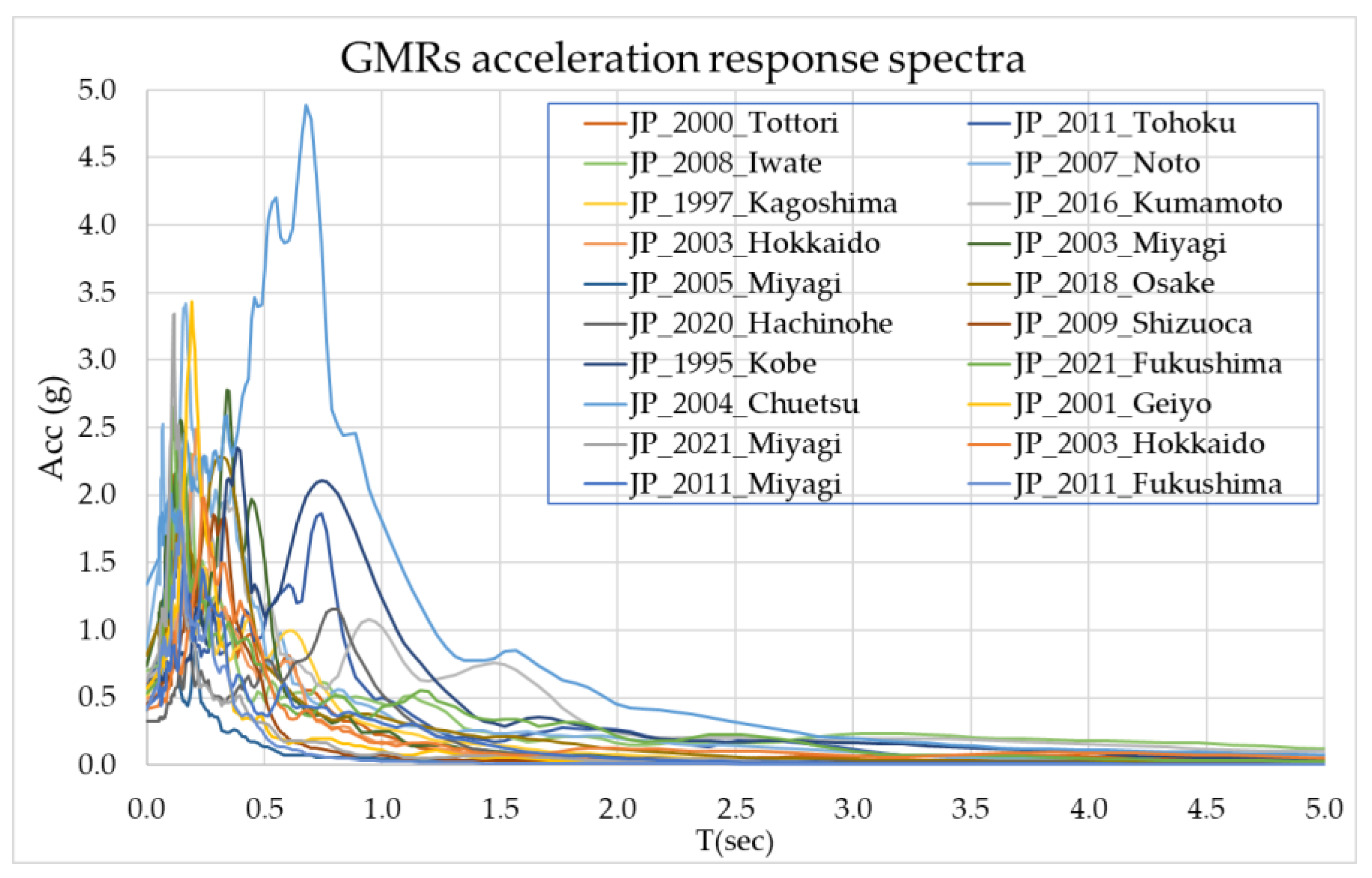
2.3. Ground Motion Record (GMR) Selection
3. Fragility Curve Based on Incremental Dynamic Analysis
3.1. Intensity Measure (IM) and Damage Measure (DM) Selection
3.2. Scale Factors
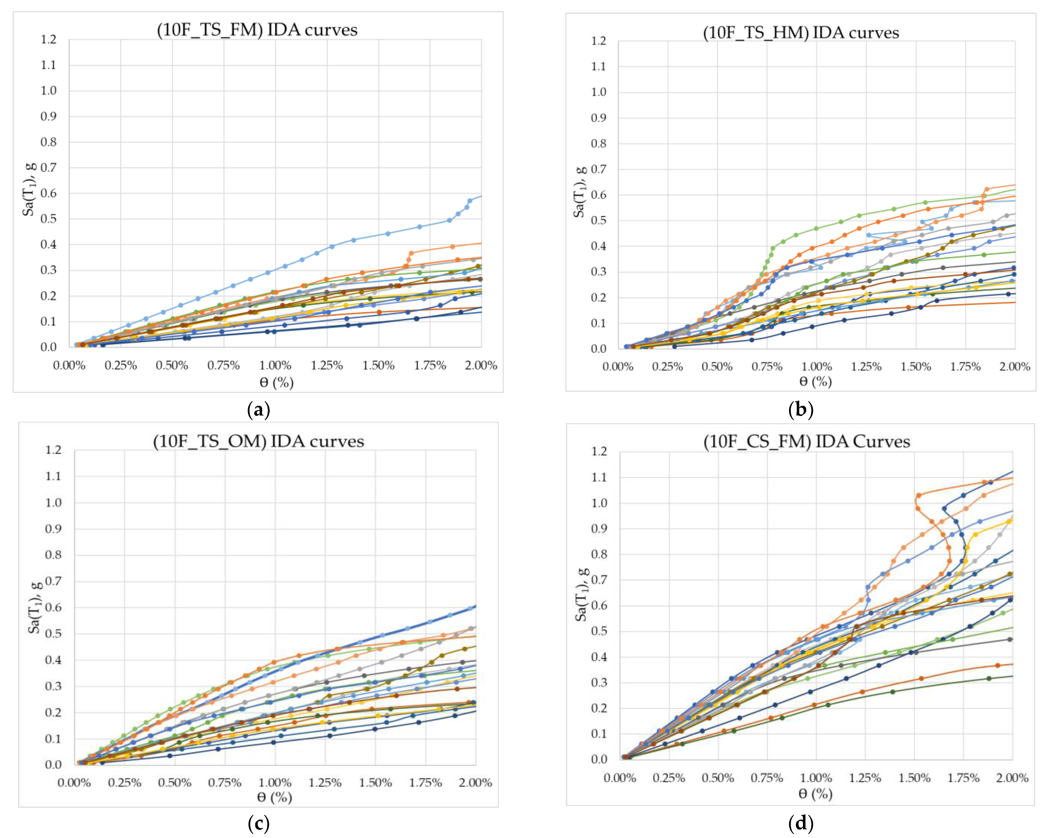
3.3. Applying IDA
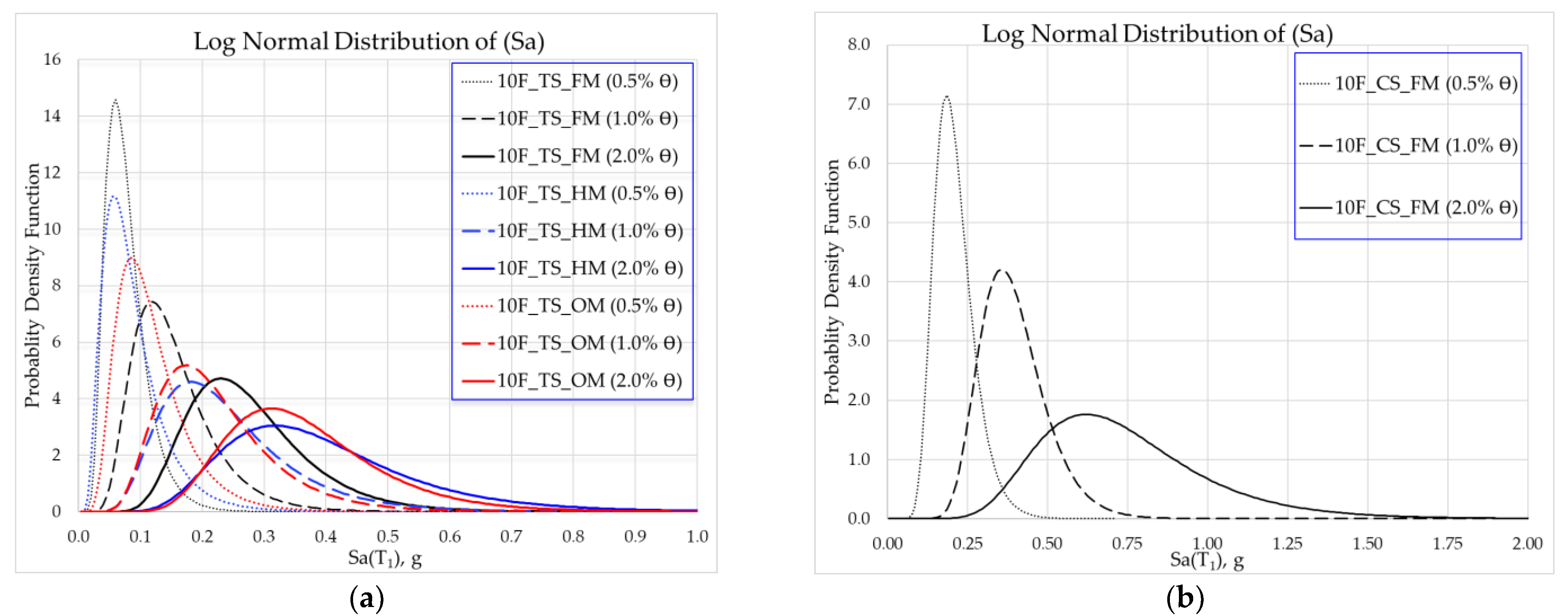
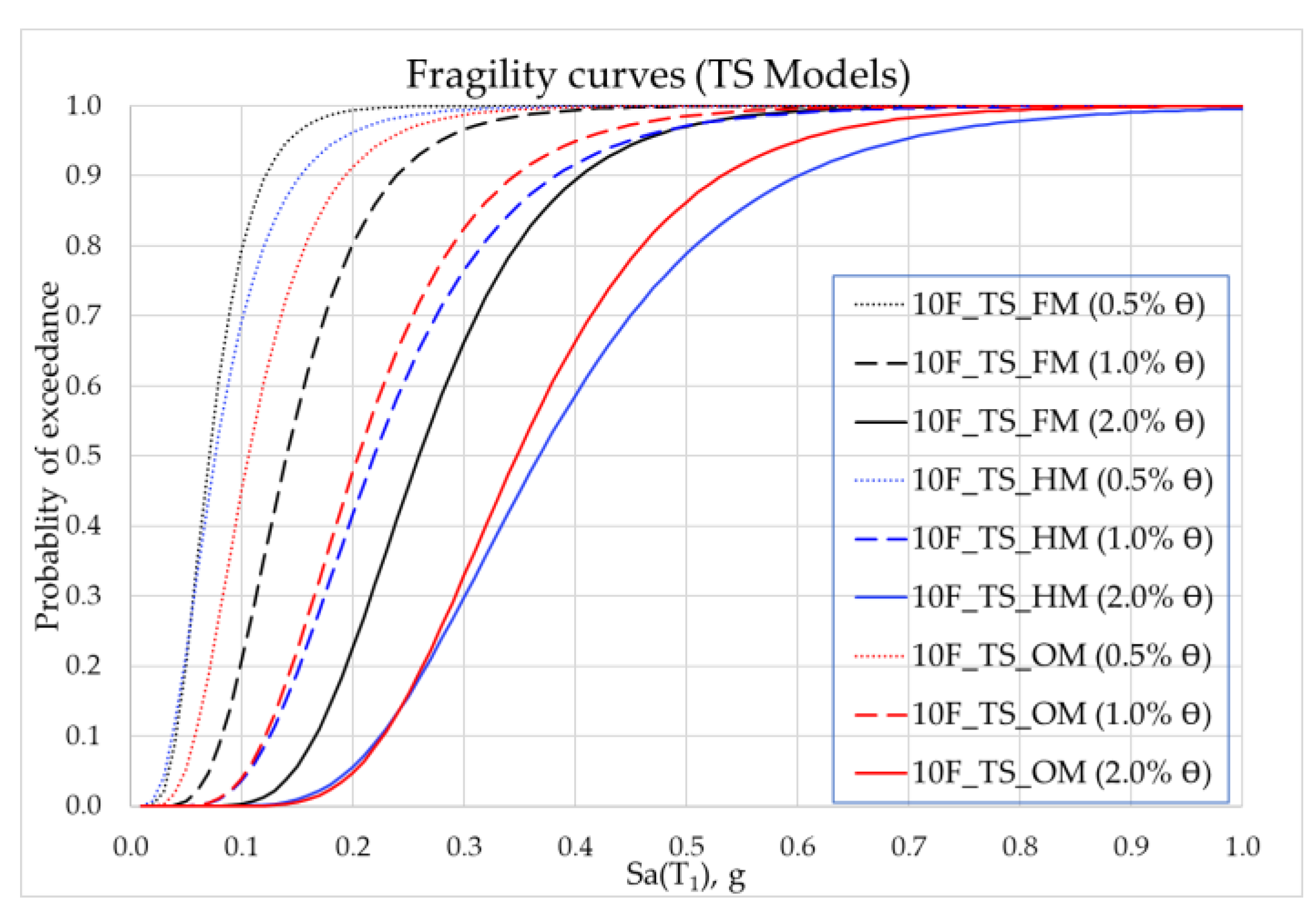
3.4. Fragility Curves
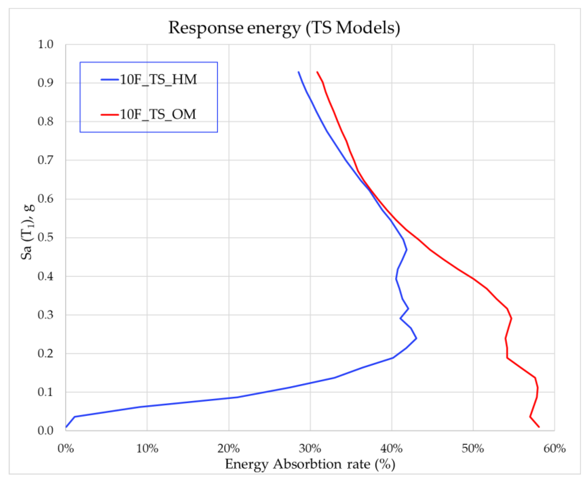
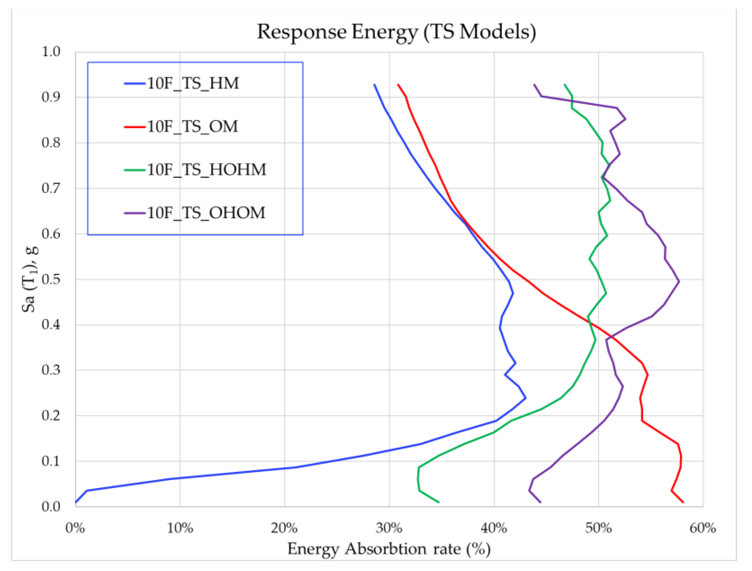
3.5. Response Energy of the Dampers
4. Combination of Different Types of Dampers
4.1. Combination of Hysteresis and Oil Dampers
4.2. Performance Evaluation of Combined Dampers Models
5. Conclusions
- The IDA is an effective method that can accurately predict the fragility assessment and reliability of response-controlled buildings.
- Sa(T1) is an efficient IM, since it has a good correlation with the seismic damage measures of first-mode-dominated structures. On the other hand, the story drift ratio θmax appeared to be an effective DM index. The lognormal cumulative distribution function provides a good understanding of damage probability with respect to the intensity of an earthquake at the certain damage level.
- Hysteresis and oil dampers effectively improved the seismic performance of the TS building.
- On the basis of the fragility curves, hysteresis dampers are more effective for larger ground motion accelerations than oil dampers.
- Oil dampers dissipated energy before hysteresis dampers for small deformations.
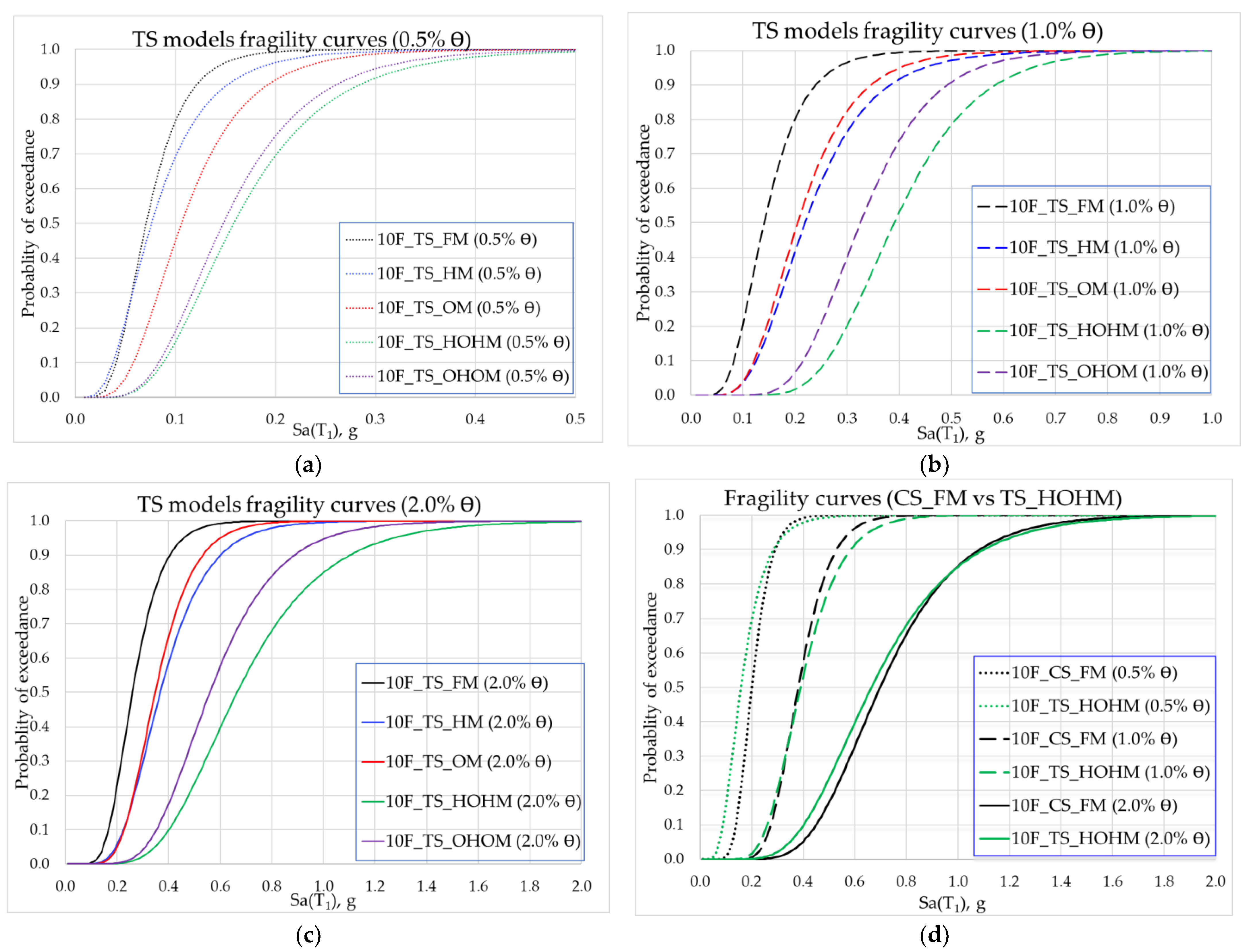
- Combined hysteresis and oil dampers in the TS buildings exhibited better performance than the individual hysteresis and oil damper buildings.
- The TS building equipped with a Hysteresis–Oil–Hysteresis damper configuration has almost the same performance as the CS building.
Author Contributions
Funding
Informed Consent Statement
Data Availability Statement
Conflicts of Interest
References
- Ikeda, Y.; Yamamoto, M.; Furuhashi, T.; Kurino, H. Recent research and development of structural control in Japan. Jpn. Archit. Rev. 2019, 2, 219–225. [Google Scholar] [CrossRef]
- Marko, J.; Thambiratnam, D.; Perera, N. Influence of damping systems on building structures subject to seismic effects. Eng. Struct. 2004, 26, 1939–1956. [Google Scholar] [CrossRef]
- Kasai, K.; Kibayashi, M. JSSI manual for building passive control technology part 1. In Proceedings of the 13th World Conference on Earthquake Engineering Vancouver, Vancouver, BC, Canada, 1–6 August 2004; p. 2989. [Google Scholar]
- JSSI. Manual for Design and Construction of Passively-Controlled Buildings, 3rd ed.; Japan Society of Seismic Isolation: Tokyo, Japan, 2013. (In Japanese) [Google Scholar]
- Kubilay, K. Seismic Base Isolation And Energy Absorbing Devices. Eur. Sci. J. ESJ 2013, 42–48. [Google Scholar] [CrossRef]
- Kam, W.Y.; Pampanin, S.; Palermo, A.; Carr, A.J. Self-centering structural systems with combination of hysteretic and viscous energy dissipations. Earthq. Eng. Struct. Dyn. 2010, 39, 1083–1108. [Google Scholar] [CrossRef]
- Chukka, N.D.K.R.; Krishnamurthy, M. Comparison of X-shaped metallic dampers with fluid viscous dampers and influence of their placement on seismic response of the building. Asian J. Civ. Eng. 2019, 20, 869–882. [Google Scholar] [CrossRef]
- Nicolas Luco, C.A.C. Structure-Specific Scalar Intensity Measures for Near-Source and Ordinary Earthquake Ground Motions. Earthq. Spectra 2007, 23, 357–392. [Google Scholar] [CrossRef] [Green Version]
- Del Gaudio, C.; Ricci, P.; Verderame, G.M.; Manfredi, G. Urban-scale seismic fragility assessment of RC buildings subjected to L’Aquila earthquake. Soil Dyn. Earthq. Eng. 2017, 96, 49–63. [Google Scholar] [CrossRef]
- Jalayer, F.; Cornell, C.A. Alternative non-linear demand estimation methods for probability-based seismic assessments. Earthq. Eng. Struct. Dyn. 2009, 38, 951–972. [Google Scholar] [CrossRef]
- Miano, A.; Jalayer, F.; Ebrahimian, H.; Prota, A. Cloud to IDA: Efficient fragility assessment with limited scaling. Earthq. Eng. Struct. Dyn. 2018, 47, 1124–1147. [Google Scholar] [CrossRef]
- Vamvatsikos, D.A.C. Incremental dynamic analysis. Earthq. Eng. Struct. Dyn. 2002, 31, 491–514. [Google Scholar] [CrossRef]
- Vamvatsikos, D.; Cornell, C.A. The incremental dynamic analysis and its application to performance-based earthquake engineering. In Proceedings of the 12th European Conference on Earthquake Engineering, London, UK, 9–13 September 2002; p. 479. [Google Scholar]
- Iunio Iervolino, G.M. A review of ground motion record selection strategies for dynamic structural analysis. In Modern Testing Techniques for Structural Systems; Springer: New York, NY, USA, 2008; Volume 502, pp. 131–163. [Google Scholar]
- Cheng, Y.; Dong, Y.-R.; Bai, G.-L.; Wang, Y.-Y. IDA-based seismic fragility of high-rise frame-core tube structure subjected to multi-dimensional long-period ground motions. J. Build. Eng. 2021, 43, 102917. [Google Scholar] [CrossRef]
- Mazza, F.; Labernarda, R. Structural and non-structural intensity measures for the assessment of base-isolated structures subjected to pulse-like near-fault earthquakes. Soil Dyn. Earthq. Eng. 2017, 96, 115–127. [Google Scholar] [CrossRef]
- Asgarian, B.; Yahyai, M.; Mirtaheri, M.; Samani, H.R.; Alanjari, P. Incremental dynamic analysis of high-rise towers. Struct. Des. Tall Spec. Build. 2010, 19, 922–934. [Google Scholar] [CrossRef]
- JSCA. The guide to safe buildings. In Performance-Based Seismic Design; JASO: Tokyo, Japan; Available online: https://www.jaso.jp/ (accessed on 12 December 2021). (In Japanese)
- Shome, N.C.C.A. Probabilistic Seismic Demand Analysis of Nonlinear Structures, RMS-35; Reliability of Marine Structures: Stanford, CA, USA, 1999. [Google Scholar]
- Saito, T. Structural Earthquake Response Analysis STERA_3D. Available online: http://www.rc.ace.tut.ac.jp/saito/Software/STERA_3D/STERA3D_user_manual.pdf (accessed on 10 October 2021).
- Sekiya, E.; Mori, H.; Ohbuchi, T.; Yoshie, K.; Hara, H.; Arima, F.; Takeuchi, Y.; Saito, Y.; Ishii, M.; Kasai, K. Details of 4-, 10-, & 20-Story Theme Structure Used for Passive Control Design Examples. In The JSSI Response Control Committee Symposium on Passive Vibration Control; JSSI: Tokyo, Japan, 2004. (In Japanese) [Google Scholar]
- Saito, T. Structural Earthquake Response Analysis STERA_3D. Technical Manual. Available online: http://www.rc.ace.tut.ac.jp/saito/Software/STERA_3D/STERA3D_technical_manual.pdf (accessed on 10 October 2021).
- Yasuhiro, N.M.H.; Takanori, S.; Tsugio, I. JSSI manual for building passive control technology part 6. In Proceedings of the 13th World Conference on Earthquake Engineering Vancouver, Vancouver, BC, Canada, 1–6 August 2004; p. 3451. [Google Scholar]
- Yasuo, T.Y.G.; Fumiya, I.; Yuji, K. JSSI manual for building passive control technology part 3. In Proceedings of the 13th World Conference on Earthquake Engineering, Vancouver, BC, Canada, 1–6 August 2004; p. 2468. [Google Scholar]
- Naqi, A.; Saito, T. Seismic Performance Evaluation of Steel Buildings with Oil Dampers Using Capacity Spectrum Method. Appl. Sci. 2021, 11, 2687. [Google Scholar] [CrossRef]


| Concise Name | Model Description | Fundamental Period (T1) | Mass Participation of First Mode |
|---|---|---|---|
| 10F_TS_FM | 10F TS Frame Model | 2.018 s | 82.8% |
| 10F_TS_HM | 10F TS Hysteresis Model | 1.356 s | 80% |
| 10F_TS_OM | 10F TS Oil Model | 2.018 s | 82.8% |
| 10F_TS_HOHM | 10F TS Hysteresis-Oil-Hysteresis Model | 1.501 s | 80.5% |
| 10F_TS_OHOM | 10F TS Oil-Hysteresis-Oil Model | 1.685 s | 81.7% |
| 10F_CS_FM | 10F CS Frame Model | 1.323 s | 84.2% |
| Story | Interior Column | Exterior Column | Corner Column | |||
|---|---|---|---|---|---|---|
| TS (H × B × t) | CS (H × B × t) | TS (H × B × t) | CS (H × B × t) | TS (H × B × t) | CS (H × B × t) | |
| 9–10 | 350 × 350 × 25 | 550 × 550 × 22 | 350 × 350 × 25 | 500 × 500 × 22 | 350 × 350 × 16 | 500 × 500 × 19 |
| 8 | 400 × 400 × 25 | 550 × 550 × 22 | 350 × 350 × 25 | 500 × 500 × 22 | 350 × 350 × 16 | 500 × 500 × 19 |
| 7 | 400 × 400 × 28 | 550 × 550 × 22 | 350 × 350 × 28 | 500 × 500 × 22 | 350 × 350 × 16 | 500 × 500 × 19 |
| 5–6 | 450 × 450 × 25 | 600 × 600 × 28 | 400 × 400 × 25 | 550 × 550 × 25 | 400 × 400 × 19 | 550 × 550 × 22 |
| 4 | 450 × 450 × 28 | 600 × 600 × 28 | 400 × 400 × 25 | 550 × 550 × 25 | 400 × 400 × 19 | 550 × 550 × 22 |
| 3 | 500 × 500 × 28 | 650 × 650 × 28 | 450 × 450 × 25 | 600 × 600 × 25 | 450 × 450 × 19 | 600 × 600 × 22 |
| 2 | 500 × 500 × 28 | 650 × 650 × 28 | 450 × 450 × 25 | 600 × 600 × 25 | 450 × 450 × 19 | 600 × 600 × 22 |
| 1 | 500 × 500 × 36 | 650 × 650 × 28 | 450 × 450 × 36 | 600 × 600 × 28 | 450 × 450 × 28 | 600 × 600 × 25 |
| Trimmed Section (TS) | ||||
|---|---|---|---|---|
| Longitudinal Direction (X) | Transverse Direction (Y) | |||
| Story | Interior Beam (H × B × t1 × t2) | Exterior Beam (H × B × t1 × t2) | Short Span (H × B × t1 × t2) | Long Span (H × B × t1 × t2) |
| R | 450 × 200 × 9 × 16 | 450 × 200 × 9 × 12 | 450 × 300 × 16 × 28 | 450 × 350 ×16 ×32 |
| 10 | 450 × 300 × 9 × 16 | 450 × 200 × 12 × 19 | 450 × 300 × 12 × 19 | 450 × 300 × 16 × 28 |
| 9 | 500 × 300 × 12 × 19 | 500 × 300 × 9 × 16 | 500 × 300 × 12 × 25 | 500 × 300 × 16 × 32 |
| 8 | 500 × 350 × 12 × 19 | 500 × 300 × 12 × 19 | 500 × 300 × 12 × 25 | 500 × 300 × 16 × 32 |
| 7 | 500 × 350 × 12 × 22 | 500 × 300 × 12 × 22 | 500 × 350 × 12 × 25 | 500 × 350 × 16 × 32 |
| 6 | 500 × 350 × 12 × 22 | 500 × 300 × 12 × 22 | 500 × 350 × 16 × 28 | 500 × 350 × 16 × 32 |
| 5 | 500 × 350 × 16 × 25 | 500 × 300 × 16 × 25 | 500 × 350 × 16 × 28 | 500 × 350 × 16 × 36 |
| 4 | 500 × 350 × 16 × 28 | 500 × 300 × 16 × 25 | 500 × 350 × 16 × 32 | 500 × 350 × 16 × 36 |
| 3 | 500 × 350 × 16 × 28 | 500 × 300 × 16 × 25 | 500 × 350 × 16 × 32 | 500 × 350 × 16 × 36 |
| 2 | 500 × 350 × 16 × 32 | 500 × 300 × 16 × 28 | 500 × 350 × 16 × 36 | 500 × 350 × 16 × 36 |
| Conventional Section (CS) | ||||
| Longitudinal Direction (X) | Transverse Direction (Y) | |||
| Story | Interior Beam (H × B × t1 × t2) | Exterior Beam (H × B × t1 × t2) | Short Span (H × B × t1 × t2) | Long Span (H × B × t1 × t2) |
| R | 600 × 300 × 12 × 22 | 600 × 250 × 12 × 22 | 600 × 300 × 14 × 25 | 600 × 300 × 14 × 32 |
| 10 | 600 × 300 × 12 × 22 | 600 × 250 × 12 × 22 | 600 × 300 × 14 × 25 | 600 × 300 × 14 × 32 |
| 9 | 700 × 300 × 12 × 22 | 700 × 250 × 12 × 22 | 700 × 300 × 14 × 25 | 700 × 300 × 16 × 32 |
| 8 | 700 × 300 × 12 × 22 | 700 × 250 × 12 × 22 | 700 × 300 × 14 × 25 | 700 × 300 × 16 × 32 |
| 7 | 750 × 300 × 16 × 25 | 750 × 250 × 14 × 25 | 750 × 300 × 16 × 28 | 750 × 300 × 16 × 32 |
| 6 | 750 × 300 × 16 × 25 | 750 × 250 × 14 × 25 | 750 × 300 × 16× 28 | 750 × 300 × 16 × 32 |
| 5 | 750 × 300 ×16 × 28 | 750 × 250 × 16 × 28 | 750 × 350 × 16 × 28 | 750 × 350 × 16 × 32 |
| 4 | 750 × 300 × 16 × 28 | 750 × 250 × 16 × 28 | 750 × 350 × 16 × 28 | 750 × 350 × 16 × 32 |
| 3 | 750 × 300 × 16 × 28 | 750 ×250 × 16 × 28 | 750 × 350 × 16 × 28 | 750 × 350 × 16 × 32 |
| 2 | 800 × 300 × 16 × 32 | 800 × 300 × 16 × 28 | 800 × 300 × 16 × 32 | 800 × 300 × 16 × 32 |
| Hysteresis Damper | Oil Damper | |||||||
|---|---|---|---|---|---|---|---|---|
| Story | Height (H) | Damper Stiffness (KD) | Force (Fy) | Stiffness Ratio (K1/K0) | Damper Stiffness (KD) | Damping (C0) | Relief Velocity (Vr) | Damping Ratio C1/C0 |
| m | kN/mm | kN | kN/mm | kN-s/mm | cm/s | |||
| 10 | 4.0 | 16.82 | 112.17 | 0.02 | 27.30 | 5.67 | 38.6 | 0.02 |
| 9 | 4.0 | 56.03 | 373.5 | 0.02 | 31.00 | 6.45 | 38.6 | 0.02 |
| 8 | 4.0 | 74.52 | 496.83 | 0.02 | 37.92 | 7.88 | 38.6 | 0.02 |
| 7 | 4.0 | 96.83 | 645.5 | 0.02 | 42.13 | 8.77 | 38.6 | 0.02 |
| 6 | 4.0 | 98.52 | 656.67 | 0.02 | 50.23 | 10.45 | 38.6 | 0.02 |
| 5 | 4.0 | 116.65 | 777.67 | 0.02 | 52.70 | 10.95 | 38.6 | 0.02 |
| 4 | 4.0 | 124.6 | 830.67 | 0.02 | 56.50 | 11.75 | 38.6 | 0.02 |
| 3 | 4.0 | 105.73 | 704.83 | 0.02 | 65.93 | 13.70 | 38.6 | 0.02 |
| 2 | 4.0 | 118.15 | 787.67 | 0.02 | 66.02 | 13.72 | 38.6 | 0.02 |
| 1 | 6.0 | 67.93 | 679.33 | 0.02 | 48.18 | 10.02 | 57.9 | 0.02 |
| Record Name | Depth (km) | Magnitude (Mw) | Duration (s) | PGA (g) | |
|---|---|---|---|---|---|
| 1 | JP_2000_Tottori | 11 | 7.3 | 240 | 0.616 |
| 2 | JP_2011_Tohoku | 24 | 9 | 300 | 0.572 |
| 3 | JP_2008_Iwate | 8 | 7.2 | 300 | 0.701 |
| 4 | JP_2007_Noto | 11 | 6.9 | 300 | 0.864 |
| 5 | JP_1997_Kagoshima | 8 | 6.3 | 70 | 0.503 |
| 6 | JP_2016_Kumamoto | 12 | 7.3 | 300 | 0.630 |
| 7 | JP_2003_Hokkaido | 42 | 8 | 300 | 0.494 |
| 8 | JP_2003_Miyagi | 42 | 8 | 300 | 0.737 |
| 9 | JP_2005_Miyagi | 42 | 7.2 | 162 | 0.406 |
| 10 | JP_2018_Osake | 13 | 6.1 | 124 | 0.812 |
| 11 | JP_2020_Hachinohe | 35 | 6.3 | 156 | 0.326 |
| 12 | JP_2009_Shizuoca | 23 | 6.5 | 219 | 0.451 |
| 13 | JP_1995_Kobe | 17.9 | 6.9 | 50 | 0.630 |
| 14 | JP_2021_Fukushima | 55 | 7.3 | 300 | 0.528 |
| 15 | JP_2004_Chuetsu | 13 | 6.8 | 299 | 1.335 |
| 16 | JP_2001_Geiyo | 51 | 6.4 | 193 | 0.566 |
| 17 | JP_2021_Miyagi | 59 | 6.9 | 300 | 0.623 |
| 18 | JP_2003_Hokkaido | 42 | 8 | 300 | 0.414 |
| 19 | JP_2011_Miyagi | 142 | 7.1 | 193 | 0.428 |
| 20 | JP_2011_Fukushima | 39 | 7 | 194 | 0.415 |
| Structural Damage | No Damage | Minor Damage | Significant Damage | Severe Damage | Collapse |
|---|---|---|---|---|---|
| Story drift (θmax) | θmax ≤ 1/300 | 1/300 < θmax ≤ 1/150 | 1/150 < θmax ≤ 1/100 | 1/100 < θmax ≤ 1/75 | θmax > 1/75 |
| θmax | 10F_TS_FM | 10F_TS_HM | 10F_TS_OM | 10F_CS_FM | ||||
|---|---|---|---|---|---|---|---|---|
| μ | σ | μ | σ | μ | σ | μ | σ | |
| 0.5% | −2.645 | 0.421 | −2.572 | 0.541 | −2.242 | 0.466 | −1.606 | 0.290 |
| 1.0% | −1.961 | 0.416 | −1.517 | 0.434 | −1.584 | 0.408 | −0.965 | 0.257 |
| 2.0% | −1.348 | 0.346 | −1.000 | 0.383 | −1.056 | 0.332 | −0.358 | 0.343 |
Publisher’s Note: MDPI stays neutral with regard to jurisdictional claims in published maps and institutional affiliations. |
© 2022 by the authors. Licensee MDPI, Basel, Switzerland. This article is an open access article distributed under the terms and conditions of the Creative Commons Attribution (CC BY) license (https://creativecommons.org/licenses/by/4.0/).
Share and Cite
Karimi, A.K.; Moscoso Alcantara, E.A.; Saito, T. Reliability Analysis of Response-Controlled Buildings Using Fragility Curves. Appl. Sci. 2022, 12, 7717. https://doi.org/10.3390/app12157717
Karimi AK, Moscoso Alcantara EA, Saito T. Reliability Analysis of Response-Controlled Buildings Using Fragility Curves. Applied Sciences. 2022; 12(15):7717. https://doi.org/10.3390/app12157717
Chicago/Turabian StyleKarimi, Ahmad Khalid, Edisson Alberto Moscoso Alcantara, and Taiki Saito. 2022. "Reliability Analysis of Response-Controlled Buildings Using Fragility Curves" Applied Sciences 12, no. 15: 7717. https://doi.org/10.3390/app12157717
APA StyleKarimi, A. K., Moscoso Alcantara, E. A., & Saito, T. (2022). Reliability Analysis of Response-Controlled Buildings Using Fragility Curves. Applied Sciences, 12(15), 7717. https://doi.org/10.3390/app12157717