Article

Interactive Visualization of Geographic Vector Big Data Based on Viewport Generalization Model

1
College of Electronic Science and Technology, National University of Defense Technology, Changsha 410073, China
2
Key Laboratory of Natural Resources Monitoring and Supervision in Southern Hilly Region, Ministry of Natural Resources, Changsha 410073, China
*
Authors to whom correspondence should be addressed.
Appl. Sci. 2022, 12(15), 7710; https://doi.org/10.3390/app12157710
Submission received: 30 June 2022 / Revised: 25 July 2022 / Accepted: 28 July 2022 / Published: 31 July 2022

Abstract

:
The visualization of geographic vector data is an important premise for spatial analysis and spatial cognition. Traditional geographic vector data visualization methods are data-driven, and their computational costs have increased rapidly with the growth of the scale of data used. Even if the distributed parallel strategy is used, it is still difficult to achieve a real-time response when dealing with big geographic vector data (BGVD). To solve this problem, this paper proposes a viewport generalization model and a visualization method for the online interactive visualization of BGVD. The method takes the viewport display pixel as the analysis unit and synthesizes the existence or quantity results of geographic vector data in the corresponding spatial range of each viewport display pixel into the display value of this display pixel; thus, it converts traditional computational complexity, dependent on the data scale, into computational complexity dependent on the number of pixels in the viewport. When the number of pixels in the viewport is much smaller than that of the geographic vector data, the visualization efficiency is greatly improved. In order to realize the above conversion, the pixel quadtree index (VPQ) structure and the real-time visualization algorithm of geographic vector data based on VPQ are proposed. Experiments show that the proposed method can achieve the near-real-time interactive visualization of BGVD, and provides more than a tenfold performance improvement over the best existing methods.

1. Introduction

The geographic vector data model is the core data model of the geographic information system (GIS). Usually, geometric features such as points, lines, and polygons are used to describe the shape and position of geospatial objects, as well as to describe the scope and distribution of geospatial phenomena in the geographic vector data model. This constitutes the basic model for the whole spatial information system to describe spatiotemporal entities [1], and is also an important component of modern geospatial big data [2]. With the rapid development of location-based services, geospatial data collection in the Internet of Things, the crowdsourcing of geographic information, and automated processing technologies of geographic data, the scale of geographic vector data has presented an explosive growth trend. As of June 2022, the number of global spatial vector features on OpenStreetMap has reached 8.6 billion [3]. According to the main data bulletin of the third National Land Survey released in 2021, the number of map spots of land use in the third national land survey reached 295 million, more than double that of the second national land survey [4].
The rapid growth of geographic vector data scale brings new challenges to the visualization processing of GIS and online map services in supporting applications such as interactive exploratory data analysis. Statisticians advocating exploratory data analysis call for graphing distributions of each and every variable and displaying them in a geographic space that provides the necessary sense of location and place [5]. Interactive exploratory visual analysis is even more important for statisticians to study geospatial phenomena and laws in the domain of big geographic data [6]. If the overview map of a large-scale complex geographic vector dataset can be quickly presented to users, it can provide strong support for users to quickly grasp the coverage, density distribution, and general trend of geographical spatial phenomena reflected by the data. Through continuous interactive operations, users can probe and analyze the patterns, relationships, and characteristics hidden within the data [7]. In these application scenarios, users require the system to provide a near-real-time response, and also desire the online modification of spatial analysis constraint parameters through the real-time preview of data visualization, so as to gradually obtain satisfactory results in a progressive and interactive way. In the existing research on online visualization technology for geographic vector data, the visualization results of the dataset are mainly organized and expressed in the form of map tiles. The main technical difficulties when using map tile data are time-consuming generation, high storage cost, and the difficulty of making style changes. Under the existing visualization methods, even if the high-performance parallel technology is adopted to improve the generation speed of the tile dataset, when the scale of the geographic vector data reaches more than ten million features, the average time delay of visualization will reach the level of minutes, which struggles to meet the needs of online real-time interactive applications.
In this paper, a processing framework and algorithm supporting online real-time interactive visualization are proposed to meet the requirements of big geographic vector data (BGVD) visualization. The major contributions are as follows:
  • A visualization model based on the viewport generalization strategy is proposed. The method takes the display pixels in the viewport area as processing units and analyzes the distribution of geographic vector data within the spatial range mapped by each unit; the analysis results are used to generate the display values of the unit. This model completely changes the traditional processing idea that geographical vector elements are treated as processing units. In the model, the computational problem of drawing geographic vector data is transformed into a spatial analysis problem of judging the distribution of geographic features in a spatial range mapped by the pixel unit. Furthermore, the computational complexity dependent on vector feature size is transformed such that it is instead dependent on the viewport display pixel size. When the pixel size of the viewport is much smaller than that of the geographic vector data, the visualization efficiency is greatly improved.
  • The index structure supporting the viewport generalization visualization model—viewport pixel quadtree (VPQ)—is designed. The structure takes viewports and their display pixels as index objects, records the distribution of geographic vector data in the pixel-mapping space, and accelerates the analysis and calculation of the display values of each pixel in the viewport region by a pruning strategy. The structure takes the viewport display pixel containing vector elements in the mapping spatial range as the index object, records the distribution of geographic vector data in the mapping spatial range of the pixel, and accelerates the analysis and calculation of the display value of each pixel in the viewport region by a pruning strategy.
  • Based on the computational characteristics of the viewport generalization model, a parallel algorithm for the online interactive visualization of geographic vector data based on the VPQ index is proposed. Compared with the existing methods, it has an obvious speed advantage and can better support the needs of BGVD interactive visualization in the network environment. At the same time, due to the high computational speed of the proposed method, the visualization results of geographic vector data at all scales can be calculated in real time, without the need to generate a cache picture through predictive calculation. Therefore, compared with the existing visualization methods based on the physical tile cache, it has the obvious advantage of saving cache storage space.

2. Related Work

In the era of big data, massive geospatial data are widely used in various spatiotemporal information applications, especially to solve complex geospatial analysis problems, among which the visualization of spatial data has become an important means of spatial analysis [8]. Geospatial data visualization helps users to summarize and analyze geospatial data more intuitively. Visual analysis has become the most promising direction, integrating human knowledge and experience into the whole process of data analysis and decision reasoning through a visual interactive interface [9].
In the field of cartography, many mature commercial map services, such as Google Maps, MapBox, Mapnik, GeoServer, MapServer, etc., allow users to visualize small-scale spatial data. These tools have rich data visualization styles for users to choose from, and are used to generate a wide variety of customized map products. Some stand-alone solutions allow users to visualize geographic data online by reducing the size of spatial data [10]. However, when users need to understand the details of multilevel maps of large-scale geospatial datasets from the whole to the local scale, these solutions often require a great deal of processing time to ensure the quality of map visualization.
Facing the growing and complex structure of geographic vector data, traditional methods such as vector mapping generalization and serial raster slicing techniques are increasingly struggling to meet visualization needs such as seamless data browsing and efficient real-time rendering [11,12], which are reflected in the following points: (1) When the size of geographic vector data increases, the time required to generate tiles increases, and in extreme cases, the drawing cannot even be completed. (2) As the tile pyramid hierarchy of geographic data deepens in online applications, the number of tiles required to navigate high-definition data grows exponentially, posing a huge challenge to storage organization. (3) The tile pyramid technology directly converts geographic vector data into static images that cannot be changed, and when the geographic vector data change, the tile dataset must be regenerated, which causes additional latency that further affects the user experience when it comes to the exploratory visualization of large-scale spatial data.
In order to improve the performance of tile generation, some studies have introduced high-performance parallel computing techniques, which are designed on the grounds that each map tile generation task is independent from the others. How to decompose the overall task of tile generation into multiple subtasks is one of the key issues for the parallel visualization of vector data [13]. Li et al. proposed an octree-based multiresolution data structure and visualization strategy to visualize 3D geospatial data with time series [14]. Laura et al. implemented a parallel contour map classification algorithm based on the spatial analysis library PySAL [15]. Tang et al. used a graphics processing unit to accelerate the division of the visualization task into a large number of fine-grained subtasks and achieved a more significant acceleration performance in their experiments [16]. Guo et al. proposed an adaptive decomposition method for vector line and polygon features, which makes the computational intensity more balanced and facilitates parallel visualization by constructing computational intensity transformation functions and computational intensity grids, and improves the computational speed nearly linearly, especially in the case of an extremely uneven data spatial distribution [13]. Eldawy et al. proposed SHAHED, a MapReduce-based system for querying and visualizing large-scale spatiotemporal data [17], and experimentally showed that SHAHED could generate a global heat map of 450 million geographic vector points in three minutes. Eldawy et al. further proposed HadoopViz [18], a MapReduce-based framework for large-scale spatial data visualization, in which six examples are implemented in HadoopViz through five abstract functions: scatterplots, road networks, frequency heat maps, satellite heat maps, vectorized maps, and country boundaries. Experiments have shown that HadoopViz can support the billion-scale visualization of spatial point data. Yu et al. proposed and further refined GeoSparkViz [19,20], a distributed spatial data management and visualization framework, which encapsulates the main steps of the map visualization process into a set of massively parallel map building operations and provides native support for spatial data map visualization. Experiments indicate that GeoSparkViz performs substantially better than HadoopViz. Ma et al. proposed a display-driven BGVD visualization method, HiVision [21], which takes pixels as the computational unit and generates pixel values by querying the geographic vector elements affecting the pixel. Experiments have shown that the tile-generation performance of this method is stronger than that of HadoopViz and GeoSparkViz, and can be used to support the real-time visualization of BGVD.
To sum up, the current mainstream visualization methods all take vector features as computing units. In order to obtain visualization images of BGVD, it is necessary to convert the geographical coordinates of vector features into pixel coordinates one by one to calculate pixel values. When the number of vector features increases sharply, the calculation cost of the traditional methods increases significantly. On the contrary, from the perspective of directly calculating pixel values, it is more advantageous to generate visualization effects by taking image pixels as computing units and directly calculating pixel values. In the field of geographic time series data visualization, some experts have also proposed using data aggregation and generalization strategies to compress information and reduce the number of variables that need to be displayed [5]. Based on the analysis of the above research ideas, in our previous work [22,23,24], we designed a series of methods including the computing framework, data index, and visualization tool for BGVD visualization, which achieved a greater performance improvement compared with traditional mainstream methods. Furthermore, in this paper, we carry out theoretical abstraction and modeling analysis on the research ideas and processing flow, and obtain the viewport generalization visualization model, which provides a stronger theoretical support for the method.

3. Materials and Methods

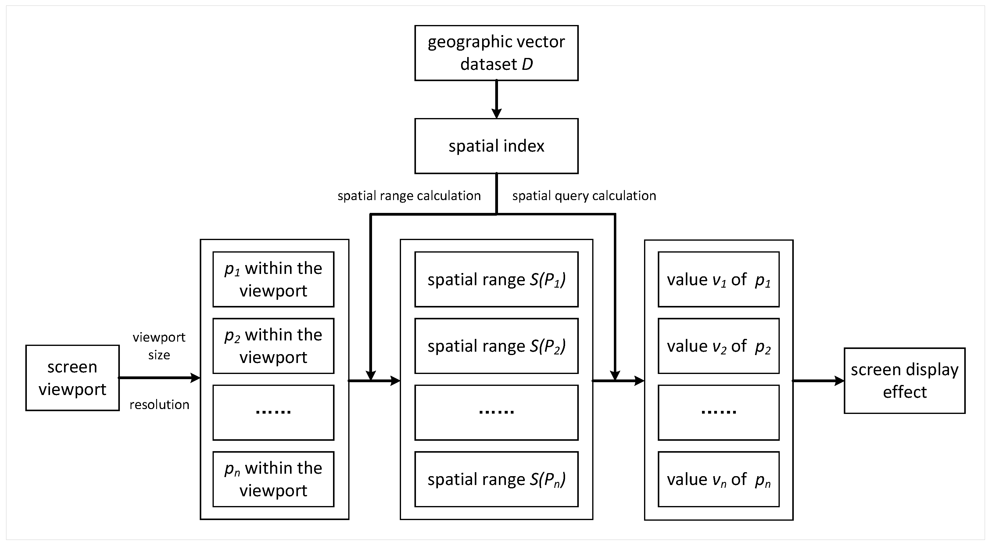
3.1. Viewport Generalization Visualization Model

The key ideas of the viewport generalization visualization model (VGVM) of geographic vector data are introduced in this section. Traditional geographic vector data visualization methods generally adopt a data-driven model—that is, starting from each geographic vector feature, the visualization results under a given resolution viewport are analyzed and calculated; then, the visualization results of all geographic vector features are superimposed, combined, and outputted. By summarizing the process of traditional methods, we propose a general processing model of traditional geographic vector data visualization methods, which can be expressed by Equation (1). In the equation, d i is a vector feature of the geographic vector dataset D within the viewport, N is the number of features, V ( D ) is the result of the visualization processing of D, M ( . ) is a plotting function of vector features, and F 1 F 2 F k represents the K-connected analytical processing functions. The meaning of the equation is as follows: For each vector feature in the dataset, K analysis processing operations are executed in sequence and associated to obtain the analysis processing result of the feature, and then the results are plotted. Finally, the plotted results of all vector features are aggregated to obtain the final visualization result V ( D ) .
V ( D ) = i = 1 N M [ F 1 F 2 F k ( d i ) ] , D = ( d i | i = ( 1 , , N ) )
Assuming that the average cost of analyzing each vector feature is A and the average number of drawn pixels for visualizing the analysis results of each vector feature is P, the computational complexity of Equation (1) can be expressed as Equation (2).
O [ N × ( A × K + P ) ]
We observe that the visualization of geographic vector data is achieved by calculating the display value of each pixel within the viewport. According to Equation (1), when a pixel is hit by multiple geographic vector features, its display value may be computed several times; thus, a large number of redundant calculations are generated.
Therefore, this paper designs a visualization model from the viewport perspective, whereby the display values of image pixels are quickly calculated by combining multiple geographic vector features within the viewport pixel range, as shown in Equation (3). In the equation, D is the geographic vector data, p i is the pixel with the viewport, C is the total number of viewport pixels, and R ( p i ) is a general calculation function of geographic vector features that can be designed in different forms. In Equation (4), a binarization design of R ( P i ) is shown, the core of which is the comprehensive calculation of the geographic vector features in the spatial range corresponding to image pixel p i ; when there are no geographic vector features in the spatial range corresponding to image pixel p i , the pixel value is 0. Conversely, when there are geographic vector features in the spatial range, the pixel value is 1. At the same time, as in Equation (5), R ( p i ) can also be designed as a function of the number of vector features in the corresponding spatial range of p i —that is, a function related to the density distribution of geographic vector data.
V ( D ) = i = 1 C R ( p i )
R ( p i ) = 0 S ( p i ) D = ϕ 1 S ( p i ) D ϕ
R ( p i ) = F ( | S ( p i ) D | )
As can be seen from the above equation, the visualization result V ( D ) of the dataset D has been converted from relying on the plotted value of each vector feature d i (Equation (1)) to relying on the intersection result of the corresponding spatial range of the image pixel p i with D (Equation (3)). Meanwhile, the computational complexity of Equation (3) mainly comes from the computational complexity of R ( p i ) . From Equation (4), R ( p i ) can be regarded as a spatial topology intersection operation. Then, tree indexing can be used, and the computational complexity of R ( p i ) in Equations (4) and (5) is generally O ( log N ) . The overall complexity of VGVM is shown as Equation (6). It can be seen that the cost is related to C and N. C is the total number of pixels within the viewport, which can be regarded as a constant, and its value is related to the size of the viewport. In currently used visualization devices, C is generally no more than a million in magnitude. N is the total number of vector features.
O ( C × log N )
Compared with Equation (2), the VGVM has performance advantages. First, when N is large, the total calculation time of VGVM, as shown in Equation (6), is less than that of the data-driven model. Second, as N increases, the complexity of Equation (2) increases linearly, while the complexity of Equation (6) increases by O ( 1 / N ) . When N is very large, the growth tends to zero. Furthermore, if we design a reasonable index structure to further improve the solving speed of S ( p i ) D in Equation (4), it will have better performance for BGVD visualization. In this process, in order to further improve the solving speed in Equation (4), a specific spatial index structure can be designed to rapidly generate pixel display values. The basic flow of the visualization strategy supporting VGVM is shown in Figure 1.

3.2. Viewport Pixel Quadtree Index Structure

In VGVM, the issue of plotting geographic vector features is transformed to the issue of querying hit vector features in the spatial range corresponding to display pixels; then, the display values of pixels are calculated according to the query results. The time-consuming part mainly comes from the process of querying vector features according to the spatial range of the pixel. To accelerate this process, we design a viewport pixel quadtree (VPQ) for display pixels.

3.2.1. Structure Design of VPQ

Quadtree divides spatial regions from two spatial dimensions into four equal rectangular subregions; then, it divides each subregion into four recursive subregions until the set depth is reached [25]. In order to be compatible with online geographic information applications, we take the Web Mercator projection [26] of global geographic space as the description space of geographic vector data, and perform the recursive decomposition of the spatial range based on quadtree. The projection takes the equator as the central latitude, the prime meridian as the central longitude, and the intersection of the two lines as the origin, and the longitude lines are parallel to each other and equally spaced. The projection does not include part of the north and south poles, and the overall projection area is square to facilitate the use of quadtree organization.
In the design of index structure, if the spatial range of the index node is aligned with the spatial range represented by the pixel, the spatial range that affects the pixel value can be quickly retrieved and the value generated. Accordingly, the index structure of VPQ is shown in Figure 2. The whole VPQ is composed of isomorphic index nodes. Each index node contains five parts:
(1)
G e o C o d i n g : The unique identification coding of the node. In order to speed up the spatial intersection calculation efficiency, the node coding adopts Geohash coding.
(2)
B B O X : The spatial range of the node.
(3)
C o u n t : The number of geographical vector features contained in the node.
(4)
C n o d e s : Pointers to the four children of the node.
(5)
L e v e l : The depth of the node in VPQ.
The index range of the root node of VPQ is the global geographic spatial range, and also serves as the general entrance of spatial range queries corresponding to the pixel. For branch nodes, if the four subregions of the node spatial range contain geographic vector features, the left-upper node (LUNode), right-upper node (RUNode), left-bottom node (LBNode), and right-bottom node (RBNode) pointing to the upper left, upper right, lower left, and lower right regions, respectively, of the spatial range of the parent node are created after division, and are arranged in accordance with the z-order spatial filling curve. For leaf nodes, if the node exists, this means that the node contains geographic vector features.

3.2.2. Construction Method of VPQ

The core of the VPQ index is to analyze the intersection between geographic vector features and the spatial range corresponding to the VPQ index node, so as to determine the visual mode of the viewport pixels corresponding to the index node. Geographic vector data can be geometrically divided into three types: point, line, and polygon. According to the characteristics of these three features, we design a judgment algorithm to determine the relationship between geographical vector features and index nodes in Algorithm 1. In the algorithm, p . t y p e is the type of the geographic vector feature, B B o x is the spatial range represented by a rectangle containing two diagonal points, and i n t e r s e c t and c o n t a i n are spatial topology judgment operations.
Algorithm 1: BBOXIntersectedGeometry: determine the intersection relationship between spatial range and geographic vector features.
  input: spatial range rectangle B B o x , geographic vector feature p.
  output: True: intersection; False: non-intersection
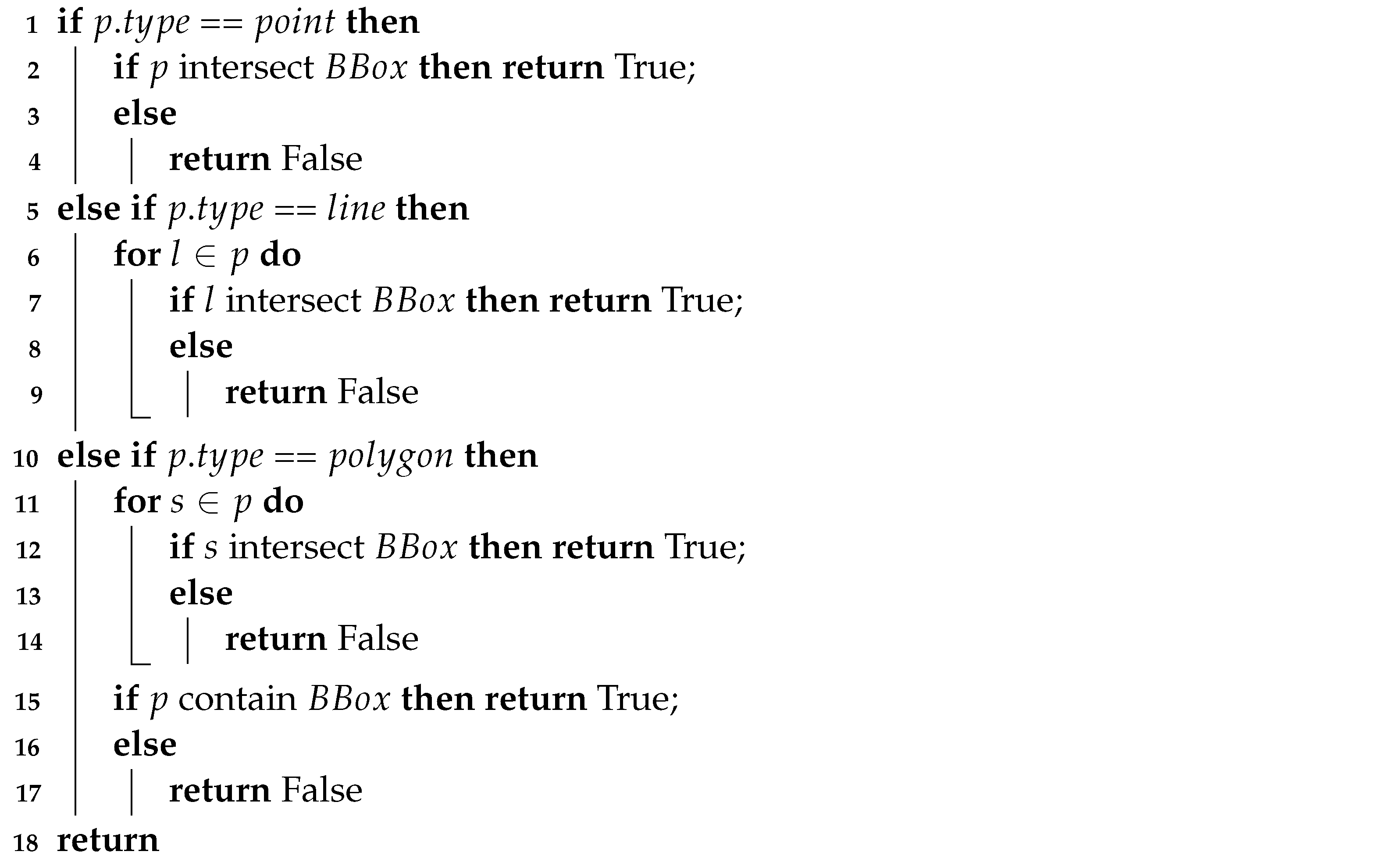
Applsci 12 07710 i001
The core idea is that, for point features, the rectangle corresponding to the index node and point is directly used to judge the intersection. For line and polygon data, each simple line segment forming the boundary of line and polygon features is judged. As long as there is a line segment intersecting with the rectangular spatial range of the index node, the vector feature can be considered to have intersected with the index node. For polygon features, there is also a case to deal with; that is, although the polygon boundary does not intersect with the index node, the index node is inside the polygon feature, which is also judged to intersect with the index node. In the above cases, the intersection judgment can be summarized as the intersection of a point and a simple line segment with a rectangular region, which can be quickly judged by geometric computational methods.
According to the structure design of the VPQ index and the determination algorithm of the intersecting relationship between geographic vector features and index nodes, we designed the construction process of VPQ index as follows:
(1)
Create the root node of the VPQ index according to the global spatial range and set the maximum depth of the VPQ index.
(2)
Perform the necessary coordinate transformation and perform the following Steps 3 to 6 for each feature in the input geographic vector data.
(3)
Take the VPQ root node as the current index node R.
(4)
The counter, C o u n t , of the R increases by 1. If the level, l e v e l , does not reach the maximum depth, the spatial range, B B o x , of R is divided into four spatial subranges, S l u (upper left), S r u (upper right), S l b (lower left), and S r b (lower right), and algorithm 1 is adopted to test the intersection between the current geographic vector feature p and the four subregions one by one. If it intersects, the pointer will be positioned at the child node. If the child node does not exist, the child node of the corresponding region will be generated.
(5)
For each newly positioned child node, take it as the new current node R and skip to Step 4 to continue the execution.
(6)
Continue until there are no new positioning nodes.
According to the above process, all regions containing geographic vector data have corresponding nodes in the VPQ index, and the number of geographic vector features is reflected in the Count attribute of the node. Any region without geographic vector data has no corresponding node in the VPQ index.

3.3. VPQTree-Based Preview Algorithm of BGVD

In the VGVM of geographic vector data, the issue of geographic vector data visualization is transformed into the query of matching vector features in the spatial range corresponding to screen pixels. The judgment criterion for calculating pixel display values is as follows: if the number of vector features within the spatial range corresponding to the pixel is greater than the set threshold, the pixel value will be generated; otherwise, no pixel value will be generated. In the VPQ index constructed from geographic vector data, the index nodes that hit the vector features in the spatial range are created and the spatial range of the index nodes in the VPQ index is mapped to the spatial range corresponding to the pixel. Therefore, with the support of the VPQ index, the issue of geographic vector data visualization can be transformed to query whether the index node corresponding to the pixel to be calculated exists in the VPQ index.
In this section, we propose a VPQTree-based preview algorithm of BGVD (VPQP) to generate the pixel display value in the viewport for the final preview display effect. The main process is as follows: in the process, “partial matching” means that the encoding of the child node of query node S is consistent with the corresponding prefix digit of the encoding of the pixel, and “equal matching” means that the encoding of the child node of query node S is completely consistent with the encoding of the pixel.
(1)
Calculate the corresponding spatial range of the pixel according to the pixel number.
(2)
Encode the spatial range of the pixel, and set the number of encoding times to 8 at the tile level to which the pixel belongs, so as to obtain the Geohash encoding of the pixel.
(3)
Start the query from the root node of VPQ index, and take the root node as the current query node S.
(4)
Match the Geohash encoding of the pixel with the encoding of the child node of query node S.
(5)
If the two encodings exhibit “partial matching”, the last two digits of the matching result are used: if they are“00”, the pointer is positioned to the lower left child node; if they are “10”, the pointer is positioned to the lower right child node; if they are “01”, the pointer is positioned to the upper left child node; and if they are “11”, the pointer is positioned to the upper right child node. Otherwise, the pixel value does not need to be generated and the process ends.
(6)
Take the newly positioned index node as the new current query node S and skip to Step 4 to continue the execution.
(7)
The pixel value is generated until the encoding of the child node of query node S and the encoding of the pixel exhibit “equal matching”.
The VPQP algorithm of geographic vector data is shown as Algorithm 2. In the algorithm, ← is the assignment operation; R T is the stack, which is a data structure that follows the “first in, first out” rule; R a n g e ( . ) is the function of obtaining the spatial range of the pixel; G e o h a s h ( . ) is the function of obtaining the binary Geohash encoding of a spatial range; M a t c h ( . ) is the function that obtains the same substring of both encodings; and S . C n o d e s [ l u / r u / l b / r b ] represent the four children of node S, respectively.
Algorithm 2: The VPQP algorithm of geographic vector data.
  input: VPQ index V P Q T r e e , pixel P, tile level z, threshold of vector features δ .
  output: True: the value of pixel P is generated; False: the value of pixel P is not generated.
Applsci 12 07710 i002

4. Experiment

4.1. Experiment Settings

The experiment was carried out on a cluster system consisting of four high-performance computers as computing nodes. The four computing nodes were connected via a 10-gigabit Ethernet network. Each node had 32 CPUs and 512 GB of memory. Experimental data were from the open-source projects OpenStreetMap [3] and OpencellID [27]. Some data with more than 100 million geographical vector features were selected to verify the efficiency of the proposed method. The experimental data configuration is shown in Table 1.
The algorithm code in this paper is based on C++11, and the external function libraries that were called include Proj 4.9.2, Mpich 3.3.2, Redis 3.2.12, Libpng 1.2.59, Crow 0.3, etc. The software used for performance comparison relies on libraries such as Boost C++ 1.72, Hadoop 2.9.2, Spark 2.3.3, SpatialHadoop 2.4.2, GeoSpark 1.2.0, and Mapnik 3.0.22. In the experiment, VPQ indexes were established for each dataset, which were saved as index files in the file system and deployed in each computing node in the cluster environment.

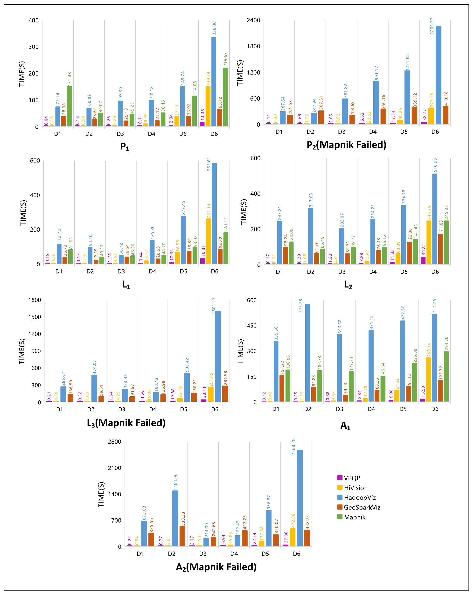
4.2. Comparative Analysis of Geographic Vector Data Visualization Performance

The proposed method was compared and analyzed with the four existing geographic vector visualization methods, namely, HadoopViz [18], GeoSparkViz [20], Mapnik, and HiVision [21]. In order to verify the advantages of the method compared with traditional data-oriented methods, the first three most-representative data-driven geographic vector data visualization methods were selected, which adopt high-performance parallel computing architecture to accelerate the realization of big geographic vector data visualization and have good performance. HadoopViz is implemented based on Hadoop, and GeosparkViz is implemented based on Spark, a distributed memory computing framework. These two methods both provide good load balancing to improve the overall computing performance. For the given geographic vector data, they can quickly generate visualization results in the form of map tiles in a distributed parallel manner. Mapnik is a high-performance mapping tool for a wide range of applications, allowing the rapid mapping output of geographic vector data with a given mapping spatial range and style. At the same time, in order to verify the performance improvement of this method compared with our previous work, we also compared the visualization algorithm proposed in our previous work, HiVision, which is a high-performance visualization algorithm of geographic vector data rasterization based on the MPI computing framework.
In the experiment, the global tile pyramid division model was used to organize the visualization results, and six scenes of drawing scale were designed from small to large (Table 2). First, the experimental data were drawn on a 4096 × 4096 canvas; then, the canvas was divided along the tile pyramid model layer by layer, with each layer being four times larger than the previous layer.
We used the MPI + OpenMP hybrid parallel method to execute the proposed algorithm. According to the total number of CPU cores in the experimental configuration, 128 MPI task processes were started in the cluster environment, and 2 OpenMP threads were started in each MPI task process for the parallel computation of the preview drawing in a given area. Comparative results are shown in Figure 3.
From the experimental results, firstly, it can be seen that among the geographic vector data visualization methods involved in the comparison, GeoSparkViz takes less time than the other three methods for drawing scenes with a larger number of pixels. HiVision takes less time than the other three methods for drawing scenes with a smaller number of pixels. Compared with the existing methods, the plotting time of the proposed VPQP algorithm is much smaller than the existing methods on all datasets and in all drawing scenes, and for the billion-scale datasets, P 2 , L 3 , and A 2 , the plotting time of the algorithm is only 10.4% (=38.77 s ÷ 373.16 s), 15.2% (=38.11 s ÷ 251.43 s), and 8.8% (=37.86 s ÷ 432.23 s), respectively, indicating that the proposed algorithm has excellent plotting performance. Secondly, with the increase in pixel size in scenes D1 to D6, the rendering time of the existing method increases sharply. Compared with this, the increasing trend of the rendering time of the VPQP algorithm is small, indicating that the algorithm has low computational complexity. Then, we observe that as the size of the dataset grows from L 1 to L 3 , the difference in plotting time between the three datasets under each plotting scene is small, indicating that the VPQP algorithm has the property of being insensitive to data size and is suitable for the preview visualization of BGVD. Finally, the drawing time of the VPQP algorithm in drawing scenes D1 and D2 is less than 1 s, which indicates that the algorithm has good performance in supporting real-time previews. In practice, the data preview operation usually follows a general to local process, and the image size within the screen is usually smaller than the image size in the above drawing scenes, which shows that the proposed method has better performance in supporting the interactive real-time visualization of BGVD compared with existing visualization methods.

4.3. Analysis of Real-Time Preview Performance

To verify the ability of the proposed VPQP algorithm to support the real-time preview of BGVD, we randomly selected 3072 × 2048 drawing areas in each experimental scene in Table 2 and analyzed the average drawing time of each dataset, as shown in Table 1, in order to observe the delay performance of the proposed VPQP algorithm for data preview under the viewport resolution of current mainstream display devices.
In this experiment, we started 64 MPI processes, each containing four OpenMp threads for generating preview visualization results. We conducted 20 random experiments for each dataset according to the above settings, and then counted the preview latency of the generated results. The experimental results are shown in Figure 4. In Figure 4, the bottom line represents the smallest preview latency, the top line represents the largest preview latency, and the symbol “×” represents the average preview latency in the repeated experiments. Since single experiments have a certain degree of chance, we selected the average value of the preview latency for analysis. The results show that the average preview latency of all datasets in the 3072 × 2048 region is between 1 s and 1.5 s, which can support real-time previews in terms of human–computer interactions. We also observe that although the scale of each experimental dataset in Table 1 is relatively different, their average preview drawing latency does not differ by much, indicating that the proposed method is not sensitive to data size. This advantage provides good interaction stability and data scale adaptation when previewing BGVD.

5. Conclusions and Future Work

Aiming to solve the problem of the real-time visualization of BGVD, this paper explores a new method that takes the viewport pixel as the visual computing unit, analyzes the spatial relationship between the spatial range corresponding to the viewport pixel and geographic vector data, and then judges the pixel value according to the results in terms of the spatial relationship. The proposed method shifts the dependence of the visualization calculation cost on the data scale to the viewport image pixel scale. Based on the model, the viewport pixel quadtree index and the VPQ-based real-time visualization algorithm are proposed. Experiments on billion-scale data show that the proposed method has a more than ten times greater improvement in performance compared with the existing optimal methods, and achieves a real-time computation and visualization preview for BGVD. Furthermore, the visualization results of the proposed method are all temporarily stored in memory and do not require external memory space, which is more advantageous in terms of resource consumption cost than the existing visualization methods that require a large amount of external memory space to temporarily store tile data.
In the follow-up study, combined with our previous exploration and experimental attempts, the adaptability of the proposed method to different viewport resolutions needs to be further studied. The VPQ-based visualization method of BGVD has obvious performance advantages when the viewport resolution is relatively small, especially when the viewport covers all features of the geographic vector dataset, and the pixel scale of the viewport is much smaller than that of the geographic vector data. However, when the viewport resolution is relatively large and the size of the viewport pixels is larger than the size of the geographic vector data, the performance of the existing methods is inferior. Therefore, it is necessary to further study the adaptability of this method to different viewports.

Author Contributions

Conceptualization, L.C. and Z.L.; methodology, L.C. and Z.L.; software, Z.L. and M.M.; formal analysis, L.C. and Z.L.; resources, M.M.; writing—original draft preparation, L.C. and Z.L.; writing—review and editing, Z.L., M.M. and L.C.; visualization, Z.L. and M.M.; project administration, L.C.; funding acquisition, L.C. and M.M. All authors have read and agreed to the published version of the manuscript.

Funding

This research was funded by the National Natural Science Foundation of China under Grant Nos. 41971362 and 42101432 and the Natural Science Foundation of Hunan Province under Grant Nos. 2019JJ50718 and 2022JJ40546.

Data Availability Statement

All data used in experiment are from openstreetmap and can be accessed with the following link: https://www.openstreetmap.org/ (accessed on 25 June 2022).

Conflicts of Interest

The authors declare no conflict of interest.

Abbreviations

The following abbreviations are used in this manuscript:
GISgeographic information system
VPQviewport pixel quadtree
VGVMviewport generalization visualization model

References

  1. Zhou, C. Prospects on pan-spatial information ssystem. Prog. Geogr. 2015, 34, 129–131. [Google Scholar] [CrossRef]
  2. Robinson, A.C.; Demšar, U.; Moore, A.B.; Buckley, A.; Jiang, B.; Field, K.; Kraak, M.J.; Camboim, S.P.; Sluter, C.R. Geospatial big data and cartography: Research challenges and opportunities for making maps that matter. Int. J. Cartogr. 2017, 3, 32–60. [Google Scholar] [CrossRef] [Green Version]
  3. OPENSTREETMAP. Openstreetmap. Available online: https://www.openstreetmap.org/ (accessed on 25 June 2022).
  4. Natural Resources Ministry of China. Bulletin of the Third National Land Survey. Available online: http://www.mnr.gov.cn/dt/ywbb/202108/t20210826_2678340.html (accessed on 25 June 2022).
  5. Monmonier, M. Strategies for the Visualization of Geographic Time-Series Data. In Classics in Cartography; Wiley: Hoboken, NJ, USA, 2011; pp. 55–72. [Google Scholar] [CrossRef]
  6. Ghosh, S. Interactive Visualization for Big Spatial Data. In Proceedings of the 2019 International Conference on Management of Data, Amsterdam, The Netherlands, 30 June–5 July 2019; Association for Computing Machinery: New York, NY, USA, 2019; pp. 1826–1828. [Google Scholar] [CrossRef]
  7. Li, S.; Dragicevic, S.; Castro, F.A.; Sester, M.; Winter, S.; Coltekin, A.; Pettit, C.; Jiang, B.; Haworth, J.; Stein, A.; et al. Geospatial big data handling theory and methods: A review and research challenges. ISPRS J. Photogramm. Remote. Sens. 2016, 115, 119–133. [Google Scholar] [CrossRef] [Green Version]
  8. Çoltekin, A.; Griffin, A.L.; Slingsby, A.; Robinson, A.C.; Christophe, S.; Rautenbach, V.; Chen, M.; Pettit, C.; Klippel, A. Geospatial information visualization and extended reality displays. In Manual of Digital Earth; Springer: Singapore, 2020; pp. 229–277. [Google Scholar]
  9. Zhu, Q.; Fu, X. The Review of Visual Analysis Methods of Multi-modal Spatio-temporal Big Data. Acta Geod. Cartogr. Sin. 2017, 46, 1672–1677. [Google Scholar] [CrossRef]
  10. Cruz, I.F.; Ganesh, V.R.; Caletti, C.; Reddy, P. GIVA: A Semantic Framework for Geospatial and Temporal Data Integration, Visualization, and Analytics. In Proceedings of the 21st ACM SIGSPATIAL International Conference on Advances in Geographic Information Systems, Orlando, FL, USA, 5–8 November 2013; Association for Computing Machinery: New York, NY, USA, 2013; pp. 544–547. [Google Scholar] [CrossRef]
  11. Yao, X.; Li, G. Big spatial vector data management: A review. Big Earth Data 2018, 2, 108–129. [Google Scholar] [CrossRef]
  12. Wan, L.; Huang, Z.; Peng, X. An Effective NoSQL-Based Vector Map Tile Management Approach. ISPRS Int. J. -Geo-Inf. 2016, 5, 215. [Google Scholar] [CrossRef] [Green Version]
  13. Guo, M.; Guan, Q.; Xie, Z.; Wu, L.; Luo, X.; Huang, Y. A spatially adaptive decomposition approach for parallel vector data visualization of polylines and polygons. Int. J. Geogr. Inf. Sci. 2015, 29, 1419–1440. [Google Scholar] [CrossRef]
  14. Li, J.; Wu, H.; Yang, C.; Wong, D.W.; Xie, J. Visualizing dynamic geosciences phenomena using an octree-based view-dependent LOD strategy within virtual globes. Comput. Geosci. 2011, 37, 1295–1302. [Google Scholar] [CrossRef]
  15. Laura, J.; Rey, S.J. Improved Parallel Optimal Choropleth Map Classification. In Modern Accelerator Technologies for Geographic Information Science; Shi, X., Kindratenko, V., Yang, C., Eds.; Springer: Boston, MA, USA, 2013; pp. 197–212. [Google Scholar] [CrossRef]
  16. Tang, W. Parallel construction of large circular cartograms using graphics processing units. Int. J. Geogr. Inf. Sci. 2013, 27, 2182–2206. [Google Scholar] [CrossRef]
  17. Eldawy, A.; Mokbel, M.F.; Alharthi, S.; Alzaidy, A.; Tarek, K.; Ghani, S. SHAHED: A MapReduce-based system for querying and visualizing spatio-temporal satellite data. In Proceedings of the 31st International Conference on Data Engineering, Seoul, Korea, 13–17 April 2015; pp. 1585–1596. [Google Scholar] [CrossRef] [Green Version]
  18. Eldawy, A.; Mokbel, M.F.; Jonathan, C. HadoopViz: A MapReduce framework for extensible visualization of big spatial data. In Proceedings of the 32nd International Conference on Data Engineering (ICDE), Helsinki, Finland, 16–20 May 2016; pp. 601–612. [Google Scholar] [CrossRef]
  19. Yu, J.; Sarwat, M. GeoSparkViz: A cluster computing system for visualizing massive-scale geospatial data. VLDB J. 2021, 30, 237–258. [Google Scholar] [CrossRef]
  20. Yu, J.; Tahir, A.; Sarwat, M. GeoSparkViz in Action: A Data System with Built-in Support for Geospatial Visualization. In Proceedings of the 35th International Conference on Data Engineering (ICDE), Macao, China, 8–11 April 2019; pp. 1992–1995. [Google Scholar] [CrossRef]
  21. Ma, M.; Wu, Y.; Ouyang, X.; Chen, L.; Li, J.; Jing, N. HiVision: Rapid visualization of large-scale spatial vector data. Comput. Geosci. 2021, 147, 104665. [Google Scholar] [CrossRef]
  22. Ma, M.; Yang, A.; Wu, Y.; Chen, L.; Li, J.; Jing, N. DiSA: A Display-driven Spatial Analysis Framework for Large-Scale Vector Data. In Proceedings of the 28th International Conference on Advances in Geographic Information Systems, Seattle, WA, USA, 3–6 November 2020; pp. 147–150. [Google Scholar] [CrossRef]
  23. Liu, Z.; Chen, L.; Yang, A.; Ma, M.; Cao, J. HiIndex: An Efficient Spatial Index for Rapid Visualization of Large-Scale Geographic Vector Data. ISPRS Int. J. -Geo-Inf. 2021, 10, 647. [Google Scholar] [CrossRef]
  24. Chen, L.; Liu, Z.; Ma, M. HiVecMap: A parallel tool for real-time geovisualization of massive geographic vector data. SoftwareX 2022, 19, 101144. [Google Scholar] [CrossRef]
  25. Samet, H. The quadtree and related hierarchical data structures. ACM Comput. Surv. 1984, 16, 187–260. [Google Scholar] [CrossRef] [Green Version]
  26. Battersby, S.E.; Finn, M.P.; Usery, E.L.; Yamamoto, K.H. Implications of web Mercator and its use in online mapping. Cartogr. Int. J. Geogr. Inf. Geovis. 2014, 49, 85–101. [Google Scholar] [CrossRef]
  27. OPENCELLID. OpenCellID. Available online: https://opencellid.org/ (accessed on 25 June 2022).
Figure 1. Viewport generalization visualization model of geographic vector data.
Applsci 12 07710 g001
Figure 2. Structure of viewport pixel quadtree.
Applsci 12 07710 g002
Figure 3. Comparative results of the rendering performance of different methods.
Applsci 12 07710 g003
Figure 4. Real-time performance evaluation of the proposed method.
Applsci 12 07710 g004
Table 1. Configuration of experimental data.
DatasetTypeRecordsSize
P 1 : OpenCeilliD cell tower locationspoint40,719,47840,719,478 points
P 2 : OSM all points on the planetpoint2,682,401,7632,682,401,763 points
L 1 : OSM water areas boundarieslinestring9,211,000376,208,235 segments
L 2 : OSM roadslinestring72,336,396717,048,198 segments
L 3 : OSM all linestrings on the planetlinestring106,268,5541,573,469,984 segments
A 1 : OSM buildingspolygon114,839,692804,028,282 edges
A 2 : OSM all polygons on the planetpolygon181,772,6922,077,524,465 edges
Table 2. The design of drawing scenes.
Scene IDPixel Size
D 1 4096 × 4096
D 2 8192 × 8192
D 3 16,384 × 16,384
D 4 32,768 × 32,768
D 5 65,536 × 65,536
D 6 131,072 × 131,072
Publisher’s Note: MDPI stays neutral with regard to jurisdictional claims in published maps and institutional affiliations.

