Abstract
Plastic pollution, largely perceived by the public as a major risk factor that strongly impacts sea life and preservation, has an even higher negative impact on terrestrial ecosystems. Indeed, quantitative data about plastic contamination on agricultural soils are progressively emerging in alarming ways. One of the main contributors to this pollution involves the mismanagement of agricultural plastic waste (APW), i.e., the residues from plastic material used to improve the productivity of agricultural crops, such as greenhouse covers, mulching films, irrigation pipes, etc. Wrong management of agricultural plastics during and after their working lives may pollute the agricultural soil and aquifers by releasing macro-, micro-, and nanoplastics, which could also enter into the human food chain. In this study, we aimed to develop a methodology for the spatial quantification of agricultural plastics to achieve sustainable post-consumer management. Through an inductive approach, based on statistical data from the agricultural census of the administrative areas of the Italian provinces, an agricultural plastic coefficient (APC) was proposed, implemented, and spatialized in a GIS environment, to produce a database of APW for each type of crop. The proposed methodology can be exported to other countries. It represents valuable support that could realize, in integration with other tools, an atlas of agricultural plastics, which may be a starting point to plan strategies and actions targeted to the reduction of the plastic footprint of agriculture.
1. Introduction
Soil represents one of the fundamental elements for any type of terrestrial ecosystem; it is an essential asset for human life. Ensuring the preservation/recovery of soil ecosystem health is one of the most important challenges that has emerged in recent decades. This is one of the key aspects of the Sustainable Development Goals and one of the objectives of the European Green Deal [1,2]. Among the many strategies implemented by various international organizations, the Soil Health Mission aims to ensure that, by 2030, 75% of soils are healthy and able to provide ecosystem services that are essential to human life [3]. Indeed, the soil issue is cross-cutting and connected to the other objectives of the European Green Deal related to climate, biodiversity, pollution, agri-food system sustainability, and ecosystem resilience. Within the imagined strategy, one of the specific objectives is to protect the soil ecosystem from excessive plastic pollution [4].
Plastic pollution is a global issue that also affects food security due to its presence in most aquatic and terrestrial ecosystems [5]. This type of pollution is so ubiquitous that it was recently discovered in human blood [6]. Since the 1960s, global production of plastics has increased 20-fold, exceeding 300 million tons in 2015; it is predicted to double in the next 20 years [7,8]. Therefore, it has become imperative to study and understand how this increase in plastics will impact severely compromised ecosystems. Many previous studies were conducted on the impacts of plastic pollution on aquatic ecosystems [9], but little has been investigated so far on terrestrial habitats [10,11].
Agricultural activities are among the most important sources of plastic in the soil; they are often underestimated as they are difficult to quantify [12,13]. This is because agricultural productivity and sustainability are substantially influenced by the use of plastic polymers in various forms and structures. Their main benefits are that they are lightweight and cheap and, hence, can be used in very large volumes in agricultural activities [14]. Mulch films, polymer-coated soil additives, seeds, greenhouses, polytunnels, and silage product packaging are made of plastic; they are used in almost all agricultural activities [15].
As per the common agricultural policy [16], one of the most important topics to be addressed is activating the sustainable management of plastics in agriculture, to reduce the negative impacts of the release of micro- and nanoplastics in the soil [17]. The release of plastic residues into farmland and their influences on soil health and long-term crop production are still not clear (Zhang et al.). For example, one of the first analyses was by Phiel et al. [18] in southeast Germany, where the macro- and microplastic pollution on agricultural fields were quantified with values of around 200 macroplastics (pieces/hectares) and between 0.34 and 0.36 microplastics (particles/kilogram of the dry weight of soil). A more recent case study was carried out in Taiwan [19], where differences in the amounts of microplastics (12–117 items/m2) were found between farmlands near the road (more than three times) compared to those more isolated.
The problem of plastic pollution in agriculture is linked not only to the large quantities used but also to poor and inefficient management at the farmland level and the level of competent authorities responsible for agricultural plastic waste (APW) [8]. The lack or inefficiency of agricultural plastic waste management and recycling systems in most European countries means that illegal disposal practices often occur [20,21].
The first step toward proper management of APW and, therefore, reducing their environmental footprint, is to quantify them, i.e., to implement different post-use sustainable management actions. The techniques are different, but surely the most used methodologies are based on a GIS approach [22,23,24].
In the present paper, to develop useful methodologies that realize the digital atlas of agricultural plastics, an inductive (i.e., bottom-up) approach is proposed based on statistical data and the relevant index of the potential use of plastic material for cultivated crops in a study area. This approach has the same general objective, but it is different from the deductive approach (i.e., top-down) presented in the first part of the work already published [25], in which a deductive methodology was implemented by exploiting satellite index images and orthophoto classifications [26]. In this case, the methodology is based on the analysis and processing of statistical data from the agricultural census based on a well-defined administrative scope. Data (in terms of hectares on the different crops examined) were correlated with data on the types and quantities of plastics used for the crops derived from questionnaires proposed to various producers and agricultural associations [27]. In this way, it was possible to quantify potentially the APW amount in terms of weight (tons per year) for each administrative area considered. The data were processed in a GIS environment since, in addition to spatializing different types of geoinformation [28], they allowed for rapid operations and conversions in an immediate manner [29]. The approach adopted here is similar to the one used by Briassoulis et al. [30], but the data (referred to Italy) were updated and calculated in more detail, with support from Italian experts on protected cultivations (farmer associations/organizations/cooperatives).
Therefore, in previous work [25], an additional geomatics methodology is provided, which is accurate but at the same time easy to apply on a large-scale and in other administrative contexts, in order to realize (in the future) a complete atlas of plastics at a European scale, which can be used as a tool for planning and monitoring (at land level) the environmental footprint reductions of several agricultural activities. Indeed, the methodology, integrated with the work already proposed [25], can be a tool to support public administration to estimate APW with some accuracy, with a reliable and spatially explicit database able to activate sustainable management strategies.
2. Materials and Methods
The proposed inductive approach is based on the elaboration and spatialization of statistical data, referring to an Italian administrative level, namely the provincial level (NUTS 3 region). This generalized level of analysis was necessary because, in Italy, agricultural census data are provided at the municipal level by the regions (NUTS 2 regions) every ten years; to date, the latest available data are those for 2010. Instead, the Italian Institute of Statistics [31] provides data every year at the provincial level [ISTAT; 2020]. Therefore, for the application of more recent data to carry out an updated evaluation of APW, we opted for the data at the provincial level for the year 2020.
2.1. Study Areas
Agriculture in Europe [32] is a sector dominated by small-scale farms: 65% have areas of less than 5 hectares and only 3% of farms in the European Union reach 100 hectares, working more than half of the utilized agricultural areas (UAAs). The structure of EU agriculture remains dominated by people over 60 years old. The ages of those individuals running the farms show that only 11% of managers are under 40 years old compared to a third (32%) who are 65 years old.
In this context, with just over 12 million hectares of land used, Italian agriculture accounts for over 12% of the sector’s turnover in the EU-27, confirming its position as the continent’s third largest agricultural economy after France (17% with 28 million hectares) and Germany (13% with 15 million hectares). One of the most important aspects of Italian agriculture is that a lot of plastic is used due to the high input of greenhouse cultivation. In 2020, more than 1.2 million hectares were cultivated in Italy for fruit and vegetable production, according to data from the Italian Institute of Agricultural Food Market Services (Ismea) published in April 2021, of which 39,000 hectares (or 3%) were allocated to greenhouse vegetable production [33].
Regarding greenhouse crops, in Italy, they are scattered all over the country, but the most representative areas are located from the north to the south, in Lombardia, Veneto, Liguria, Toscana, Lazio, Campania, Sicilia, and Sardegna (Figure 1). Greenhouses are particularly widespread along the sea coast, which has a mild winter climate [34].
Figure 1.
Localization of Italian provinces within the Mediterranean area (left) and the distribution of non-irrigated and permanently irrigated arable land according to Corine Land Cover 2018 (right).
2.2. Inductive Approach Procedure
The approach proposed in this paper is based on two distinct steps:
- (1)
- Realization of a coefficient to compute the amount of plastic (APCoeff) per year based on the vegetable crop areas (vineyards and orchards were not considered), starting from an approach proposed by Briassoulis et al. [30] and partly investigated by other authors [35,36];
- (2)
- Application and analysis (in a GIS environment) of the coefficient through spatial join operations to create a database of APW quantities for the different administrative areas considered.
Through these two steps, it was possible to make a preliminary estimate of the number of agricultural plastics expressed in tons per year, using data commonly produced by agricultural censuses and interviews with farmers. For this study, the reference was the census of the Italian National Institute of Statistics [37] with data from 2020; only some crops were considered (Table 1). The crops examined were those that required specific plastic structures during their production cycles and that represented a large part of Italian horticultural production.
Table 1.
List of crops used in this study and their acronyms used in the subsequent tables.
The first step was to retrieve data related to the types of crops examined. Data were selected from the national database and exported based on the area in cultivated hectares for each Italian province. Thanks to the ISTAT database [37], it is possible to perform a specific query by crop type and administrative area and export them in a spreadsheet, i.e., in raw comma-separated value (.CSV) format that is easy to manipulate in a GIS environment.
The second step involved a survey of the main producers and agricultural associations to whom, through a specific questionnaire, were asked for information about the use of plastics during the production cycle of the crops examined. Specifically, the following information was requested: type of plastic materials used, type of polymer, chemical–physical and mechanical characteristics, duration of use, and how they are managed before and after use.
In view of the types of crops considered, the plastic structures analyzed for the calculation of APCoeff were: plastic film of greenhouses, mulch sheets, and dripline. These structures were mainly used for crop protection from weathering, regulation of growing conditions, reduction of weeds, and reduction of water use [14]. Other plastic products, such as agrochemical containers and fertilizer bags, were not considered in this preliminary study. APCoeff (kg·m−2·years−1) for the plastic film was calculated according to the following formula):
where ρ is the density (kg m−3) of the product, as reported on the labels provided by manufacturers; Tk is the thickness (on the packaging, it is reported in μm, but it is necessary to convert it into meters); years refer to the plastic useful lifetime expressed in year(s); CACorr is a dimensionless correction factor [35], taking into account the increase or decrease of the material surface due to the different coverages with respect to the real cultivated surface. For example, the plastic film used to cover greenhouses extended on a larger area than the protected agricultural area—opposite to what often happens with the mulch film, as it covers only a portion of the cultivated surface. This correction factor is fundamental since the data on agricultural crops refer to the cultivated surface in general. The CAcorr is different for each crop and each type of plastic used. When it is greater than 1, it means that the crop needs more plastic in terms of surface area than is actually cultivated. If it is less than 1, the opposite is true. All CACorr values are reported in Table A1 in Appendix A.
APCoeff_film = (ρ · Tk · years−1) · CACorr
In addition, we should note that for some crops (melon and watermelon) the APCoeff_film was calculated for both greenhouses and tunnels (APCoeff_tunnel) used during the crop cycle. The formula is identical.
The APCoeff for the mulch sheet (APCoeff_mulch) was also calculated in the same way as the plastic film:
APCoeff_mulch = (ρ · Tk · years−1) · CACorr
Finally, for irrigation pipes, the APCoeff_irr was calculated on the basis of Equation (3). In this case, the density is expressed in kg per meter (kg·m−1) because the type of plastic product and the technical characteristics are different. In all the companies interviewed, irrigation pipes with the same characteristics in terms of plastic were used.
APCoeff_irr = (ρ · years−1) · CACorr
The sum of the contributions due to the different types of agricultural plastics defined the total amount of plastic waste for each specific crop (Equation (4)):
APCoeff_tot = APCoeff_film + APCoeff_mulch + APCoeff_irr
The Formulas (1)–(4) were modified from those proposed by other authors [23,30]. The indices were verified with literature data, direct communications from producers, and the University of Basilicata and University of Bari databases on the physical properties of agricultural plastics.
To clarify the methodology used to implement the calculation, Table 2 shows the calculation of only some types of crops as examples. Some crops, although different from each other, have cultivation cycles, such that farmers use the same types of plastic; for this reason, the values are the same.
Table 2.
Examples of different APCoeffs calculated for some crops.
Regarding the statistical data in the database—those on the individual cultivated areas for each province are reported in Appendix A. To provide an overall view, all the areas (in hectares) of the crops analyzed were summed up within an initial mapping of the cultivated areas, as shown in Figure 2.
Figure 2.
Map of cultivated areas in hectares for each Italian province. Values represent the total hectares of crops, shown in Table 1.
Subsequently, using the basic tools of the QGIS software, a join was made between the APCoeff data and the administrative areas in order to map the quantities of APW through the product between the cultivated area for each type of crop and the calculated APCoeff. The interoperability between tabular data in .CSV format and vector data in QGIS guarantees simplicity and immediacy of use. Moreover, once the GIS project was set up, it is possible to make operations, analyses, and data interrogation in a consequential way [29].
3. Results and Discussions
The most important and fundamental datum for the management of plastics involves the types of polymer used. From the survey and interviews, it emerged that films and sheets consist of:
- -
- High-density polyethylene (PE-HD);
- -
- Low-density polyethylene (PE-LD);
- -
- Polyvinyl chloride (PVC).
Demonstrating the need to activate intelligent and geospatial management of plastics—most of the interviewees did not have a strategy for the storage of materials and, therefore, disposal was not organized. Waste management is a central issue in all works concerning plastic pollution in rural areas, so it is increasingly necessary to study and develop tools and methodologies to address these problems [38].
Interviews were crucial because they allowed us to estimate the number of plastics that were impossible to detect remotely (via satellite or orthophotos) especially given their size, such as irrigation pipes or mulch, which, with the medium-resolution images commonly used for APW estimation [25,39], were impossible to classify. That being said, the analysis focused only on those crops for which it was possible to retrieve data from the sample of interviewees; therefore, the analysis may be considered only from a methodological point of view, since it does not yet include all crops grown in Italy. The calculated potential of APW represents only a proportion of the total agricultural plastic waste produced in Italy. This is because the flow of plastic products within the agricultural market is too scattered and, therefore, available data are extremely dispersed and often divergent. Once the GIS project is set up and the data are connected in .CSV format, it is possible to extrapolate all of the necessary data for a detailed analysis and for all of the following operations that can be useful for hypothetical waste management planning at the local and/or provincial level [40].
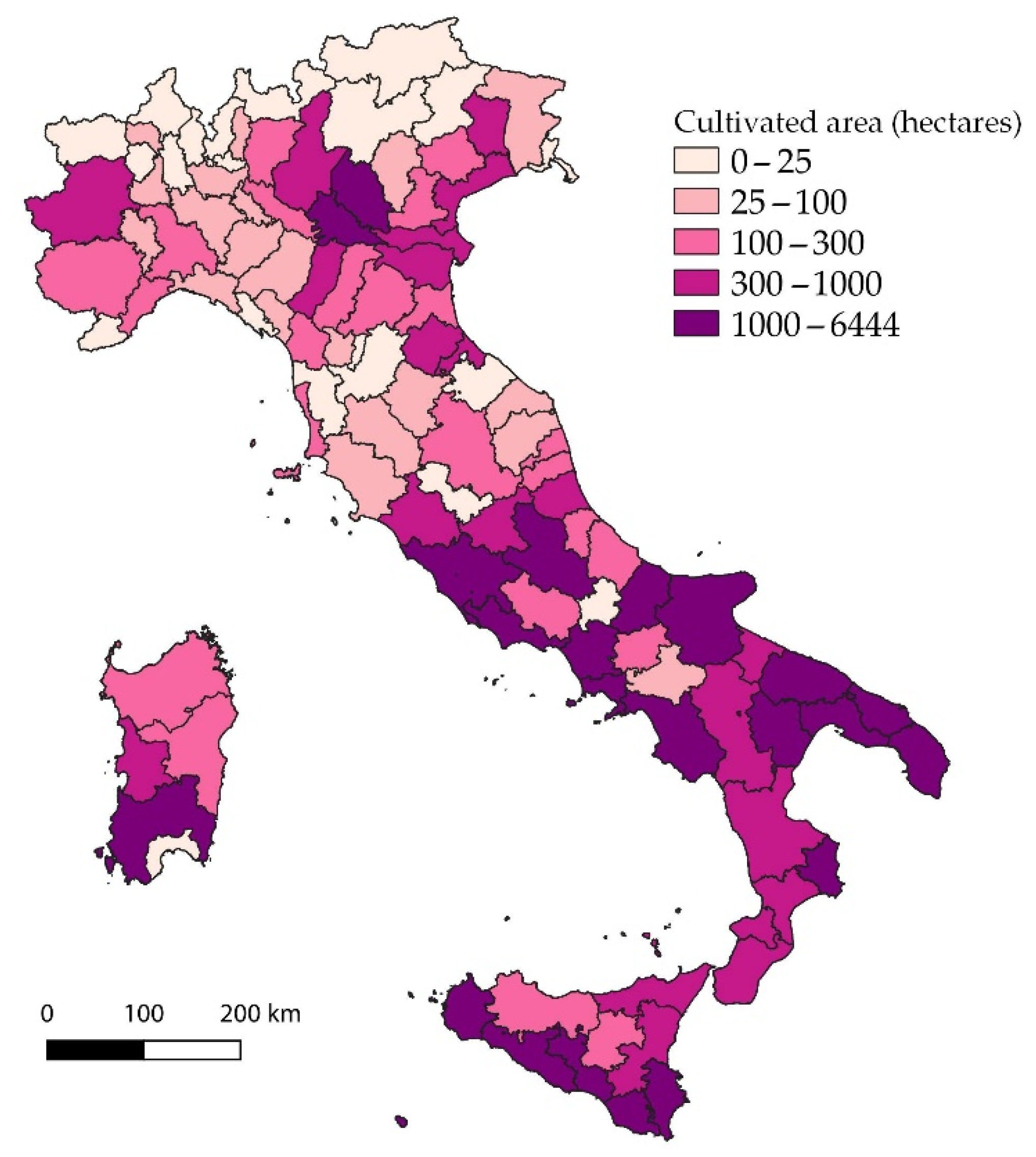
The first result concerns the calculation of the areas cultivated with the crops examined in Italy in the year of analysis [31]. In percentage terms, the most important crop that emerged from the ISTAT database was open-air fennel, which represented 28% of the total (Table 3).
Table 3.
The total area cultivated with crops, used as a study in this paper for each Italian province. Values represent the total hectares and the percentage of total crops reported in Table 1.
Therefore, based only on the chosen crops under examination, the APCoeff was calculated for each plastic product considered (Table 4) and added up to obtain the total (APCoeff_tot). This value indicates the kg of plastic used each year in each m2 of the crop. Since the value of the cultivated area is in hectares and the APCoeff is relative to m2, a conversion was necessary. The complete scheme of individual plastic structure data for each crop is shown in Appendix A (Table A1).
Table 4.
The different APCoeffs calculated for every single crop. Values are expressed in kg·m−2·years−1. Furthermore, each coefficient is expressed as a percentage of the total (APCoeff_tot). Where there are no values, it means that, for that crop, the respondents did not use that type of product. In Appendix A—Table A1.
From the APCoeff calculation, it emerges that the crops with the highest use of plastic recorded are melons and watermelons in the greenhouse, with 0.254 kg of plastic used for each square meter of cultivation every year. The crops with less plastic use are eggplants, bell peppers, and beans in open air, with a value of 0.008 kg·m−2·years−1, since the only plastic structures used were irrigation pipes. Obviously, greenhouse crops have higher values of the coefficient because most of the plastic material used refers to the greenhouse or tunnel cover (values around 92% for some crops and 60% for others). Moreover, by applying the coefficients implemented to the total areas cultivated with the crops under examination in a tabular way for the whole of Italy, it emerges that most of the tons produced every year are derived from the watermelon open air, with almost 40% of the total followed by the melons in greenhouses, with 13.35% (Table 5). Some, instead, have extremely low values.
Table 5.
Total tons per year of plastic produced in Italy for each type of crop examined. The values are also expressed as percentages of the totals.
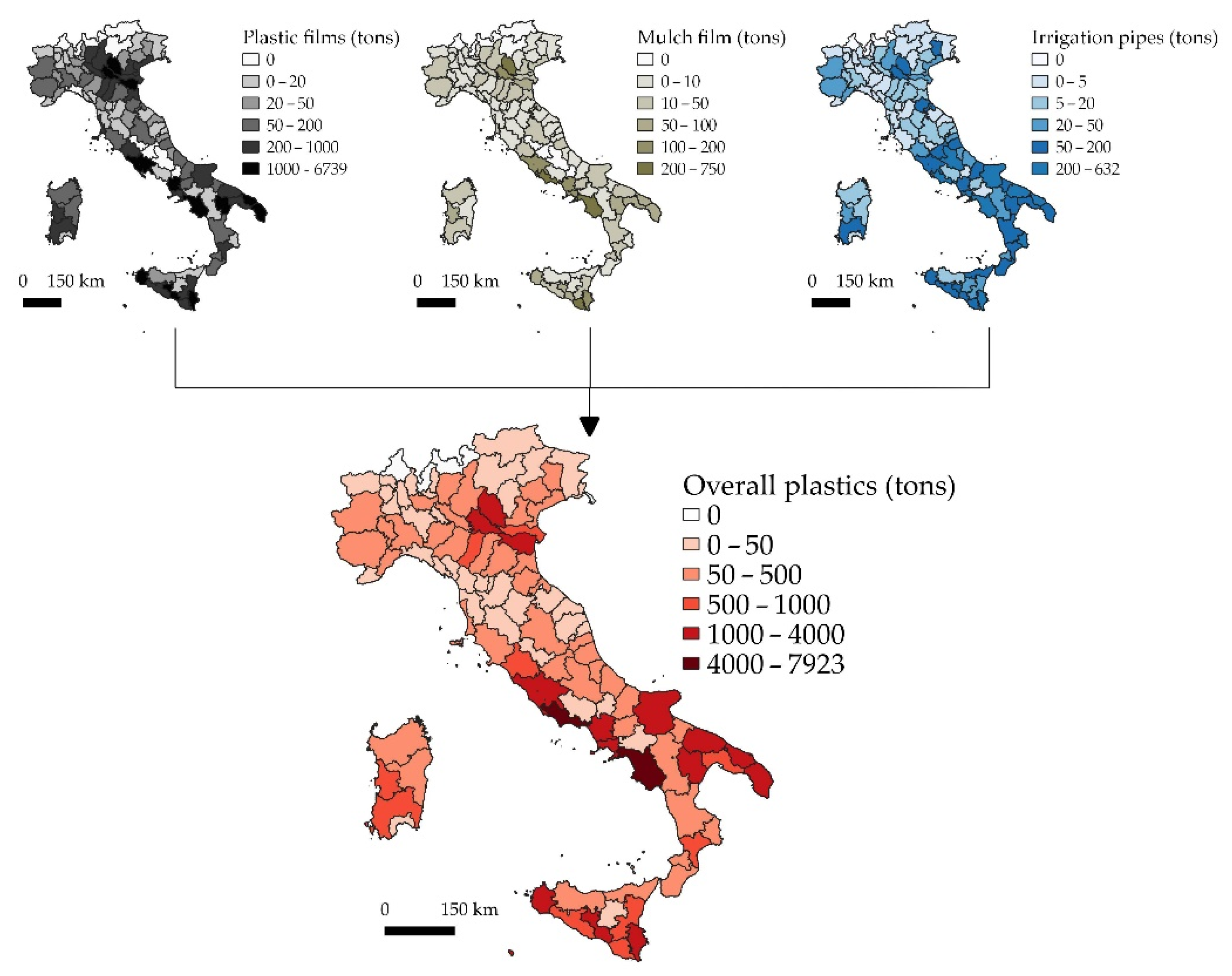
From the spatial join between the previously elaborated data and the administrative boundaries, it was possible to spatialize within the Italian provinces the quantities of the different types of plastics. Considering the size of the elaborated database, Figure 3 shows an example of mapping for one of the most cultivated crops among those considered in the study (as shown in Table 4) and for which the greatest amount of plastic is used (as shown in Table 5), i.e., watermelon in open air.
Figure 3.
Example of calculation of total tons of plastic used in a year in the case of watermelon cultivation in open air.
Thanks to the GIS environment, it is possible to perform these operations in iterative and consequential ways, with enormous gains in time and, above all, providing spatially explicit information that can be calibrated in relation to the starting database [36]. The realization of the database in the form of a spreadsheet is fundamental because it allows performing surveys and analyses at different levels without having to perform complicated operations and, therefore, it is not too difficult for those who do not have high knowledge about geospatial techniques. In this way, the methodology implemented can be easily replicated in an immediate manner in relation to the information to be obtained. Therefore, for all crops analyzed, the same method and technique of calculation of APW expressed in tons per year was applied. Spatialization by Italian provinces allowed us to map plastics for each of them, differentiating them by type, and then making the overall total of tons of plastic waste produced each year (Figure 4).
Figure 4.
Mapping of the plastics produced each year by the crops examined within the Italian provinces.
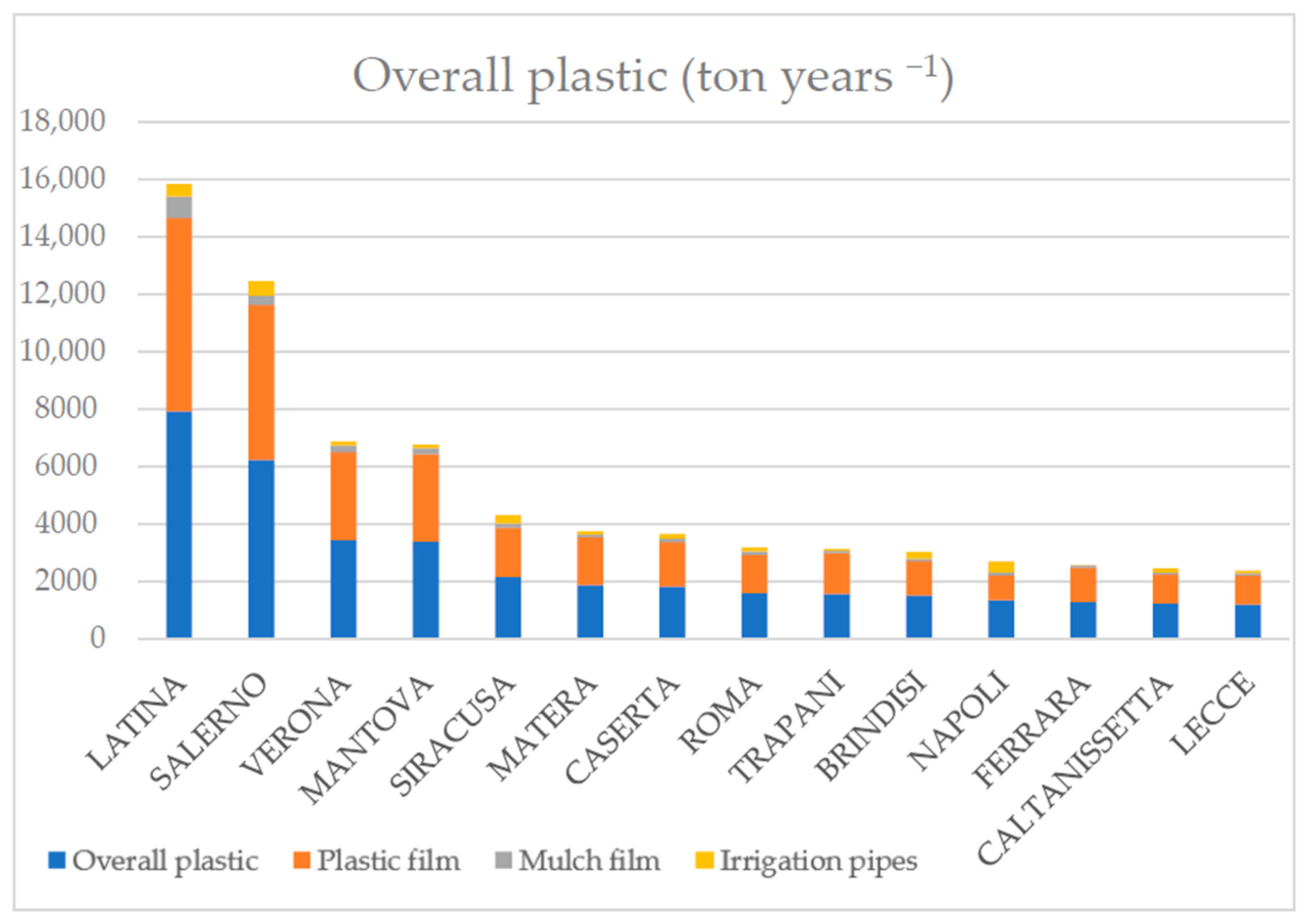
The result is composed of four maps connected to a numerical database in which the province that produces a greater amount of plastic types and the one that produces more can be evaluated. In this way, in addition to providing data, the methodology can be the basis for the development of a complex computerized system to identify centers for the disposal of APW [41]. Given the dimensions of the data produced (Table A2), provinces that produce more than 2% of the total annually were arbitrarily chosen to produce a summary graph (Figure 5). In addition, the complete tabular database can be found in Appendix A.
Figure 5.
Graph of the production of the different types of plastics considered for some of the provinces with the greatest amounts.
From the analysis, it is clear that the provinces of Latina and Salerno (Latium and Campania regions) have greater quantities of plastic in relation to the examined crops, and that in all cases, the plastic films have greater weight on the overall total. These data have already emerged from the information previously elaborated, but in this phase, they provided new information about the areas with the highest amounts of plastic, expanding the studies already present in the literature to the study areas of southern Italy [35,36].
The main objective of this work was to create an open source GIS-based methodology to preliminarily quantify the potential APW present in a given territorial and administrative area, in a way that easily implements with commonly available data and, at the same time, provides data that can be used in subsequent monitoring or decision-making phases [42] for the protection of soil from pollution by micro- and nanoplastics [43]. This study shows how the GIS approach is essential for the smarter and sustainable management of agricultural activities as it can put together data that are apparently difficult to spatialize [44].
Secondly, it provides basic data on the management of plastics in Italy, as it is one of the areas that uses the most plastic (Agricultural Plastic Europe, 2021). This kind of analysis, even if on a very large scale, since it is one of the NUT3 regions, provides useful indications to public decision makers to address specific strategies and actions to manage agricultural plastic waste and support agri-food supply chains [45,46].
Compared with a previous study carried out on the entire Italian territory, [30], it emerges that the data, although referring to different years and plastic products, are comparable and in the same order of magnitude. Indeed, the coefficient values found for most crops of about 0.15 kg m2 per year are almost the same, particularly for greenhouse plastic film. On the other hand, mulching films and irrigation pipes show slightly different values. This can be explained by the fact that, over the years, the technical characteristics (thicknesses in particular) of the plastic products used have changed. Moreover, compared to the total production (in tons per hectare per year) of agricultural plastics, they were noted by a little more than half, because in this study not all plastic products and crops grown in Italy were taken into account, which will be done in future research.
To set up a methodology that could be replicated in other European contexts [47], it was assumed that all of the same types of plastics were used throughout Italy, bearing in mind that the interviewees represented important samples of the major fruit and vegetable productions of Puglia and Basilicata Regions. In addition, not all types of crops that use plastics were considered as this is a preliminary study that focused more on the methodology than on a complete study of the situation of APW in Italy. However, since the methodology can be modulated in relation to the level of detail of the data available, the technical characteristics of the plastics can be modified in relation to the specific survey to be carried out. In fact, the proposed methodology can be adapted to the type of survey to be carried out since, once the GIS project is set up, changing the administrative area, the type of crops, the number of interviewees, and the agricultural census data, the analysis of the number of plastics produced can be made even more accurate and specific. This work presents some novelties with respect to what was proposed in other similar works since it allows calculating the quantity of agricultural plastic waste at a nationwide level in rapid and accurate ways. Furthermore, the integration and direct connection between spreadsheets and the GIS environment allows one to modulate and modify the starting data at will and in a simple way, even for one who is unfamiliar with spatial analyses. Another goal for the future is to put together the spatial analyses of statistical data and the classifications of satellite images presented in the two parts of the work to improve this methodology of the investigation [48]. Indeed, by integrating the remotely derived agricultural plastic surfaces (part I) and the agricultural plastic coefficients presented in this study (part II), it will be possible to make a more precise and spatially accurate estimate in order to implement an overall methodology that can allow an effective calculation of the distribution of plastics in the territory. In this way, a useful tool will be provided to support waste planning activities in agriculture to increase their environmental sustainability.
4. Conclusions
Plastics are widely used in agriculture, and they provide numerous services. In many cases, plastics have become the most economical solution to sustaining higher crop production. However, the use of plastics comes with challenges for the management of the resulting plastic waste and environmental contamination with plastic debris. Reducing the plastic footprint in agriculture requires the collaboration of farmers, plastic industries, researchers, and politicians to ensure the sustainable use of our resources and the protection of the environment.
However, the main step is to quantify the APS and spatialize it at the highest possible level of detail. Semi-automatic techniques for the classification of satellite images or aerial photos are certainly rapid and accurate tools for detecting large areas of land. However, this deductive approach must also be combined with the inductive approach, as it makes the actual classification and computation of APS much more precise and specific. For the integration of the two approaches, the point of connection is represented by the open source GIS environment, which guarantees easy implementation of the two methods—a standardization and modulation of procedures without excessive costs. Furthermore, the methodologies proposed in parts I and II guarantee usability outside the academic environment, as the techniques and data used are easily exploitable even without high technical skills.
Thus, the results achieved in this second study provide additional tools useful for the realization of a digital atlas that could be realized at the European scale, exploding the open-source GIS environment.
Author Contributions
The authors contributed to this paper. G.C. conceptualized and developed the research design, methodology, manuscript writing, data analysis, and elaboration, D.S. revised the manuscript, E.S. and G.V. revised and integrated the manuscript writing, and P.P. supervised the work. All authors have read and agreed to the published version of the manuscript.
Funding
This research was funded by the Project “Plastic in Agricultural Production: Impacts, Lifecycles and Long-term sustainability—PAPILLONS”, financed by the European Union—Topic: SFS-21-2020 emerging challenges for soil management—Sub-Topic B [2020]: emerging challenges for soil management: use of plastic in agriculture (RIA)—grant agreement ID: 101000210.
Institutional Review Board Statement
Not applicable.
Informed Consent Statement
Not applicable.
Data Availability Statement
The raw data are reported in the Appendix A. The elaborated data presented in this study are available upon request from the corresponding author. The funders had no role in the design of the study; in the collection, analyses, or interpretation of data; in the writing of the manuscript, or in the decision to publish the results.
Acknowledgments
The authors wish to thank Carlo Sivolella, who is part of the technical staff at SAFE, the University of Basilicata, for his kind technical support in retrieving the statistical data on crops cultivated in Italian provinces.
Conflicts of Interest
The authors declare no conflict of interest.
Appendix A
Table A1.
Technical characteristics of the plastics and calculations for crops of different APCoeffs.
Table A1.
Technical characteristics of the plastics and calculations for crops of different APCoeffs.
| Crops | Plastic Topology | Thickness 1 (μm) | Density 2 (kg·m−3 or kg·m−2) | Years (n.) | CACorr (adim.) | APCoeff (kg·m−2·years−1) |
|---|---|---|---|---|---|---|
| Canteen Cucumber in Greenhouse | Plastic films | 160 | 1250 | 2 | 1.5 | 0.150 |
| Mulch films | 20 | 1300 | 2 | 0.77 | 0.010 | |
| Irrigation pipes | 0.008 | 2 | 1.1 | 0.004 | ||
| Tot (APCoeff_tot) | 0.164 | |||||
| French Bean in Greenhouse | Plastic films | 160 | 1250 | 2 | 1.5 | 0.150 |
| Mulch films | 20 | 1300 | 2 | 0.77 | 0.010 | |
| Irrigation pipes | 0.008 | 2 | 1.1 | 0.004 | ||
| Tot (APCoeff_tot) | 0.164 | |||||
| Lettuce in Greenhouse | Plastic films | 160 | 1250 | 2 | 1.5 | 0.150 |
| Mulch films | 20 | 1300 | 2 | 0.77 | 0.010 | |
| Irrigation pipes | 0.008 | 2 | 1.1 | 0.004 | ||
| Tot (APCoeff_tot) | 0.164 | |||||
| Melon in Greenhouse | Plastic films (Greenhouse) | 160 | 1250 | 2 | 1.5 | 0.150 |
| Plastic films (Tunnel) | 120 | 1250 | 0.5 | 0.31 | 0.093 | |
| Mulch films | 20 | 1300 | 1 | 0.3 | 0.008 | |
| Irrigation pipes | 0.008 | 1 | 0.4 | 0.003 | ||
| Tot (APCoeff_tot) | 0.254 | |||||
| Watermelon in Greenhouse | Plastic films (Greenhouse) | 160 | 1250 | 2 | 1.5 | 0.150 |
| Plastic films (Tunnel) | 120 | 1250 | 0.5 | 0.31 | 0.093 | |
| Mulch films | 20 | 1300 | 1 | 0.3 | 0.008 | |
| Irrigation pipes | 0.008 | 1 | 0.4 | 0.003 | ||
| Tot (APCoeff_tot) | 0.254 | |||||
| Fennel in Greenhouse | Plastic films | 160 | 1250 | 2 | 1.5 | 0.150 |
| Mulch films | 20 | 1300 | 2 | 0.77 | 0.010 | |
| Irrigation pipes | 0.008 | 2 | 1.1 | 0.004 | ||
| Tot (APCoeff_tot) | 0.164 | |||||
| Strawberry in Greenhouse | Plastic films | 160 | 1250 | 2 | 1.5 | 0.150 |
| Mulch films | 20 | 1300 | 2 | 0.77 | 0.010 | |
| Irrigation pipes | 0.008 | 2 | 1.1 | 0.004 | ||
| Tot (APCoeff_tot) | 0.164 | |||||
| Pea in Open Air | Plastic films | |||||
| Mulch films | 10 | 2600 | 1 | 1 | 0.026 | |
| Irrigation pipes | 0.008 | 1 | 1 | 0.008 | ||
| Tot (APCoeff_tot) | 0.034 | |||||
| Asparagus in Open Air | Plastic films | |||||
| Mulch films | ||||||
| Irrigation pipes | 0.008 | 1 | 1.66 | 0.013 | ||
| Tot (APCoeff_tot) | 0.013 | |||||
| Radicchio in Open Air | Plastic films | |||||
| Mulch films | ||||||
| Irrigation pipes | 0.008 | 1 | 2 | 0.016 | ||
| Tot (APCoeff_tot) | 0.016 | |||||
| Celery in Open Air | Plastic films | |||||
| Mulch films | ||||||
| Irrigation pipes | 0.008 | 1 | 2 | 0.016 | ||
| Tot (APCoeff_tot) | 0.016 | |||||
| Eggplant in Open Air | Plastic films | |||||
| Mulch films | ||||||
| Irrigation pipes | 0.008 | 1 | 1 | 0.008 | ||
| Tot (APCoeff_tot) | 0.008 | |||||
| Bell Pepper in Open Air | Plastic films | |||||
| Mulch films | ||||||
| Irrigation pipes | 0.008 | 1 | 1 | 0.008 | ||
| Tot (APCoeff_tot) | 0.008 | |||||
| Bean and Kidney Bean in Open Air | Plastic films | |||||
| Mulch films | ||||||
| Irrigation pipes | 0.008 | 1 | 1 | 0.008 | ||
| Tot (APCoeff_tot) | 0.008 | |||||
| Lettuce in Open Air | Plastic films | |||||
| Mulch films | ||||||
| Irrigation pipes | 0.008 | 1 | 2 | 0.016 | ||
| Tot (APCoeff_tot) | 0.016 | |||||
| Zucchini in Open Air | Plastic films | |||||
| Mulch films | 20 | 1300 | 1 | 0.9 | 0.023 | |
| Irrigation pipes | 0.008 | 1 | 1 | 0.008 | ||
| Tot (APCoeff_tot) | 0.031 | |||||
| Swiss Chard in Open Air | Plastic films | |||||
| Mulch films | ||||||
| Irrigation pipes | 0.008 | 1 | 2 | 0.016 | ||
| Tot (APCoeff_tot) | 0.016 | |||||
| Watermelon in Open Air | Plastic films | 120 | 1500 | 0.5 | 0.5 | 0.180 |
| Mulch films | 20 | 1300 | 1 | 0.5 | 0.013 | |
| Irrigation pipes | 0.008 | 1 | 0.33 | 0.003 | ||
| Tot (APCoeff_tot) | 0.196 | |||||
| Fennel in Open Air | Plastic films | |||||
| Mulch films | ||||||
| Irrigation pipes | 0.008 | 1 | 2 | 0.016 | ||
| Tot (APCoeff_tot) | 0.016 | |||||
| Endive (Curly and Escarole) in Open Air | Plastic films | |||||
| Mulch films | ||||||
| Irrigation pipes | 0.008 | 1 | 2 | 0.016 | ||
| Tot (APCoeff_tot) | 0.016 |
1 For the calculation of the APCoeff, the value was converted to meters. 2 As stated in the article, kg·m2 refer to irrigation pipes only.
Table A2.
Amount of tons per year produced in total for all crops examined. Values are also expressed as a percentage of the total.
Table A2.
Amount of tons per year produced in total for all crops examined. Values are also expressed as a percentage of the total.
| Provinces | Tons years−1 | % | Provinces | Tons years−1 | % | Provinces | Tons years−1 | % | Provinces | Tons years−1 | % | Provinces | Tons years−1 | % |
|---|---|---|---|---|---|---|---|---|---|---|---|---|---|---|
| AGRIGENTO | 745.52 | 1.37 | CASERTA | 1824.67 | 3.34 | LATINA | 7923.03 | 14.52 | PERUGIA | 195.13 | 0.36 | SUD SARD. | 664.22 | 1.22 |
| ALESSANDRIA | 107.91 | 0.20 | CATANIA | 707.32 | 1.30 | LECCE | 1189.04 | 2.18 | PESARO E URB. | 16.82 | 0.03 | TARANTO | 950.56 | 1.74 |
| ANCONA | 35.65 | 0.07 | CATANZARO | 569.46 | 1.04 | LECCO | 28.87 | 0.05 | PESCARA | 70.86 | 0.13 | TERAMO | 334.32 | 0.61 |
| AOSTA | 0.93 | 0.00 | CHIETI | 116.91 | 0.21 | LIVORNO | 243.07 | 0.45 | PIACENZA | 174.4 | 0.32 | TERNI | 1.44 | 0.00 |
| AREZZO | 30.04 | 0.06 | COMO | 0 | 0.00 | LODI | 42.86 | 0.08 | PISA | 3.91 | 0.01 | TORINO | 154.53 | 0.28 |
| AS.PICENO | 57.99 | 0.11 | COSENZA | 255.96 | 0.47 | LUCCA | 45.76 | 0.08 | PISTOIA | 23.35 | 0.04 | TRAPANI | 1561.92 | 2.86 |
| ASTI | 52.6 | 0.10 | CREMONA | 361.38 | 0.66 | MACERATA | 10.28 | 0.02 | PORDENONE | 109.06 | 0.20 | TRENTO | 0.8 | 0.00 |
| AVELLINO | 10.99 | 0.02 | CROTONE | 378.53 | 0.69 | MANTOVA | 3381.94 | 6.20 | POTENZA | 51.74 | 0.09 | TREVISO | 66.89 | 0.12 |
| BARI | 1068.27 | 1.96 | CUNEO | 181.93 | 0.33 | M. CARRARA | 23.53 | 0.04 | PRATO | 1.28 | 0.00 | TRIESTE | 0 | 0.00 |
| BAT | 182.37 | 0.33 | ENNA | 23.55 | 0.04 | MATERA | 1875.56 | 3.44 | RAGUSA | 918.19 | 1.68 | UDINE | 14.01 | 0.03 |
| BELLUNO | 0.49 | 0.00 | FERMO | 29.13 | 0.05 | MESSINA | 52.01 | 0.10 | RAVENNA | 223.52 | 0.41 | VARESE | 1.9 | 0.00 |
| BENEVENTO | 197.33 | 0.36 | FERRARA | 1281.47 | 2.35 | MILANO | 59.53 | 0.11 | REGGIO CAL- | 147.64 | 0.27 | VENEZIA | 496.55 | 0.91 |
| BERGAMO | 357.94 | 0.66 | FIRENZE | 22.42 | 0.04 | MODENA | 445.95 | 0.82 | REGGIO EMILIA | 512.04 | 0.94 | VS | 0 | 0.00 |
| BIELLA | 1.98 | 0.00 | FOGGIA | 1025.59 | 1.88 | MONZA | 8.7 | 0.02 | RIETI | 53.28 | 0.10 | VERCELLI | 24.12 | 0.04 |
| BOLOGNA | 239.05 | 0.44 | FORL. CES. | 215.49 | 0.39 | NAPOLI | 1344.75 | 2.46 | RIMINI | 151.87 | 0.28 | VERONA | 3437.85 | 6.30 |
| BOLZANO | 2.72 | 0.00 | FROSINONE | 36.01 | 0.07 | NOVARA | 10.74 | 0.02 | ROMA | 1591.06 | 2.92 | VIBO VAL. | 191.31 | 0.35 |
| BRESCIA | 485.75 | 0.89 | GENOVA | 4.63 | 0.01 | NUORO | 114.45 | 0.21 | ROVIGO | 765.39 | 1.40 | VICENZA | 38.85 | 0.07 |
| BRINDISI | 1513.65 | 2.77 | GORIZIA | 14.04 | 0.03 | ORISTANO | 991.11 | 1.82 | SALERNO | 6234.53 | 11.42 | VITERBO | 576.42 | 1.06 |
| CAGLIARI | 10.86 | 0.02 | GROSSETO | 128.76 | 0.24 | PADOVA | 324.75 | 0.60 | SASSARI | 219.55 | 0.40 | 54,569.23 | 100 | |
| CALTANISSETTA | 1225.41 | 2.25 | IMPERIA | 4.47 | 0.01 | PALERMO | 58.53 | 0.11 | SAVONA | 59.67 | 0.11 | |||
| CAMPOBASSO | 235.06 | 0.43 | ISERNIA | 2.72 | 0.00 | PARMA | 56.24 | 0.10 | SIENA | 12.79 | 0.02 | |||
| LA SPEZIA | 11.25 | 0.02 | PAVIA | 27.8 | 0.05 | SIRACUSA | 2153.56 | 3.95 | ||||||
| L’AQUILA | 347.2 | 0.64 | SONDRIO | 0 | 0.00 |
References
- European Commission. EU Soil Strategy for 2030, COM (2021) 699 Final. Available online: https://ec.europa.eu/environment/publications/eu-soil-strategy-2030_en (accessed on 21 March 2022).
- Bouma, J.; Montanarella, L.; Evanylo, G. The challenge for the soil science community to contribute to the implementation of the UN Sustainable Development Goals. Soil Use Manag. 2019, 35, 538–546. [Google Scholar] [CrossRef]
- European Commission. A Soil Deal for Europe: Implementation Plan. Available online: https://ec.europa.eu/info/sites/default/files/research_and_innovation/funding/documents/soil_mission_implementation_plan_final_for_publication.pdf (accessed on 1 April 2022).
- FAO. Assessment of Agricultural Plastics and Their Sustainability—A Call for Action; FAO: Rome, Italy, 2021. [Google Scholar] [CrossRef]
- Zhang, D.; Ng, E.L.; Hu, W.; Wang, H.; Galaviz, P.; Yang, H.; Sun, W.; Li, C.; Ma, X.; Fu, B.; et al. Plastic pollution in croplands threatens long-term food security. Glob. Chang. Biol. 2020, 26, 3356–3367. [Google Scholar] [CrossRef] [PubMed]
- Leslie, H.A.; van Velzen, M.J.M.; Brandsma, S.H.; Dick Vethaak, A.; Garcia-Vallejo, J.J.; Lamoree, M.H. Discovery and quantification of plastic particle pollution in human blood. Environ. Int. 2022, 163, 107199. [Google Scholar] [CrossRef]
- EIP-AGRI Focus Group: Reducing the Plastic Footprint of Agriculture. Available online: https://ec.europa.eu/eip/agriculture/sites/default/files/eip-agri_fg_plastic_footprint_final_report_2021_en.pdf (accessed on 21 March 2022).
- Plastics Europe. Plastics—The Facts 2018. Available online: https://plasticseurope.org/wp-content/uploads/2021/10/2018-Plastics-the-facts.pdf (accessed on 30 March 2022).
- Alimi, O.S.; Farner Budarz, J.; Hernandez, L.M.; Tufenkji, N. Microplastics and nanoplastics in aquatic environments: Aggregation, deposition, and enhanced contaminant transport. Environ. Sci. Technol. 2018, 52, 1704–1724. [Google Scholar] [CrossRef] [PubMed]
- Dissanayake, P.V.; Kim, S.; Sarkar, B.; Oleszczuk, P.; Sang, M.K.; Haque, M.N.; Ahn, J.H.; Bank, M.S.; Ok, Y.S. Effects of microplastics on the terrestrial environment: A critical review. Environ. Res. 2022, 209, 112734. [Google Scholar] [CrossRef]
- Boots, B.; Russell, C.W.; Green, D.S. Effects of microplastics in soil ecosystems: Above and below ground. Environ. Sci. Technol. 2019, 53, 11496–11506. [Google Scholar] [CrossRef]
- Scarascia-Mugnozza, G.; Sica, C.; Russo, G. Plastic Materials in European Agriculture: Actual Use and Perspectives. J. Agric. Eng. 2012, 42, 15–28. [Google Scholar] [CrossRef]
- Picuno, C.; Godosi, Z.; Kuchta, K.; Picuno, P. Agrochemical plastic packaging waste decontamination for recycling: Pilot tests in Italy. J. Agric. Eng. 2019, 50, 99–104. [Google Scholar] [CrossRef]
- Picuno, P. Innovative Material and Improved Technical Design for a Sustainable Exploitation of Agricultural Plastic Film. Polym. Technol. Eng. 2014, 53, 1000–1011. [Google Scholar] [CrossRef]
- Espí, E.; Salmerón, A.; Fontecha, A.; García, Y.; Real, A.I. Plastic films for agricultural applications. J. Plast. Film. Sheeting 2006, 22, 85–102. [Google Scholar] [CrossRef]
- Pazienza, P.; De Lucia, C. For a new plastics economy in agriculture: Policy reflections on the EU strategy from a local perspective. J. Clean. Prod. 2020, 253, 119844. [Google Scholar] [CrossRef]
- Astner, A.F.; Hayes, D.G.; O’Neill, H.; Evans, B.R.; Pingali, S.V.; Urban, V.S.; Young, T.M. Formazione meccanica di materiali micro e nano-plastici per studi ambientali in ecosistemi agricoli. Sci. Total Environ. 2019, 685, 1097–1106. [Google Scholar] [CrossRef] [PubMed]
- Piehl, S.; Leibner, A.; Löder, M.G.J.; Dris, R.; Bogner, C.; Laforsch, C. Identification and quantification of macro- and microplastics on an agricultural farmland. Sci. Rep. 2018, 8, 17950. [Google Scholar] [CrossRef] [Green Version]
- Fakour, H.; Lo, S.-L.; Yoashi, N.T.; Massao, A.M.; Lema, N.N.; Mkhontfo, F.B.; Jomalema, P.C.; Jumanne, N.S.; Mbuya, B.H.; Mtweve, J.T.; et al. Quantification and Analysis of Microplastics in Farmland Soils: Characterization, Sources, and Pathways. Agriculture 2021, 11, 330. [Google Scholar] [CrossRef]
- European Union—Action to Tackle the Issue of Plastic Waste. Available online: https://www.eca.europa.eu/Lists/ECADocuments/RW20_04/RW_Plastic_waste_EN.pdf (accessed on 1 April 2022).
- Duque-Acevedo, M.; Belmonte-Ureña, L.J.; Cortés-García, F.J.; Camacho-Ferre, F. Agricultural waste: Review of the evolution, approaches and perspectives on alternative uses. Glob. Ecol. Conserv. 2020, 22, e00902. [Google Scholar] [CrossRef]
- Scarascia-Mugnozza, G.; Sica, C.; Picuno, P. The Optimization of the Management of Agricultural Plastic Waste in Italy Using a Geographical Information System. Acta Hortic. 2008, 801, 219–226. [Google Scholar] [CrossRef]
- Vox, G.; Loisi, R.V.; Blanco, I.; Mugnozza, G.S.; Schettini, E. Mapping of agriculture plastic waste. Agric. Agric. Sci. Procedia 2016, 8, 583–591. [Google Scholar] [CrossRef] [Green Version]
- Nanna, M.; Batista, M.T.; Baptista, F.J.; Schettini, E.; Vox, G. Mapping greenhouse plastic wastes in the west region of Portugal. Acta Hortic. 2018, 1227, 257–264. [Google Scholar] [CrossRef]
- Cillis, G.; Statuto, D.; Schettini, E.; Vox, G.; Picuno, P. Implementing a GIS-Based Digital Atlas of Agricultural Plastics to Reduce Their Environmental Footprint; Part I: A Deductive Approach. Appl. Sci. 2022, 12, 1330. [Google Scholar] [CrossRef]
- Yang, D.; Chen, J.; Zhou, Y.; Chen, X.; Chen, X.; Cao, X. Mapping plastic greenhouse with medium spatial resolution satellite data: Development of a new spectral index. ISPRS J. Photogramm. Remote Sens. 2017, 128, 47–60. [Google Scholar] [CrossRef]
- Scarascia Mugnozza, G.; Schettini, E.; Loisi, R.V.; Blanco, I.; Vox, G. Georeferencing of agricultural plastic waste. Riv. Studi Sulla Sostenibilità 2016, 1, 71–82. [Google Scholar] [CrossRef]
- Cillis, G.; Statuto, D.; Picuno, P. Historical GIS as a Tool for Monitoring, Preserving and Planning Forest Landscape: A Case Study in a Mediterranean Region. Land 2021, 10, 851. [Google Scholar] [CrossRef]
- Cillis, G.; Statuto, D.; Picuno, P. Integrating Remote-Sensed and Historical Geodata to Assess Interactions Between Rural Buildings and Agroforestry Land. J. Environ. Eng. Landsc. Manag. 2021, 29, 229–243. [Google Scholar] [CrossRef]
- Briassoulis, D.; Babou, E.; Hiskakis, M.; Scarascia-Mugnozza, G.; Picuno, P.; Guarde, D.; Dejean, C. Review, mapping and analysis of the agricultural plastic waste generation and consolidation in Europe. Waste Manag. Res. J. Sustain. Circ. Econ. 2013, 31, 1262–1278. [Google Scholar] [CrossRef] [PubMed]
- ISTAT. Censimenti Dell’agricoltura. Available online: https://www.istat.it/it/censimenti-permanenti/censimenti-precedenti/agricoltura (accessed on 30 January 2022).
- Eurostat. Agricultural Database. Available online: https://ec.europa.eu/eurostat/web/agriculture/data/database (accessed on 5 April 2022).
- ISMEA Reports. Available online: https://www.ismea.it/flex/cm/pages/ServeBLOB.php/L/IT/IDPagina/9886 (accessed on 20 April 2022).
- Pardossi, A.; Tognoni, F. Greenhouse industry in Italy. Acta Hortic. 1999, 481, 769–770. [Google Scholar] [CrossRef]
- Blanco, I.; Loisi, R.V.; Sica, C.; Schettini, E.; Vox, G. Agricultural plastic waste mapping using GIS. A case study in Italy. Resour. Conserv. Recycl. 2018, 137, 229–242. [Google Scholar] [CrossRef]
- Parlato, M.C.; Valenti, F.; Porto, S.M. Covering plastic films in greenhouses system: A GIS-based model to improve post use suistainable management. J. Environ. Manag. 2020, 263, 110389. [Google Scholar] [CrossRef]
- STAT Database. Available online: http://dati.istat.it/ (accessed on 30 April 2022).
- Mihai, F.C.; Gündoğdu, S.; Markley, L.A.; Olivelli, A.; Khan, F.R.; Gwinnett, C.; Gutberlet, J.; Reyna-Bensusan, N.; Llanquileo-Melgarejo, P.; Meidiana, C.; et al. Plastic Pollution, Waste Management Issues, and Circular Economy Opportunities in Rural Communities. Sustainability 2022, 14, 20. [Google Scholar] [CrossRef]
- Ibrahim, E.; Gobin, A. Sentinel-2 Recognition of Uncovered and Plastic Covered Agricultural Soil. Remote. Sens. 2021, 13, 4195. [Google Scholar] [CrossRef]
- Waste Management Planning. Available online: https://ec.europa.eu/environment/waste/plans/index.htm (accessed on 19 October 2021).
- Morsink-Georgali, P.Z.; Afxentiou, N.; Kylili, A.; Fokaides, P.A. Definition of optimal agricultural plastic waste collection centers with advanced spatial analysis tools. Clean. Eng. Technol. 2021, 5, 100326. [Google Scholar] [CrossRef]
- Agriculture Plastic Europe. Statistics 2021. Available online: https://apeeurope.eu/statistics/ (accessed on 5 March 2022).
- Debeljak, M.; Trajanov, A.; Kuzmanovski, V.; Schröder, J.; Sandén, T.; Spiegel, H.; Wall, D.P.; Van de Broek, M.; Rutgers, M.; Bampa, F.; et al. A Field-Scale Decision Support System for Assessment and Management of Soil Functions. Front. Environ. Sci. 2019, 7, 115. [Google Scholar] [CrossRef] [Green Version]
- Zhai, Z.; Martínez, J.F.; Beltran, V.; Martínez, N.L. Decision Support Systems for Agriculture 4.0: Survey and Challenges. Comput. Electron. Agric. 2020, 170, 105256. [Google Scholar] [CrossRef]
- Carletto, C.; Jolliffe, D.; Banerjee, R. From Tragedy to Renaissance: Improving Agricultural Data for Better Policies. J. Dev. Stud. 2015, 51, 133–148. [Google Scholar] [CrossRef]
- Notarnicola, B.; Tassielli, G.; Renzulli, P.A.; Di Capua, R.; Saija, G.; Salomone, R.; Primerano, P.; Petti, L.; Raggi, A.; Casolani, N.; et al. Life cycle inventory data for the Italian agri-food sector: Background, sources and methodological aspects. Int. J. Life Cycle Assess 2022. [Google Scholar] [CrossRef]
- PAPILLONS Project—Plastic in Agricultural Production: Impacts, Lifecycles and Long-Term Sustainability. Available online: https://www.papillons-h2020.eu/ (accessed on 20 March 2022).
- Lanorte, A.; De Santis, F.; Nolè, G.; Blanco, I.; Loisi, R.V.; Schettini, E.; Vox, G. Agricultural plastic waste spatial estimation by Landsat 8 satellite images. Comput. Electron. Agric. 2017, 141, 35–45. [Google Scholar] [CrossRef]
Publisher’s Note: MDPI stays neutral with regard to jurisdictional claims in published maps and institutional affiliations. |
© 2022 by the authors. Licensee MDPI, Basel, Switzerland. This article is an open access article distributed under the terms and conditions of the Creative Commons Attribution (CC BY) license (https://creativecommons.org/licenses/by/4.0/).