Data Management and Processing in Seismology: An Application of Big Data Analysis for the Doublet Earthquake of 2021, 03 March, Elassona, Central Greece

Abstract

On 3 March 2021 (10:16, UTC), a strong earthquake, M_w 6.3, occurred in Elassona, Central Greece. The epicenter was reported 10 km west of Tyrnavos. Another major earthquake followed this event on the same day at M_w 5.8 (3 March 2021, 11:45, UTC). The next day, 4 March 2021 (18:38, UTC), there was a second event with a similar magnitude as the first, M_w 6.2. Both events were 8.5 km apart. The following analysis shows that the previous events and the most significant aftershocks were superficial. However, historical and modern seismicity has been sparse in this area. Spatially, the region represents a transitional zone between different tectonic domains; the right-lateral slip along the western end of the North Anatolian Fault Zone (NAFZ) in the north Aegean Sea plate-boundary structure ends, and crustal extension prevails in mainland Greece. These earthquakes were followed by rich seismic activity recorded by peripheral seismographs and accelerometers. The installation of a dense, portable network from the Aristotle University of Thessaloniki team also helped this effort, installed three days after the seismic excitation, as seismological stations did not azimuthally enclose the area. In the present work, a detailed analysis was performed using seismological data. A seismological catalogue of 3.787 events was used, which was processed with modern methods to calculate 34 focal mechanisms (M_w > 4.0) and to recalculate the parameters of the largest earthquakes that occurred in the first two days.

1. Introduction

In-depth analyses of substantial seismological data from Central Greece are presented in this article. This extensive period of study using the latest state-of-the-art tools has never been performed before. With this analysis, we wanted to identify the faults responsible for this seismic excitation. Due to their dominance over the local seismic hazard, the faults triggered by the two main shocks must be resolved.

Whether these ruptures represent (one of) the seismic faults that generated the biggest shocks is currently debated. The hypocentral depths with the moderate-to-shallow dip angle in the InSAR images (Lekkas et al., 2021) suggest that the rupture of the primary seismic fault(s) emerged further to the south in the alpine zone, even though their direction fits the proposed nodal planes of the moment tensor solutions and the borehole findings. This study’s main task was to analyze a large volume of mainly seismological data to visualize the spatiotemporal distribution of the aftershock sequence.

Regarding the tectonic setting, Thessaly is located at the western end of the North Anatolian Fault Zone (NAFZ) in the north Aegean Sea, where the right-lateral slip along this plate-boundary structure ends and crustal extension prevails in mainland Greece [1,2]. The most prominent structural and geomorphic features strike NW-SE, such as the coastal and interior mountain ranges, bounding faults, and the late Tertiary sedimentary basins [3]. The seismicity of the Thessaly Basin is detected mainly along two fault zones relative to the maximum magnitude an earthquake can provide. The first is the northern fault zone, associated with earthquakes with magnitudes up to 6.5, and the second is the southern fault zone, related to earthquakes with a magnitude of 7.0.

In early March 2021, a doublet earthquake (M_w 6.3 and 6.2) occurred in the northern Thessalian region. The spatial distance of the two earthquakes was determined at only 8.5 km, while their time difference at 32 h. The first earthquake, magnitude 6.3, occurred on 3 March 2021 (10:16:08.3, UTC). The epicenter, as calculated and presented in the next paragraph, was found at φ = 39.7453° Ν, λ = 22.2340° Ε at a depth of 12 km. The earthquake was felt in Larissa, Trikala, and Kozani. This fact is due to the epicenter being a short distance from large cities. The epicenter was calculated 19 km northwest of the town of Larissa, 46 km northwest of the city of Trikala, and 72 km south of Kozani. According to the above, the mainshock caused extensive damage due to its short distance in a populated urban area, according to the European Mediterranean Seismological Center [4]; https://www.emsc-csem.org/#2 (accessed on 8 June 2022). Several buildings collapsed after this earthquake. One person died from the earthquake in the worst-hit village of Mesohori, near Elassona, where the local church and some old houses were severely damaged. Of the 3.675 homes, 1575 were deemed uninhabitable in the earthquake-stricken areas of Larissa, Elassona, Tyrnavos, and Farkadona. The earthquake caused much damage in the surrounding regions, and the Damasi primary school, built in 1938, suffered significant damage, resulting in its demolition eight days after the earthquake [5].

The second major earthquake occurred one day later, on 4 March 2021 (18:38:19.1, UTC), with M_w 6.2. The epicenter of this event was calculated at 39.7916° N, 22.1274° E, and at a depth of 8 km. Eight days later (12 March 2021, 12:57:50.6, UTC), a significant event, the third chronologically, eight days after the main one, with a magnitude M_w = 5.6, occurred in a different hypocentral area than the other two. A rich aftershock sequence followed these earthquakes, most felt by the area’s residents mainly due to their small focal depth. It is noted that in the first 24 h only, 381 events occurred, ranging from Μ_L 1.2 to 5.2. The intense aftershock sequence activity with M_L > 4.0 aftershocks continued for a few days, with a smaller magnitude but high aftershock occurrence rate. These two significant earthquakes have been the strongest in the region since 1941 when an earthquake of the magnitude M_L 6.3 occurred very close to the city of Larissa. The area of Thessaly, Central Greece, has been well known for its land subsidence phenomena since the 1980s [6,7,8,9,10,11].

Several institutions providing seismic moment tensors consistently determined an almost normal fault on the east–south and northwest plane for the first and second mainshocks. Moving in the fault, the two earthquakes had a similar focal mechanism. This means that they probably came from the same fault but different parts. From these data, we probably have the phenomenon of a seismic pair, which is extremely rare. Earthquake doublets commonly occur in subduction zones and are mainly characterized by having similar mechanisms, spatially and temporally [12,13,14], correlated with several tens of kilometers and hours to days, respectively [15,16]. They can mainly be explained by Coulomb stress triggering [17]. Intraplate earthquake doublets are rare and less studied.

Doublet earthquakes—and, more generally, multiple earthquakes—were initially identified as numerous earthquakes with nearly identical waveforms originating from the exact location [18]. They are now characterized as single earthquakes having two (or more) mainshocks of similar magnitude, sometimes occurring within tens of seconds but sometimes separated by years [19]. The magnitude similarity—often within four-tenths of a unit of magnitude—distinguishes multiple events from aftershocks [20], which start at approximately 1.2 magnitudes more minor than the parent shock [21,22] and decrease in magnitude and frequency according to known laws. Doublet events also have nearly identical seismic waveforms, as they come from the same rupture zone and stress field, whereas aftershocks, peripheral to the main rupture, typically reflect more diverse circumstances of origin [18]. Multiple events overlap in their focal areas (i.e., rupture zones), up to 100 km across for magnitude 7.5 earthquakes [23,24,25]. Doublets have been distinguished from triggered earthquakes, where the seismic waves’ energy triggers a distant earthquake with a different rupture zone, although it has been suggested that such a distinction reflects “imprecise taxonomy” more than any physical reality.

Figure 1 represents a general structure map showing the prefectures of the broader region of Central Greece. For the study area, the portable seismological station sites’ selection criterion was based on the existence and operation of permanent seismological and geodetic stations that were already installed. In addition, faults were collected from the international literature and digitized in QGIS.

The contribution of the present study is the localization of the significant events, i.e., epicenter (i.e., latitude and longitude), depth (d), and local magnitude (ML), as well as the calculation of the source parameters (i.e., strike, dip, rake, depth, and moment magnitude) for the strong events and all of the significant aftershocks using moment tensor inversion.

2. Data Description

Seismological broadband data were used to calculate the epicenter, the magnitude, and the focal depth for the mainshock and the second significant event and all events with a magnitude M_L > 5.0, in addition to the source parameters of both main earthquakes and their significant aftershocks. The data were collected, analyzed, and processed appropriately, studied in the next section in more detail [26,27].

Seismological Data

We used waveform data from three regional component stations of the Hellenic Unified Seismological Network (HUSN); detailed information is presented in

Table 1. Characteristics of the seismological stations in the broader area of Greece, the data from which were used in this study. Station coordinates are in decimal degrees; the elevation is in m. HL denotes the seismological network of the National Observatory of Athens; HT represents the seismological network of the University of Thessaloniki; MN designates the stations that belong to the MedNet (Mediterranean Seismological Network). Sources: Available online: https://bbnet.gein.noa.gr/HL (accessed on 15 March 2022); Available online: http://geophysics.geo.auth.gr (accessed on 15 March 2022) [28,29].

Stations	Latitude (°)	Longitude (°)	Code	Elevation (m)	Datalogger	Seismometer
THL	39.5646	22.0144	HL/MN	86	DR24-SC	STS-2
KZN	40.3033	21.7820	HL	791	DR24-SC	STS-2
NEO	39.3056	23.2218	HL	510	DR24-SC	KS2000M
JAN	39.6561	20.8487	HL	526	DR24-SC	CMG-3ESPC/60
EVR	38.9165	21.8105	HL	1037	DR24-SC	CMG-3ESPC/60
LIT	40.1003	22.4893	HT	568	Trident-B	CMG-3ESP/100
NEO	39.3056	23.2218	HL	510	DR24-SC	KS2000M
XOR	39.3660	23.1920	HT	500	TAURUS	CMG-3ESP/100
TYRN	39.7110	22.2325	HT	151	TAURUS	TRILLIUM
TYR1	39.7147	22.1684	HT	164	CENTAUR	TRILLIUM
TYR2A	39.6087	22.1291	HT	183	CENTAUR	TRILLIUM Compact
TYR3	39.7500	22.1049	HT	209	CENTAUR	TRILLIUM Compact
TYR4	39.7919	22.1202	HT	312	CENTAUR	TRILLIUM Compact
TYR5	39.8391	22.1023	HT	232	CENTAUR	TRILLIUM Compact
TYR6	39.6895	22.0781	HT	462	CENTAUR	TRILLIUM Compact
LRSO	39.6713	22.3917	HT	78	Reftek-130	CMG-3ESP/100
AGG	39.0211	22.3360	HT	622	CMG-3ESP/100	CMG-3ESP/100

and Figure 2. The National Observatory of Athens operates this network, composed of the Institute of Geodynamics and the Seismological Laboratories of three Universities, such as the University of Thessaloniki (A.U.Th. Seismological Network).

In the present study, seismological research was divided into two categories. The first involved the localization of significant events, i.e., epicenter (i.e., latitude and longitude), depth (d), and local magnitude (M_L) using SeisComP4 [30]; available at: <https://www.seiscomp.de/downloader/> (accessed on 8 June 2022); and, more specifically, Scolv [31]. Scolv was the primary interactive tool for revising or reviewing origin information such as picks, location, depth, time, magnitudes, and event association. Scolv can be operated in two modes. The first is connected to messaging, where all event and station inventory parameters are received from the messaging or the database and updated in real-time. Finally, new or updated parameters can be committed to the messaging. The second used in this study was offline without messaging, where all event and station inventory parameters are read from XML files or the database and updated interactively. For the best calculation of the epicenter and the minimization of the errors in the depth and epicenter analysis, a necessary condition is selecting an appropriate velocity model. The present research used the 1D velocity model proposed by Hasslinger [32].

The next task of this paper was the calculation of the source parameters (i.e., strike, dip, rake, depth, and moment magnitude) for the strong events and all significant aftershocks. Knowledge of the seismic moment tensor effectively contributes to determining seismic parameters. For example, in the late 1960s, the calculation of the seismic moment tensor [33] began from several methodologies developed both in the field of time [34,35,36,37,38] and in the field of frequencies [39,40,41,42]. The seismic moment tensor describes the seismic source as a point source. Modeling is a robust method that has previously been applied successfully for earthquakes occurring in various tectonic regions of Greece, including the Hellenic subduction zone in southern Greece and strike-slip zones of shear deformation in western Greece [43], and areas of dominant extensional stress regime such as Central Greece. Determining the seismic source parameters depends on the seismic moment tensor and its reversal process.

3. Methods and Processing

Synthetics Seismograms at Regional Distances

The first deviations of P-waves are the most commonly used method to determine the focal mechanism of an earthquake. In this method [44], the information is provided by the arrival of the first P-waves and the fact that the first deviations depart as compressions at the two vertical angles formed by the plane of the fault and the auxiliary plane and as dilutions at the other two vertical angles is utilized. The above method provides reliable results for short but focused distances (<100 km) when azimuth coverage and clarity record the first arrival. This is how the focal mechanism of an earthquake is calculated. However, in most cases, this method is considered insufficient [44] for determining the focal mechanism, whether since the stations have a poor azimuth distribution or that these stations did not record the first movement. The above is evidence that the method is uncertain. Therefore, there is no reliability for the focal mechanism.

To determine the source parameters, it is required to create synthetic seismograms for each station and to compare them with corresponding observations. It is mathematically possible [45,46,47] to model and develops a process so that it is possible to predict the character of the seismogram, taking into account a realistic model of seismic wave propagation. This modeling is called a synthetic seismogram.

As mentioned in previous studies [26,27], the proposed methodology calculates the Green functions to determine the Earth’s response. Then, the corresponding synthetic seismograms are compared with those observed to minimize their difference. For example, Ray’s theory is used to create the Green functions [45,46]. The geometry of seismic rays is determined by the principle of Fermat, according to which the wave recorded at a certain point by a specific source follows the shortest path from those that can follow; that is, it follows the one that requires the least time. The above is practically equivalent to the researcher considering the focal length. This is why it is necessary to distinguish, when studying an event, at what distances the data used are located. According to the above, there are two major categories: the first includes data at distances less than 30°, and the second is for those stations with an epicentral distance of 30° < D < 90° [47]. Limiting the epicentral distance is considered necessary because stations with epicentral distances less than 30° have radii with departure angles dependent on the structure of the upper mantle. In this case, combining the knowledge of the Earth’s response, a velocity model, and an appropriate methodology results in the calculation of Green functions.

Three different methodologies are used to calculate synthetic seismograms for earthquakes where near-regional data are used [48,49,50,51]. In the present article, Green functions were computed using the method in [48]. This method was initially presented in [52,53]. The basic idea of this method is that Green functions for an elastic layered structure can be calculated as a double integral on the frequency and horizontal waveforms [54]. Discretization was performed for each elementary point source. According to this theory, an infinite number of sources are gathered around it and distributed in equal intervals. The choice of distance depends on the time required for the point source to respond and identify the discrete number from the horizontal waveforms [55]. More specifically, the displacement of the elastic wave radiated by a pulsating point source in an infinite homogeneous medium can be expressed by the following relationship:

$$\phi \left(R;\omega \right)=\frac{e^{i·\omega \left(t-\frac{R}{a}\right)}}{R}$$

(1)

The parameter, ω, symbolizes the angular frequency; t is the time; the parameter, R, expresses the distance between the source and the observation point; α represents the speed of the P-waves.

The above equation, in cylindrical system coordinates (i.e., r, ϑ, and z), can be written using the Sommerfeld integral as shown in Equation (2):

$$\phi \left(r,z;\omega \right)=-i·e^{i·\omega ·t}{{\displaystyle \int }}_0^{\infty }\frac{k}{v}{J}_0\left(kr\right)e^{-i·v·\left|z\right|}dk$$

(2)

where $v=\sqrt{k_a^2-k^2}$; Im (v) > 0; $k_a=\frac{\omega }{a}$; and $J_0$ are the Bessel functions of the first kind.

The Sommerfeld integral is a typical partial differential solution equation (wave equation):

$$\frac{{\partial }^2\phi }{\partial r^2}+\frac{1}{r}\cdot \frac{\partial \phi }{\partial r}+\frac{1}{r^2}\cdot \frac{{\partial }^2\phi }{\partial {\vartheta }^2}+\frac{{\partial }^2\phi }{\partial z^2}-\frac{1}{a^2}\cdot \frac{{\partial }^2\phi }{\partial t^2}=0$$

(3)

the general solution of which is given by the equation presented below:

$$\phi \left(r,\vartheta ,z;\omega \right)=e^{i\cdot \omega \cdot t}{{\displaystyle \sum }}_{n=-\infty }^{\infty }{e}^{i\cdot n\cdot \vartheta }{{\displaystyle \int }}_0^{\infty }{g}_n\left(\omega ,k\right)J_n\left(kr\right)e^{-i\nu \left|z\right|}dk$$

(4)

where $J_n$ represent the Bessel functions of the first kind of order n.

Considering a different solution for the above equation results in the function:

$$\begin{gathered} {\phi }_s\left(r,\vartheta ,z;\omega \right)=-\frac{i}{\pi }\cdot e^{i\cdot \omega \cdot t}{{\displaystyle \sum }}_{n=0}^{\infty }{\left(-1\right)}^n\cdot {\epsilon }_n\cdot \\ {e}^{i\cdot 2n\cdot \left(\vartheta -{\vartheta }_s\right)}{{\displaystyle \int }}_0^{\infty }\frac{k}{\nu }{J}_{2n}\left(kr\right)e^{-i\nu \left|z\right|}dk \end{gathered}$$

(5)

where the term ε_n expresses Neumann’s factor and can take the values:

$${\epsilon }_n=\left\{\begin{array}{c}2n\ne 0\\ 1n=0\end{array}\right\}$$

where φ_s is the solution to Equation (3) and represents the field from a source located at a specific point. In a particular case where the source is positioned (i.e., $L$, ${\vartheta }_s$, and 0) and the observation point is positioned (i.e., r, 0, and z), then Equation (5) is:

$${\phi }_s\left(r,z;L,{\vartheta }_s;\omega \right)=-\frac{i}{\pi }\cdot {{\displaystyle \sum }}_{n=0}^{\infty }{\left(-1\right)}^n\cdot {\epsilon }_n{e}^{i\cdot 2n\cdot \psi }{{\displaystyle \int }}_0^{\infty }\frac{k}{\nu }{J}_{2n}\left(k\sqrt{r^2+L^2-2rL\cos {\vartheta }_s}\right)e^{-i\nu \left|z\right|}dk$$

(6)

where ψ represents the angular distance of the source between the source and observation point.

Using the Bessel functions:

$$e^{i\cdot 2n\cdot \psi }{J}_{2n}\left(k\sqrt{r^2+L^2-2rL\cos {\vartheta }_s}\right)={\sum }_{m=-\infty }^{\infty }{J}_m\left(kr\right)J_{2n+m}\left(kL\right)e^{im{\vartheta }_s}$$

(7)

Equation (6) is transformed into the following:

$${\phi }_s\left(r,z;L,{\vartheta }_s;\omega \right)=-\frac{i}{\pi }\cdot {{\displaystyle \sum }}_{n=0}^{\infty }{\left(-1\right)}^n\cdot {\epsilon }_n{{\displaystyle \int }}_0^{\infty }\frac{k}{\nu }\left({\sum }_0^{\propto }{J}_m\left(kr\right)J_{2n+m}\left(kL\right)e^{im{\vartheta }_s}\right)e^{-i\nu \left|z\right|}dk$$

(8)

For the following, a set of elementary sources is considered as a given, and the radiation of which is symbolized by the parameters φ_s and ${\vartheta }_s$. The relation provides the corresponding shift:

$${\phi }_c\left(r,z;L;\omega \right)=\underset{0}{\overset{2\pi }{{\displaystyle \int }}}{\phi }_s\left(r,z;L,{\vartheta }_s;\omega \right)d{\vartheta }_s$$

(9)

or equivalents:

$${\phi }_c\left(r,z;L;\omega \right)=-2i\cdot {{\displaystyle \sum }}_{n=0}^{\infty }{\left(-1\right)}^n\cdot {\epsilon }_n{{\displaystyle \int }}_0^{\infty }\frac{k}{\nu }{J}_0\left(kr\right)J_{2n}\left(kL\right)e^{-i\nu \left|z\right|}dk$$

(10)

Radiation from an infinite set of sources, as expressed by (10), can be represented by the following equation:

$${\sum }_{m=1}^{\infty }{\phi }_c\left(r,z;mL;\omega \right)$$

(11)

Considering that the coefficients of the Bessel functions can be replaced by trigonometric functions [41] and Fourier transforms, the elastic wave radiates through radial circular sources as circular wave sources. In the case where the source is placed in a half-space, the horizontal (u) and transverse (w) displacements are given by the equations:

$$\begin{array}{c}u\left(r,z;\omega \right)=-\frac{i\cdot 4\pi }{L}{k}_{\beta }^2{{\displaystyle \sum }}_{n=0}^{\infty }{\epsilon }_n\frac{k_n^2\cdot {\gamma }_n}{F\left(k_n\right)}{e}^{-i{\nu }_n\left|z\right|}\cdot J_1\left(kr\right)\\ w\left(r,z;\omega \right)=-\frac{2\pi }{L}{k}_{\beta }^2{{\displaystyle \sum }}_{n=0}^{\infty }{\epsilon }_n\frac{k_n^2\cdot \left(2k^2-k_{\beta }^2\right)}{F\left(k_n\right)}{e}^{-i{w}_n\left|z\right|}\cdot J_0\left(kr\right)\end{array}$$

(12)

where parameter β symbolizes the velocity of the S-waves; γ is a scalar potential; z is the depth, and $F$ is the Fourier transform.

A modified form of the Axitra code [50,52] was used to calculate the synthetic seismograms. Green functions were computed using the discrete wave methods in [49] and [50]. The synthetic seismogram was a linear combination of three elementary focal mechanisms according to this method.

We assumed that u(t) symbolized the observed seismogram, which corresponded to any station since the effect of the instrument had already been removed. The synthetic seismogram corresponding to a double pair of forces is denoted by s(t). The synthetic seismogram can then be expressed by the linear combination of three elementary mechanisms of generation of normal, reverse, oblique, and strike-slip faults according to [56], Figure 3.

The following equation defines the mathematical representation:

$$s\left(t\right)=M_0{{\displaystyle \sum }}_{i=1}^3{A}_{ij}\left[\phi -\phi \left(\vartheta ,\xi \right),\delta ,\lambda \right]\ast {\mathrm{G}}_{\mathit{ij}}\left[h,\Delta \left(\vartheta ,\xi \right),t\right]$$

(13)

The index j = 1, 2, and 3 indicate the vertical, radial, and tangential components [35]; ξ is the geometric distribution of the displacement in the slipped fault; φ denotes the radiation. In addition, in (14), M₀ symbolizes the seismic moment; A_ij is the coefficients; G_ij is the Green functions, while in parameter Δ, each station’s epicentral distance and the azimuth were integrated. Finally, the parameters φ, δ, λ, and h correspond to the strike, dip, slip of the rupture surface and the focus’s depth, respectively.

The observed seismograms, u(t), were linearly related to the seismic moment tensor M and the Green functions and are described by the mathematical equation:

$$U\left(w,q,v;\omega \right)=G\cdot M$$

(14)

where w, q, and v denote the vertical, radial, and tangential; r denotes the epicentral distances.

In (14), the vector U represents an array column of dimension (n × 1), as observed at each station, with G denoting the matrix, which has elements computed by the Green functions, dimension (n × 5); finally, M is a matrix of dimensions (5 × 1) with the elements of the seismic moment tensor. The data in matrix G were calculated for each epicentral distance [40]. To estimate the seismic moment tensor M data, matrix G must be inverted. The inversion of this matrix was conducted in two steps. In the first stage, it was assumed that:

Μ_zz = − (M_xx + M_yy)

(15)

The last equation ensures that there is no volume change. However, as already mentioned, in most cases, an earthquake is observed from more than five stations, with the result that the matrix G is non-square, and the system is called an overdetermined system. Therefore, the least squares method can solve the last equation using generalized inversion. Then, the solution is given by the formula:

$$m={\left[G^{{\rm T}}\cdot G\right]}^{-1}\cdot G^{{\rm T}}\cdot d$$

(16)

where exponent T denotes the transpose operation of array G, and exponent −1 indicates the inverse of array G^T · G. In Equation (16), the eigenvalues and eigenvectors of the matrix G^T · G must be calculated as well as the ratio of the minimum eigenvalue to the maximum. In this case, the coefficients, α_m, are the eigenvectors associated with corresponding eigenvalues and were calculated concerning a geographical system of coordinates (i.e., x, y, and z), where the following equations express x, y, z > 0:

$$\left\{\begin{array}{c}{M}_{xx}=-a_4+a_6\\ M_{yy}=-a_5+a_6\\ M_{zz}=a_4+a_5+a_6\\ M_{xy}=M_{yx}=a_1\\ M_{xz}=M_{zx}=a_2\\ M_{yz}=M_{zy}=-a_3\end{array}\right\}$$

(17)

4. Results

4.1. Localization Solutions

This section presents the results of the two mainshocks, the most significant, and further light to moderate aftershocks of the sequence separately. To accurately calculate the epicenter for the mainshock and the second strong event, we used local and regional broadband data from the HUSN. Thirty-three seismological broadband stations recorded the mainshock at epicentral distances shorter than 265 km. Some of these stations record continuously; others use a trigger system. These stations are three-component broadband stations from the Hellenic Unified Seismological Network (HUSN) available in this area, mostly CMG-3ESP/100se of 100s and a smaller number from these with Trillium120P. We used these data to analyze the events reported by the HUSN for the two mainshocks on 3 and 4 March 2021. We considered a 1D velocity model, previously built by inverting more than 124 P and S arrivals from the HUSN database, using the inversion approach [48] and the earthquake location methods [57,58,59,60,61]. Probabilistic locations were obtained using the NonLinLoc code [62].

On 3 and 4 March 2021 (10:16:08.3 UTC and 18:38:19.1 UTC), two strong earthquakes of similar Magnitude, M_L 6.0 and M_L 5.9, occurred in Thessaly, Central Greece. These events induced extensive structural damage, and a rich aftershock sequence followed these events (Figure 4). Three thousand seven hundred eighty-seven events were recorded from the beginning of the sequence until 31 December 2021, while only in the first month, 2268. For these three events, the source parameters were calculated and compared to the observed solutions from other institutes, and for the majority of them, a good agreement was found (

Table 2. List of moment tensor solutions published by various institutions and universities for 3 March 2021 (10:16:08.3, UTC) and 4 March 2021 (18:38:19.1, UTC). Source: CSEM—EMSC Available at: <https://www.emsc-csem.org/> (accessed on 8 June 2022) [4].

Elassona Earthquake (3 March 2021, 10:16:08.39, UTC) Mw = 6.3
Institute	Latitude (°)	Longitude (°)	Mw	M0 (dyn*cm)	Depth (km)	Strike (°)	Dip (°)	Rake (°)	Strike (°)	Dip (°)	Rake (°)
Our Study	39.7453	22.2340	6.3	3.173 × 1025	11.0	147	57	−86	317	39	−113
USGS	39.5594	21.9200	6.3	3.330 × 1025	11.5	139	55	−83	307	36	−100
NOA	39.7545	22.1992	6.3	3.173 × 1025	10.0	146	59	−79	305	33	−108
ERD	39.8055	22.2578	6.2	2.6149 × 1025	7.1	147	48	−94	332	43	−85
GCMT	39.6500	22.1400	6.3	3.140 × 1025	12.0	119	45	−109	324	48	−72
INGV	39.7400	22.1900	6.2	3.600 × 1025	10.0	116	41	−114	327	53	−70
KOERI	39.7100	22.1600	6.3	2.990 × 1025	10.0	126	37	−103	323	53	−79
GFZ	39.7700	22.1400	6.3	3.000 × 1025	10.0	130	45	−90	310	44	−89
OCA	39.7500	22.2100	6.2	3.600 × 1025	7.0	135	45	−90	315	45	−90
IPGP	39.7640	22.1760	6.2	3.600 × 1025	10.0	321	33	−78	127	57	−98
CPPT	39.7760	22.1800	6.3	3.400 × 1025	12.0	125	55	−100	321	36	−77
AUTH	39.7300	22.2200	6.2	2.200 × 1025	6.0	131	54	−92	314	36	−88
UOA	39.7505	22.1980	6.3	3.120 × 1025	19.0	130	54	−89	309	36	−91
Elassona Earthquake (4 March 2021, 18:38:19.19, UTC) Mw = 6.2
Institute	Latitude (°)	Longitude (°)	Mw	M0 (dyn*cm)	Depth (km)	Strike (°)	Dip (°)	Rake (°)	Strike (°)	Dip (°)	Rake (°)
Our Study	39.7916	22.1274	6.2	2.6149 × 1025	18.0	140	42	−86	300	40	−90
GFZ	39.8000	22.2000	6.3	3.300 × 1025	17.0	146	48	−91	329	41	−88
NOA	39.7710	22.0958	6.0	1.364 × 1025	11.3	112	59	−87	287	31	−95
AUTH	39.7800	22.1200	5.9	9.300 × 1024	7.0	109	60	−89	287	30	−92
UOA	39.7708	22.0918	6.1	2.0300 × 1025	15.0	131	40	−88	308	50	−92

).

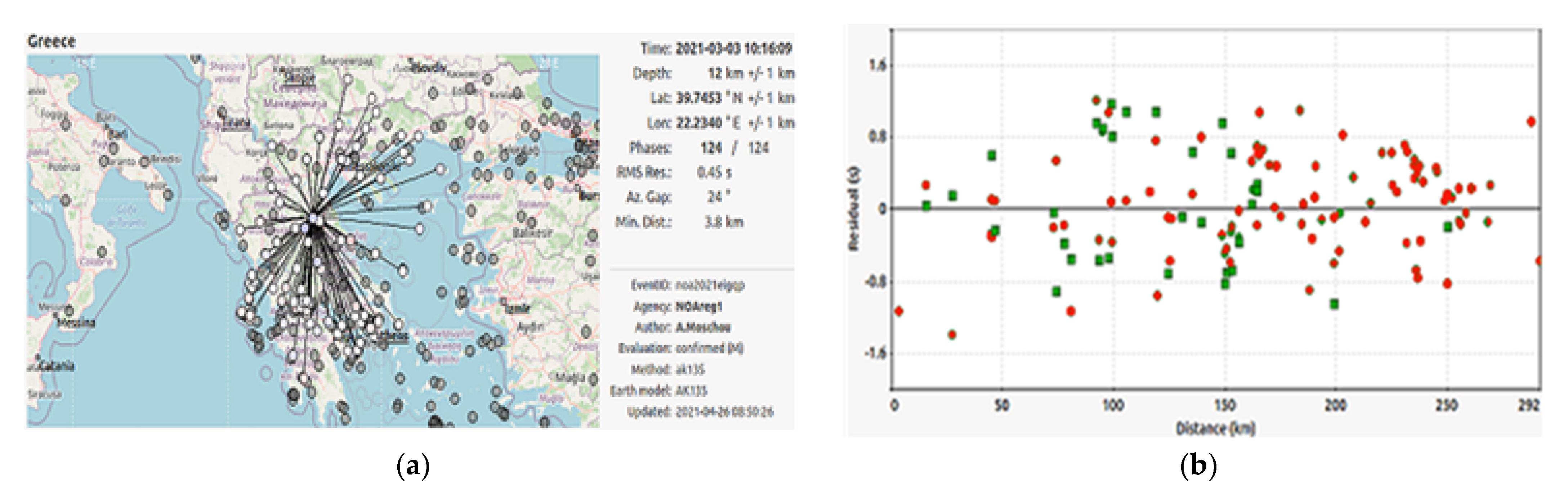
4.1.1. The Μ_L 6.0, Elassona, 3 March 2021 (10:16:08.3 UTC)

A strong earthquake, M_L = 6.0, occurred in the broader area of Thessaly, Central Greece, on 3 March 2021 (10:16:08.39, UTC). The geographical coordinates, as they were calculated manually for the scope of this study, were φ = 39.7453° Ν, λ = 22.2340° Ε at a depth of 12 km (Figure 5). The phases used to calculate the epicenter were 124 phases from P- and S-waves at epicentral distances between 3 and 265 km and an azimuthal gap of 24°. More distant stations indicated a longer extensive duration for P- and S-waves because of the simultaneous arrival of refracted and reflected P- and S-waves as well as sP-waves.

Figure 5a represents the geographical distribution of the stations that were used to calculate the epicenter, and Figure 5b shows a graph of the distance (km) versus residual (s) stations. Finally, the green circles denote the stations where only vertical components (P-waves) were used, while the green squares represent the stations where vertical and horizontal components (P-waves and S-waves) were used.

Figure 6 shows a section of the displacement record of the broadband seismological data from the mainshock. In local station records, both P and S direct-body waves exhibited durations shorter than 2 s.

The first strong aftershock occurred a few hours later at 11:45:45.99 (UTC) with a magnitude M_L = 5.1. A rich sequence followed these events, more specifically, from the main event’s time, and for the next 24 h, there were 268 seismic vibrations with a magnitude greater than 1 (Figure 7a). When monitoring the seismic sequence over the first month, 2268 aftershocks occurred, 34 with a magnitude M_L ≥ 4.0. The distribution of magnitudes concerning the number of earthquakes is presented in Figure 7a,b. As can be seen from the following diagrams, for the first day of the sequence, a significant number of earthquakes (~Nr = 268) were of a magnitude of 2.0 < M_L < 3.0, while over the first month, the number of the respective magnitudes that fluctuated was Νr = 2062.

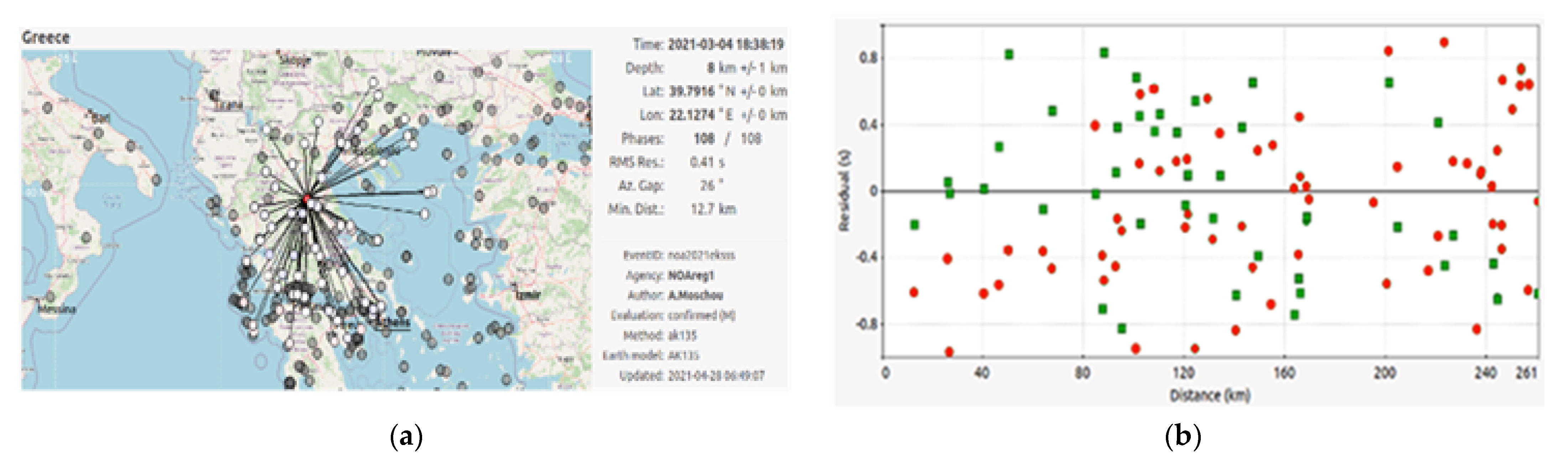
4.1.2. The Μ_L 5.9, Elassona, 4 March 2021 (18:38:19.1 UTC)

One day after the first event, a second (4 March, 18:38:19.1 UTC) event with a similar magnitude as the first (M_L 5.9) occurred on the NW section of the fault. The epicenter was determined to be 10 km north of the first mainshock (39.7916° N, 22.1274° E), while the depth was d = 8 km, as shown in Figure 8.

In calculating the epicenter, 108 phases were used from P- and S-waves at epicentral distances between 5 and 261 km and an azimuthal gap of 26°. More distant stations indicated a more extensive duration for P- and S-waves because of the simultaneous arrival of refracted and reflected P- and S-waves as well as sP-waves

4.2. Moment Tensor Solutions

The second goal of this study was to calculate the source parameters for the two strong and moderate events with a local magnitude Μ_L ≥ 4.0. The selected events presented a high signal-to-noise ratio, and we computed the moment tensor. Using the method of inversion for the seismic moment tensor, the Ammon code determined the seismic parameters [63]. It is noted that particular emphasis was given to stations close to the fault plane. However, due to their location, these stations contributed positively to the outcome of the inversion procedure.

Seismological broadband data (in epicentral distances, Δ < 6°) were selected and analyzed to determine the focal mechanism and the source parameters. In most cases, regional broadband data were selected, processed, and applied to the proposed methodology of at least six stations at an excellent azimuthal coverage. This was based on creating synthetic seismograms and directly comparing them with the observed ones for a given velocity structure. The reflectivity method of Kennett [64], as implemented by Randall [65], was used, and a bandpass filter was applied to the data. Filter frequencies varied depending on the type of waveform: a bandpass filter of 0.1–0.2 Hz corner frequencies for traces recorded by local stations and 0.01–0.1 Hz for regional waveforms. The same bandpass filter was applied both on the observed waveforms and synthetics, having a fixed length of 70 s. The next step was the deconvolution of the instrument response from the waveforms, and the waveform conversion through integration produced pure displacement. Finally, the horizontal components with rotation were converted to radial and transverse waveforms. The three previous displacement components must be cut in the same starting time (nearly 10 s before the first arrival) with a total duration of 300 s.

The inversion results indicate that inverting waveforms longer than 70 s resulted in higher misfits. The quality of the moment tensor solutions can be evaluated by considering the average misfit and the compensated linear vector dipole (CLVD). A quality code consists of the letters A–D [65] for each solution for the minimum misfit and between the numbers 1 and 4 for the percent of CLVD [66].

The results of the inversion for the two main events as well as their comparison with those of other institutes/universities, are presented in Table 2. Only the DC part of the moment tensors is discussed because we did not consider the CLVD parts as having a physical meaning.

4.2.1. The Μ_w 6.3, Elassona, 3 March 2021 (10:16:08.3 UTC)

We applied the proposed methodology to examine the active fault that ruptured on the 3 March, the mainshock, the type of focal mechanism, and the source parameters. 21 seismological records were used in the final solution at seven broadband stations with epicentral distances between 70 and 280 km, having an adequate azimuthal distribution (maximum gap of 70°) and covering all quadrants of different polarity on the focal sphere to constrain the nodal planes. The waveform inversion indicated the activation of a normal type faulting with source parameters equal to φ = 147°, δ = 57°, and λ = −86°; the depth was calculated at d = 11 km; the seismic moment was M = 3.173e+25 dyn*cm. In addition, this technique showed a high percentage of double pairs of forces concerning the double vector dipole with DC = 85% and CLVD = 15%.

The obtained focal mechanism was found to be in good agreement with the one proposed solution by the USGS (Table 2). The focal mechanism of an earthquake and the simulation of seismic waves for the selected stations are presented in Figure 9.

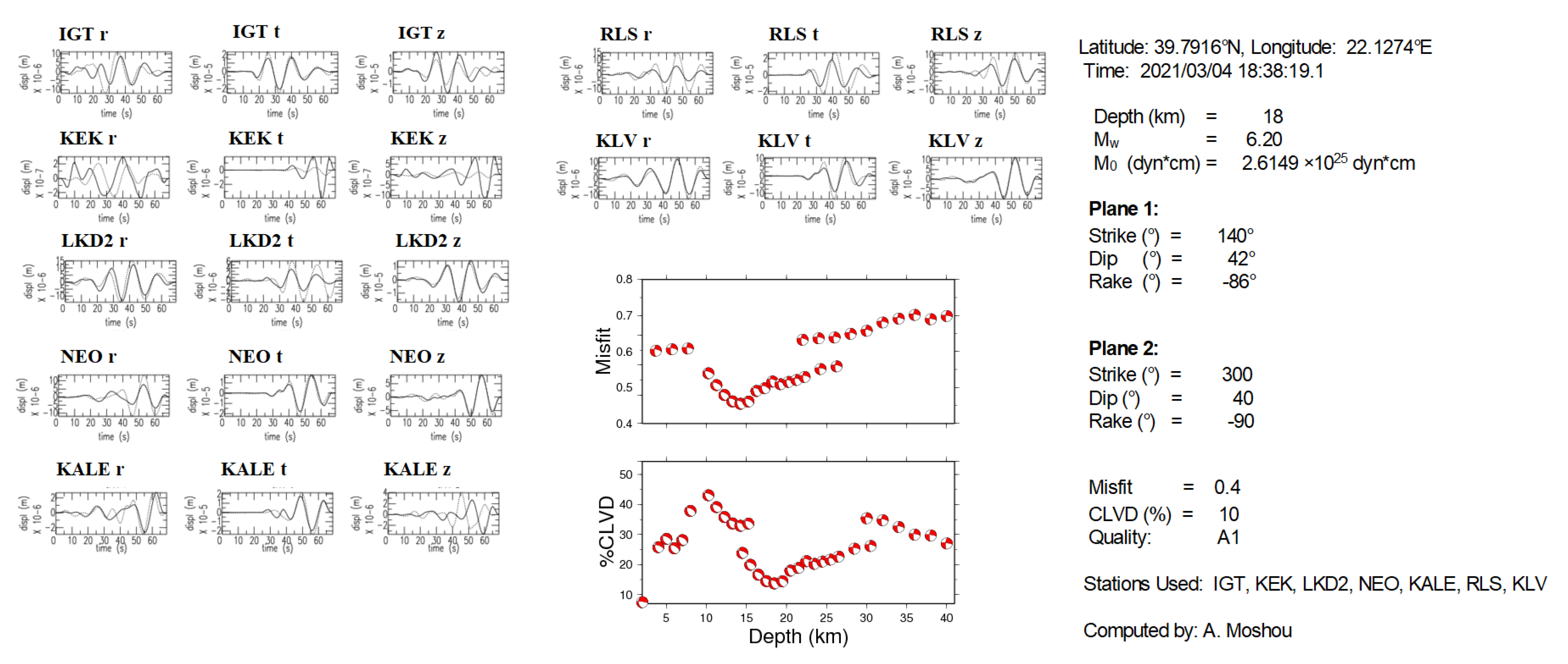
4.2.2. The Μ_w 6.2, Elassona, 4 March 2021 (18:38:19.1 UTC)

On 4 March 2021 (18:38:19.1, UTC), an extreme event with a similar magnitude occurred in the same region one day later. It applied the same methodology with the same criteria, as the two events had similar magnitude and waveforms. The focal mechanism was also a normal faulting plane solution with directivity on the east–northeast–west-southwest-oriented planes and closely matched the observed first-motion body-wave polarities. The seismic moment magnitude was calculated as M_w = 6.2, with the likely fault plane having the strike of φ = 140°, the dip of δ = 42°, and the rake of λ = −86°. The following calculations of other agencies for the mainshock indicated pure NW-SE normal dip-slip faulting. The calculated depth from moment tensor inversion was 18 km (Figure 10). The focal mechanism was found to be in good agreement with the one proposed solution by the GFZ (Table 2).

Various seismological observatories and institutes routinely publish moment tensor solutions for strong events in Greece. Therefore, the German Research Centre for Geosciences (GFZ), the United States Geological Survey (USGS), the National Institute of Geophysics and Volcanology (INGV), the Kandilli Observatory and Earthquake Research Institute (KOERI), and others, as shown in Table 2, were selected in the present study to compare their solutions with those derived from this work. In addition, ordinary moment tensor solutions were available from the European–Mediterranean Seismological Centre [4], and a comparison of the moment magnitude (M_w) and focal mechanism results was performed.

5. Discussion

The historical seismicity of the region of Thessaly is related to the North Transform Fault (NTF), approximately 50 km southeast of the double earthquake. Therefore, knowledge regarding a dynamic error in this area is minimal. Thessaly, Central Greece, is a region of active crustal extension but low strain [67]. This was confirmed both empirically and by the study in [68]. Although the Thessaly region has a well-known history of large earthquakes, the studied region showed only weak seismicity over the last 15 years, which the Hellenic Unified Seismological Network covers. A subcrustal presence suggests that the upper crust deformation was probably caused by large-scale tectonics and plate dynamics.

On 3–4 March, two similar magnitudes (M_w = 6.3 and 6.2, respectively) occurred in the broader area of the Thessaly area. A few hours later, two earthquakes with similar magnitudes (M_w = 5.3 and 5.2, respectively) were observed in the same region. A rich seismic sequence followed these earthquakes. More specifically, in the first month alone, 2062 earthquakes took place. We used the Hellenic Unified Seismological Network (HUSN) (Figure 2) to study the two 2021 earthquakes in the Elassona in Thessaly, Central Greece. We accurately calculated the epicenter of these two events and computed the moment tensor of the mainshock and other more significant magnitude aftershocks. Two datasets were used for inversion: one using regional stations and the other including only stations close to the mainshock’s epicenter. These analyses show that the observed inversion indicates the activation of a normal type faulting and shallow depth for both events.

The first-motion body-wave polarities provide information only regarding the onset of the rupture, whereas the inversion of surface waveforms includes information regarding the earthquake centroid (point of highest slip release). Especially for more significant earthquakes, these two points do not necessarily coincide spatially. According to the study in [67], resolving moment tensors, especially strike-slip mechanisms, is challenging when the source depth is much shallower than the wavelength considered during inversion. On the contrary, this is not always the case for moderate events due to the extensive period component’s poor quality. Analysis of moderate events is crucial for seismogenic volumes, where many such earthquakes occur, allowing the calculation of their source parameters. Thus, the seismotectonic characteristics of the study area can be determined. Knowing the source parameters for moderate earthquakes is very important for seismically active regions, mainly when no significant events occur. In general, it allows analytical studies to reveal a specific area’s tectonics and seismogenic characteristics. In the present work, the applied waveform inversion methodology was calculated using data at regional distances, the source parameters for the most decisive events, and 33 moderate earthquakes with magnitudes of M_w > 4.0. Finally, the results for the moment tensor solutions of the analyzed aftershocks are shown in Appendix A.

Almost all aftershocks of the sequence occurred north of the surface rupture. Interestingly, the aftershocks were concentrated along the edges of the presumptive rupture plane. This effect is visible on the map view as a gap of aftershocks north of the central part of the surface rupture. The seismicity gap is visible at the shallow depth of the first mainshock on the east-west depth section. Considering only the aftershocks that occurred in March 2021, they spread in the east-west direction. From the different depths for the first mainshock and the east-west extent of the aftershock distribution, we estimated the size of the rupture plane and recorded and visualized its spreading.

Figure 11 represents the relation time versus the event’s magnitude in the study area. It was observed that most aftershocks occurred within the first three months in the first 75 days. It was observed that for the first two months after the occurrence of the main earthquake, both the density and magnitude of the aftershocks were much higher than the rest.

Figure 12 represents the relation distance from the mainshock versus the event’s magnitude in the Elassona, Central Greece study area. From the diagram, one can observe that a higher density of epicenters accumulated in the first 20 km from the epicenter of the main earthquake. Magnitude variations ranged from 1.0 < M_L < 4.0, as when seismic monitoring stations are added or removed, our ability to detect small earthquakes changes reliably.

The seismic sequence’s monitoring and study showed a shift in the epicenters to the northwest (Figure 13 and Figure 14). The spatial distribution versus date indicated a displacement of earthquake density to the NW of the first three dates after the main event. Then, the density of the earthquakes decreased, and after eight days, a high-density event occurred at latitude = 39.80° and longitude = 21.90°, without any further indication of spatial displacement. This fact proves the claim that the two strong earthquakes belonged to two different fault zones.

We determined deviatoric moment tensor solutions for 34 earthquakes with M_w ≥ 4.0 at depths between 6 and 14 km. The depths decreased in the eastern and especially in the western termination of the sequence. The proposed methodology’s application gave rise to the activation of normal faulting with the direction N-S. The depth varied 11 km < d < 15 km for the five strongest sequences, a fact that agrees with the study in [67], while the magnitudes were 5.2 < Μ_w < 6.3. Here, they were concentrated at approximately 7 km in depth, in contrast to about 14 km in the central part of the sequence. The aftershocks occurred along the entire surface rupture length but mainly north. A very high percentage of a double couple (DC) in relation emerged to the compensated linear vector dipole (CLVD) for the most significant percentage of solutions. More specifically, 80% of the solutions presented a DC > 90% solution, while the remaining 20% had a DC between 75% and 89%. The focal mechanism solutions for the strongest earthquakes determined in this study appear in Figure 15.

6. Conclusions

Thessaly (Central Greece) experienced a rich seismic sequence in March 2021. The mainshock, measuring M_L = 6.3, struck on 3 March and was quickly followed by a powerful aftershock, measuring M_L = 6.2. Using a large dataset, high-resolution catalogs of earthquakes, and hundreds of focal mechanisms, we provided a thorough investigation of the March–April 2021 seismic sequence in Northern Thessaly (Damasi–Tyrnavos region). More than 30 focal mechanisms for earthquakes with M 4.0 were computed using local–regional data. The occurrences primarily showed normal faulting in an NW-SE direction, but there was also evidence of WNW-ESE to E-W normal faulting, especially after the last significant event on 12 March 2021. The aftershocks’ spatial distribution and focal mechanisms indicated normal faulting with a strike direction of NW-SE.

Additionally, the focal mechanisms indicated an extensional stress field oriented differently than previously known, from NE to SW. Strong evidence points to the rupture of two neighboring fault segments based on the two most significant shocks’ size, location, and spatiotemporal evolution. We propose that this fault system, a steeper splay of a deeper low-to-moderate angle normal fault, was partially reactivated as a secondary surface rupture throughout the episode.

For the study period, more than 3,500 events were recorded and analyzed. The spatial distribution and the timely distribution of high-density aftershocks indicate the activation of two different fault zones. The depth value varied between 10 and 15 km for the aftershocks where the source parameters were calculated. The error depth was ~1 km; the depth error depended on various factors such as the software used, the velocity model, the number of available stations, the azimuth distribution of the existing stations, and the analyst’s ability.

For the first two months after the main earthquake, the density and magnitude of the aftershocks were much higher than the rest. A higher density of epicenters accumulates in the first 20 km from the epicenter of the main earthquake. Magnitude variations were 1.0 < M_L < 4.0.

According to our findings, the 2021 doublet ruptured previously unmapped fault segments, with most of the slide occurring during the two big shocks to the west of Tyrnavos town. From the first main shock’s epicenter, the activity predominantly moved northward, rupturing a crustal volume between 4 and 15 km thick and producing shallower off-fault seismicity.

References

1. Hatzfeld, D.; Ziazia, M.; Kementzetzidou, D.; Hatzidimitriou, P.; Panagiotopoulos, D.; Makropoulos, K. Microseismicity and focal mechanisms at the western termination of the North Anatolian Fault and their implications for continental tectonics. Geophys. J. Int. 1999, 137, 891–908. [Google Scholar] [CrossRef]
2. Kahle, H.-G.; Cocard, M.; Pete, Y.; Geiger, A.; Reilinger, R.P.; Barka, A.; Veis, G. GPS-derived strain rate field within the boundary zones of the Eurasian, African and Arabian Plates. J. Geophys. Res. 2000, 105, 23353–23370. [Google Scholar] [CrossRef]
3. Caputo, R.; Pavlides, S. Late Cenozoic geodynamic evolution of Thessaly and surroundings (Central-Northern Greece). Tectonophysics 1993, 223, 339–362. [Google Scholar] [CrossRef]
4. Emsc-csem.org. Earthquakes—Earthquake today—Latest Earthquakes in the World—EMSC. 2022. Available online: https://www.emsc-csem.org/#2 (accessed on 11 May 2022).
5. Lekkas, E.; Agorastos, K.; Mavroulis, S.; Kranis, C.; Skourtsos, E.; Carydis, P.; Thoma, T. The early March 2021 Thessaly earthquake sequence. Newsl. Environ. Disaster Cris. Manag. Strateg. 2021, 22, ISSN 2653–9454. Available online: https://www.researchgate.net/publication/350091329_The_early_March_2021_Thessaly_Greece_earthquake_sequence (accessed on 8 June 2022).
6. Zouros, N.; Pavlides, S.; Chatzipetros, A. Recent movement on the Larissa plain neotectonic faults (Thessaly, C. Greece). Water-level fluctuation or tectonic creep. In Proceedings of the ESC XXIV General Assembly, Athens, Greece, 19–24 September 1994; Volume 67. [Google Scholar]
7. Soulios, G. Subsidence de terrains alluviaux dans le sud-est de la plaine de Thessalie, Grece. In Engineering Geology and the Environment; Marinos, P.G., Koukis, G.C., Tsiambas, G.C., Stournaras, G.C., Eds.; A.A. Balkema, Brookfield: Rotterdam, The Netherlands, 1997; pp. 1067–1072. [Google Scholar]
8. Rapti-Caputo, D.; Caputo, R. Some remarks on the formation of ground fissures in Thessaly, Greece. In Proceedings of the 5th International Symposium on Eastern Mediterranean Geology, Thessaloniki, Greece, 14–20 April 2004; pp. 1016–1019. [Google Scholar]
9. Kontogianni, V.; Pytharouli, S.; Stiros, S. Ground subsidence, Quaternary faults and vulnerability of utilities and transportation networks in Thessaly, Greece. Environ. Geol. 2007, 52, 1085–1095. [Google Scholar] [CrossRef]
10. Apostolidis, E.; Koukis, G. Engineering-geological conditions of the formations in the Western Thessaly basin, Greece. Cent. Eur. J. Geosci. 2013, 5, 407–422. [Google Scholar] [CrossRef] [Green Version]
11. Ilia, I.; Loupasakis, C.; Tsangaratos, P. Assessing ground subsidence phenomena with persistent scatterer interferometry data in western Thessaly, Greece. Bull. Geol. Soc. Greece 2016, 50, 1693–1702. [Google Scholar] [CrossRef]
12. Georgoulas, G.; Konstantaras, A.; Katsifarakis, E.; Stylios, C.D.; Maravelakis, E.; Vachtsevanos, G.J. “Seismic-mass” density-based algorithm for spatio-temporal clustering. Expert Syst. Appl. 2013, 40, 4183–4189. [Google Scholar] [CrossRef]
13. Konstantaras, A.J.; Katsifarakis, E.; Maravelakis, E.; Skounakis, E.; Kokkinos, E.; Karapidakis, E. Intelligent Spatial-Clustering of Seismicity in the Vicinity of the Hellenic Seismic Arc. Earth Sci. Res. 2012, 1, 1–10. [Google Scholar] [CrossRef] [Green Version]
14. Konstantaras, A. Deep Learning and Parallel Processing Spatio-Temporal Clustering Unveil New Ionian Distinct Seismic Zone. Informatics 2020, 7, 39. [Google Scholar] [CrossRef]
15. Kagan, Y.Y. 3-D rotation of double-couple earthquake sources. Geophys. J. Int. 1991, 106, 709–716. [Google Scholar] [CrossRef]
16. Konstantaras, A.; Vallianatos, F.; Varley, M.R.; Makris, J.P. Soft-Computing Modelling of Seismicity in the Southern Hellenic Arc. IEEE Geosci. Remote Sens. Lett. 2008, 5, 323–327. [Google Scholar] [CrossRef]
17. Astiz, L.; Kanamori, H. An earthquake doublet in Ometepec, Guerro, Mexico. Phys. Earth Planet. Inter. 1984, 34, 24–45. [Google Scholar] [CrossRef]
18. Poupinet, G.; Ellsworth, W.L.; Frechet, J. Monitoring Velocity Variations in the Crust Using Earthquake Doublets: An Application to the Calaveras Fault, California. J. Geophys. Res. Atmos. 1984, 89, 5719–5731. [Google Scholar] [CrossRef] [Green Version]
19. Beroza, G.C.; Spudich, P. Linearized inversion for fault rupture behavior: Application to the 1984 Morgan Hill, California, earthquake. J. Geophys. Res 1988, 93, 6275–6296. [Google Scholar] [CrossRef]
20. Felzer, K.R.; Becker, T.W.; Abercrombie, R.E.; Ekström, G.; Rice, J.R. Triggering of the 1999 MW 7.1 Hector Mine earthquake by aftershocks of the 1992 MW 7.3 Landers earthquake. J. Geophys. Res. 2002, 107, 2190. [Google Scholar] [CrossRef]
21. Bath, M. Earthquake energy and magnitude. Phys. Chem. Earth 1966, 7, 117–165. [Google Scholar] [CrossRef]
22. Richter, C.F. Elementary Seismology; Freeman & Co.: San Francisco, CA, USA, 1958. [Google Scholar]
23. Kagan, Y.; Jackson, D. Worldwide doublets of large shallow earthquakes. Bull. Seismol. Soc. Am. 1999, 89, 1147–1155. [Google Scholar] [CrossRef]
24. Konstantaras, A.J. Classification of Distinct Seismic Regions and Regional Temporal Modelling of Seismicity in the Vicinity of the Hellenic Seismic Arc. IEEE J. Sel. Top. Appl. Earth Obs. Remote Sens. 2012, 6, 1857–1863. [Google Scholar] [CrossRef]
25. Konstantaras, A. Expert knowledge-based algorithm for the dynamic discrimination of interactive natural clusters. Earth Sci. Inform. 2016, 9, 95–100. [Google Scholar] [CrossRef]
26. Moshou, A. Strong Earthquake Sequences in Greece during 2008-2014: Moment Tensor Inversions and Fault Plane Discrimination. Open J. Earthq. Res. 2020, 9, 323–348. [Google Scholar] [CrossRef]
27. Moshou, A.; Argyrakis, P.; Konstantaras, A.; Daverona, A.-C.; Sagias, N.C. Characteristics of Recent Aftershocks Sequences (2014, 2015, 2018) Derived from New Seismological and Geodetic Data on the Ionian Islands, Greece. Data 2021, 6, 8. [Google Scholar] [CrossRef]
28. Bbnet.gein.noa.gr. NOA Seismic Network (HL)—Introduction. 2022. Available online: https://bbnet.gein.noa.gr/HL (accessed on 15 March 2022).
29. Geophysics.geo.auth.gr. Τομέας Γεωφυσικής A.Π.Θ. 2022. Available online: http://geophysics.geo.auth.gr (accessed on 15 March 2022).
30. Seiscomp.de. Scolv—SeisComP Release Documentation. 2022. Available online: https://www.seiscomp.de/doc/apps/scolv.html (accessed on 15 March 2022).
31. Seiscomp.de. 2022. Available online: https://docs.gempa.de/seiscomp3/current/apps/scolv.html (accessed on 25 April 2022).
32. Haslinger, F.; Kissling, E.; Ansorge, J.; Hatzfeld, D.; Papadimitriou, E.; Karakostas, V.; Makropoulos, K.; Kahle, H.; Peter, Y. 3D crustal structure from local earthquake tomography around the Gulf of Arta (Ionian region, NW Greece). Tectonophysics 1999, 304, 201–218. [Google Scholar] [CrossRef]
33. Kanamori, H. Determination of effective tectonic stress associated with earthquake faulting. The Tottori earthquake of 1943. Phys. Earth Planet. Inter. 1972, 5, 426–434. [Google Scholar] [CrossRef]
34. Haskell, N. Total energy and energy spectral density of elastic wave radiation from propagating faults. Bull. Seismol. Soc. Am. 1964, 54, 1811–1841. [Google Scholar] [CrossRef]
35. Helmberger, D.V. Theory and application of synthetic seismograms. In Proceedings of the International School of Physics <<Enrico Fermi>>, Course LXXXV. pp. 174–222. 1983. Available online: https://eurekamag.com/research/020/477/020477221.php (accessed on 8 June 2022).
36. Langston, C. A body wave inversion of the Koyna, India, earthquake of December 10, 1967, and some implications for body wave focal mechanisms. J. Geophys. Res. 1976, 81, 2517–2529. [Google Scholar] [CrossRef] [Green Version]
37. Golub, H.; Van, L.C. Matrix Computations; The Johns Hopkins Univeristy Press: Baltimore, Maryland, 1983; p. 476. [Google Scholar]
38. Das, S.; Kostrov, B. Inversion for seismic slip rate history and distribution with stabilizing constraints: Application to the 1986 Andreanof Islands Earthquake. J. Geophys. Res. 1990, 95, 6899. [Google Scholar] [CrossRef]
39. Brune, J. Tectonic stress and the spectra of seismic shear waves from earthquakes. J. Geophys. Res. 1970, 75, 4997–5009. [Google Scholar] [CrossRef] [Green Version]
40. Langston, C. Source inversion of seismic waveforms: The Koyna, India, earthquakes of 13 September 1967. Bull. Seismol. Soc. Am. 1981, 71, 1–24. [Google Scholar] [CrossRef]
41. Langston, C.; Barker, J.; Pavlin, G. Point-source inversion techniques. Phys. Earth Planet. Inter. 1982, 30, 228–241. [Google Scholar] [CrossRef]
42. Cotton, F.; Campillo, M. Frequency domain inversion of strong motions: Application to the 1992 Landers earthquake. J. Geophys. Res. Solid Earth 1995, 100, 3961–3975. [Google Scholar] [CrossRef]
43. Kiratzi, A.; Sokos, E.; Ganas, A.; Tselentis, A.; Benetatos, C.; Roumelioti, Z.; Serpetsidaki, A.; Andriopoulos, G.; Galanis, O.; Petrou, P. The April 2007 earthquake swarm near Lake Trichonis and implications for active tectonics in western Greece. Tectonophysics 2008, 452, 51–65. [Google Scholar] [CrossRef]
44. Usgs.gov. 2022. FPFIT, FPPLOT and FPPAGE; Fortran Computer Programs for Calculating and Displaying Earthquake Fault-plane Solutions | U.S. Geological Survey. Available online: https://www.usgs.gov/publications/fpfit-fpplot-and-fppage-fortran-computer-programs-calculating-and-displaying (accessed on 8 June 2022).
45. Hardebeck, J.L.; Shearer, P.M. A New Method for Determining First-Motion Focal Mechanisms. Bull. Seismol. Soc. Am. 2002, 92, 2264–2276. [Google Scholar] [CrossRef] [Green Version]
46. Meju, M. Geophysical Data Analysis: Understanding Inverse Problem Theory and Practise; Course Notes Series; Society of Exploration Geophysicists: Houston, TX, USA, 1994; Volume 6. [Google Scholar]
47. Aki, K.; Richards, P.G. Quantitative Seismology, 2nd ed.; Freeman: San Francisco, CA, USA, 1980. [Google Scholar]
48. Dreger, D. Time—Domain Moment Tensor INVerse Code (TDMT_INV) Version 1.1; Berkley Seismological Laboratory: Berkeley, CA, USA, 2002; p. 18. [Google Scholar]
49. Ichinose, G. Source Parameters of Eastern California and Western Nevada Earthquakes from Regional Moment Tensor Inversion. Bull. Seismol. Soc. Am. 2003, 93, 61–84. [Google Scholar] [CrossRef]
50. Bouchon, M. A simple method to calculate Green’s functions for elastic layered media. Bull. Seismol. Soc. Am. 1981, 71, 959–971. [Google Scholar] [CrossRef]
51. Bouchon, M. A Review of the Discrete Wavenumber Method. Pure Appl. Geophys. 2003, 160, 445–465. [Google Scholar] [CrossRef]
52. Bouchon, M.; Aki, K. Discrete wave-number representation of seismic-source wave fields. Bull. Seismol. Soc. Am. 1977, 67, 259–277. [Google Scholar] [CrossRef]
53. Bouchon, M. Discrete wave number representation of elastic wave fields in three-space dimensions. J. Geophys. Res. Solid Earth 1979, 84, 3609–3614. [Google Scholar] [CrossRef]
54. Athanasiadis, C.; Martin, P.; Spyropoulos, A.; Stratis, I. Scattering relations for point sources: Acoustic and electromagnetic waves. J. Math. Phys. 2002, 43, 5683–5697. [Google Scholar] [CrossRef] [Green Version]
55. Athanasiadis, C. On the acoustic scattering amplitude for a multi-layered Scatterer. J. Aust. Math. Soc. Appl. Math. 1998, 39, 431–448. [Google Scholar] [CrossRef] [Green Version]
56. Herrmann, R.B.; Wang, C.Y. A comparison of synthetic seismograms. Bull. Seismol. Soc. Am. 1985, 75, 41–56. [Google Scholar] [CrossRef]
57. Jost, M.; Hermann, R. A student’s Guide to and Review of Moment Tensors. Seismol. Res. Lett. 1989, 60, 37–57. [Google Scholar] [CrossRef]
58. Tarantola, A.; Valette, B. Inverse Problems = Quest for Information. J. Geophys. 1982, 50, 159–170. [Google Scholar]
59. Tarantola, A.; Valette, B. Generalized Nonlinear Inverse Problems Solved Using the Least Squares Criterion. Rev. Geophys. Space Phys. 1982, 20, 219–232. [Google Scholar] [CrossRef]
60. Moser, T.J.; Van Eck, T.; Nolet, G. Hypocenter determination in strongly heterogeneous Earth models using the shortest path method. J. Geophys. Res. 1992, 97, 6563–6572. [Google Scholar] [CrossRef]
61. Wittlinger, G.; Herquel, G.; Nakache, T. Earthquake location in strongly heterogenous media. Geophys. J. Int. 2007, 115, 759–777. [Google Scholar] [CrossRef] [Green Version]
62. Lomax, A.; Virieux, J.; Volant, P.; Berge-Thierry, C. Probabilistic earthquake location in 3D and layered models: Introduction of a Metropolis-Gibbs method and comparison with linear locations. In Advances in Seismic Event Location; Thurber, C.H., Rabinowitz, N., Eds.; Kluwer: Amsterdam, The Netherlands, 2000; pp. 101–134. [Google Scholar]
63. Ammon, C.J.; Randall, G.E.; Zandt, G. On the non-uniqueness of receiver function inversions. J. Geophys. Res. 1990, 95, 15303–15318. [Google Scholar] [CrossRef]
64. Kennett, B.N.L. Seismic Wave Propagation in Stratified Media; Cambridge University Press: Cambridge, UK, 1983. [Google Scholar]
65. Randal, G.E. Efficient calculation of complete differential seismograms for laterally homogeneous earth models. Geophys. J. Int. 1994, 118, 245–254. [Google Scholar] [CrossRef] [Green Version]
66. Konstantinou, K.; Melis, N.; Boukouras, K. Routine Regional Moment Tensor Inversion for Earthquakes in the Greek Region: The National Observatory of Athens (NOA) Database (2001–2006). Seismol. Res. Lett. 2010, 81, 750–760. [Google Scholar] [CrossRef]
67. Tolomei, C.; Caputo, R.; Polcari, M.; Famiglietti, N.A.; Maggini, M.; Stramondo, S. The Use of Interferometric Synthetic Aperture Radar for Isolating the Contribution of Major Shocks: The Case of the March 2021 Thessaly, Greece, Seismic Sequence. Geosciences 2021, 11, 191. [Google Scholar] [CrossRef]
68. De Novellis, V.; Reale, D.; Adinolfi, G.; Sansosti, E.; Convertito, V. Geodetic Model of the March 2021 Thessaly Seismic Sequence Inferred from Seismological and InSAR Data. Remote Sens. 2021, 13, 3410. [Google Scholar] [CrossRef]
Figure 1. General structure map of Thessaly. The red circles represent the prefectures; red lines indicate the main active faults for the study area; the six yellow stars indicate the historical earthquake in the broader area of Thessaly; the blue lines represent rivers.
Applsci 12 07446 g001
Figure 2. Geographical distribution of the Hellenic Unified Seismological Network’s stations in the region of Thessaly. Green triangles represent the seismological stations belonging to the University of Patras, purple triangles denote the portable network installed by the Aristotle University of Thessaloniki immediately after the earthquake, and the red triangles are the stations of the National Observatory of Athens. The light blue color represents the cities near the epicenter.
Applsci 12 07446 g002
Figure 3. Elementary focal mechanisms.
Applsci 12 07446 g003
Figure 4. Black lines correspond to the main active faults for the study area—a general seismicity map of the broader area of the Thessalian, Central Greece. Light blue rectangles denote the cities of the study area. The stars represent the events in the study area for 3 March 2021–31 December 2021.
Applsci 12 07446 g004
Figure 5. (a) Azimuthal distribution of the stations used to calculate the epicenter of the 3 March 2021 (10:16:08.39, UTC) and the characteristics of the solution; (b) graph of the distance (km)–residual (s) stations. The green squares represent the stations where only vertical components (P-waves) were used, while the red circles represent the stations where both vertical and horizontal components (P-waves and S-waves) were used.
Applsci 12 07446 g005
Figure 6. A section of the displacement record of the stations. The horizontal components (east–west and north–south traces) were rotated into radial and transverse components. The sP-wave was clear in the radial and vertical components, but only the S-wave was observed along with the surface waves in the transverse component.
Applsci 12 07446 g006
Figure 7. (a) Magnitude distribution of the aftershocks recorded for the first 24 h after the ML 6.0, number of events (Nr) = 268; (b) the distribution of magnitudes concerning the number of earthquakes for the first month after the main event. Nr = 2062.
Applsci 12 07446 g007
Figure 8. (a) Azimuthal distribution of the stations used to calculate the epicenter of the 4 March 2021 (18:38:19.19, UTC) and the characteristics of the solution; (b) graph of the distance (km)–residual (s) stations. The green squares represent the stations where only vertical components (P-waves) were used, while the red circles represent the stations where vertical and horizontal components (P-waves and S-waves) were used.
Applsci 12 07446 g008
Figure 9. Inversion results for the first mainshock of 3 March 2021 (10:16:08.3 UTC). The left of the misfit/CLVD diagrams observed and synthetic displacement waveforms (continuous and dotted lines, respectively) are shown at the inverted stations for the radial, tangential, and vertical components. The solution’s summary and the fault plane solution as a lower hemisphere equal-area projection are depicted in the right part of the figure.
Applsci 12 07446 g009
Figure 10. Inversion results for the second major mainshock of 4 March 2021 (18:38:19.19 UTC). To the left of the misfit/CLVD diagrams, observed and synthetic displacement waveforms (continuous and dotted lines, respectively) are shown at the inverted stations for the radial, tangential and vertical components. The solution’s summary and the fault plane solution as a lower hemisphere equal-area projection are depicted in the right part of the figure.
Applsci 12 07446 g010
Figure 11. Distribution of magnitudes with time as a function of days from the mainshock of 3 March 2021 (10:16:08, UTC) for the 3787 records. On the x-axis is the magnitude time (days from mainshock) of each event from Elassona, Central Greece, while on the y-axis is the local magnitude (ML).
Applsci 12 07446 g011
Figure 12. Location with distance (km) from mainshock as a magnitude (ML) function for the 3.787 events recorded. On the x-axis is the distance from the mainshock, while on the y-axis is the magnitude of each aftershock.
Applsci 12 07446 g012
Figure 13. Spatial distribution (longitude) of earthquake density for different dates.
Applsci 12 07446 g013
Figure 14. Spatial distribution (latitude) of earthquake density for different dates.
Applsci 12 07446 g014
Figure 15. A seismotectonic map of the study area. On the map, the epicenters appear for the study area’s more significant events, corresponding focal mechanisms, and significant faults.
Applsci 12 07446 g015