Identification of Areas of Anomalous Tremor of the Earth’s Surface on the Japanese Islands According to GPS Data

Abstract

Statistical properties of Earth surface tremors measured by means of GPS were investigated. This article considers measurements of the Earth’s surface displacements in three orthogonal directions relayed by a network of GPS sensors with about 1200 points distributed across Japan in 2009–2021. Next, the following characteristics of the tremors were considered: the entropy of the distribution of squared orthogonal wavelet coefficients, the entropy of the distribution of power spectrum values, and the spectral index. The anomalous regions of maxima of probability densities of the distribution of extreme values of the tremor statistics were determined: entropy minima and spectral index maxima. The average density maps of the distribution of extreme value tremor statistics were found to be highly correlated with one another. This made it possible to consider a weighted average density map and identify five anomalous regions in the center and south of Japan. A trajectory of visiting anomalous regions by a sequence of points realizing local maxima of the average probability density was obtained, for which seasonal periodicity was set. Estimates of changes in the average and maximum values of the correlation coefficients of tremor properties in an auxiliary network of 16 reference points in a semi-annual time window were obtained.

1. Introduction

Analysis of the spectral structure and models of the noise component of a GPS time series is traditionally of interest to researchers. In [1], spectral indexes were analyzed by fitting power laws to spectra and estimating their parameters using the maximum likelihood method. The effect of the flicker noise intensity of a GPS time series on velocity determination errors, depending on the measurement latitude, was studied in [2,3]. In [4,5,6], the maximum likelihood method was applied to estimate the amplitudes of GPS time series noise component models for various regions of the world. The problem of estimating the error in determining the velocity based on the spectral index was considered in [7].

The use of parametric models of a GPS time series to consider the effect of gaps in data for tectonically active regions is described in [8]. In [9,10] the high-frequency noise structure of a GPS time series for a number of areas in New Zealand and the United States was analyzed. The influence of the seasonal component of the hydrological load on the Earth’s surface on the determination of the velocities of tectonic plates was studied in [11,12]. The extraction of common spatial characteristics and seasonal components of a GPS time series using the principal component method, empirical orthogonal functions, and singular spectrum analysis was considered in [13,14]. In [15], the high-frequency noise of a GPS time series was analyzed together with the records of the seismic network of accelerometers.

The relationship between the appearance of non-stationary effects in the GPS time series and the processes of slow motions at the boundaries between crustal blocks was analyzed in [16]. Estimates of the non-stationary effects of GPS time series and station positioning stability using discrete wavelet transforms were considered in [17,18]. In [19,20], the coherence of the tremors of the Earth’s surface measured by GPS was studied. An assessment of the fractal characteristics of a high-frequency GPS time series to identify potentially dangerous seismically active regions in Japan and California was used in [21,22,23].

This article analyzes the structure of high-frequency noise in the time series of the network of GPS stations in Japan (about 1200 points) over 13 years of observations, 2009–2013, with a time step of 5 min. Four characteristics of tremors are considered: the entropy of the distribution of squared orthogonal wavelet coefficients, the entropy of the distribution of power spectrum values, and two estimates of the spectral index, which is understood as the regression coefficient between the logarithm of the power spectrum and the logarithm of the period. The first estimate of the spectral index is traditional, by calculating the power spectrum. Another estimate of the slope is based on orthogonal wavelet decompositions, where the averages of the squares of the wavelet coefficients are considered as the contribution of the frequency band of the detail level of the decomposition to the total signal energy. For successive time fragments 1 day long (288 readings with a time step of 5 min), for measurements at each station, the values of the four statistics described above are calculated after detrending by a 4th order polynomial. The removal of the trend is aimed at getting rid of the influence of external deterministic factors, such as tidal and thermal deformations, and switching to the analysis of the random high-frequency component of the Earth’s surface displacements, which we will call tremors. The anomalous regions of maxima of probability densities of the distribution of extreme values of the studied tremor statistics are determined: entropy minima and spectral index maxima. This definition of tremor anomalous behavior is based on the fact that white noise is characterized by maximum entropy values and a zero spectral index. Consequently, the maximum deviation from uninformative “white-noise” behavior should be characterized by entropy minima and spectral slope maxima.

2. Materials and Methods

Ground displacement data measured by GPS are taken from the website [24]. These data represent displacements of the Earth’s surface in three orthogonal directions, which we will further denote as E, N, and Up for displacements in the west-east, north-south and vertical directions, with a time step of 5 min [25].

Figure 1a shows the positions of GPS points for measuring displacements of the Earth’s surface, as well as 16 numbered reference points. These points will be further needed to assess the spatial correlations between the properties of the Earth’s surface tremors. Reference point positions were noted as the centers of 16 clusters of GPS stations using the K-means method [26]. The numbering was performed by decreasing the latitude of the reference points. Figure 1b presents the density of GPS stations, which were estimated by Gaussian kernel method [26] with bandwidth 0.5° (≈56 km), within a regular 30 × 30 network of nodes which covered the region. Figure 1c shows a graph of the daily number of operational GPS stations for 13 years of observations, 2009–2021.

By operational stations on the current day, we mean those stations for which the total number of missing data does not exceed 10% of the duration of the daily window of 288 counts with a time step of 5 min, that is, no more than 28 values. Missing data are filled in with “plausible” artificial data, the values of which are determined by the behavior of the signals in adjacent intervals of the same length as the length of the gap. This data replenishment operation is described in detail in [19].

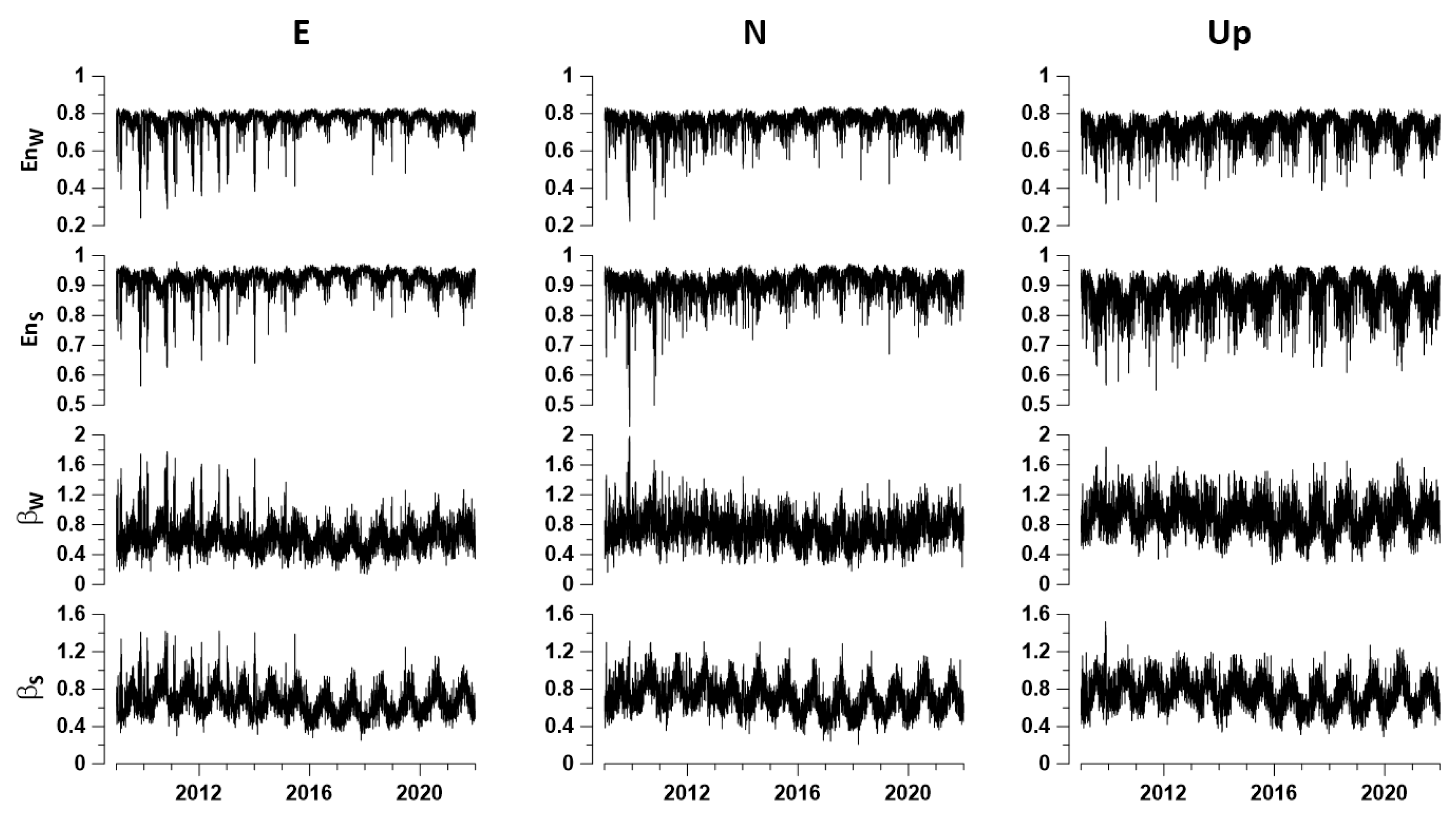
2.1. Minimum Normalized Wavelet-Based Entropy $E{n}_W$ and Wavelet-Based Spectral Index ${\beta }_W$

Let $c_j^{(k)}$ be wavelet coefficients of the analyzed signal $x(t)$, $t=1,\dots ,L$-discrete index numbering successive readings. The upper index $k$ is the number of the detail level of the orthogonal wavelet decomposition, the lower index $j$ numbers the sequence of time interval centers in the vicinity of which the signal convolution with finite elements of the basis is calculated. Below, 17 orthogonal Daubechies wavelets were used: 10 ordinary bases with minimal support with the number of vanishing moments from 1 to 10 and 7 so-called Daubechies symlets [27], with the number of vanishing moments from 4 to 10. For each of the bases, the normalized entropy of the distribution of squares was calculated coefficients and found a basis that provides the minimum entropy:

$$E{n}_W=-{\displaystyle \sum _{k=1}^m{\displaystyle \sum _{j=1}^{M_k}{p}_j^{(k)}\cdot \ln (}}{p}_j^{(k)})/\ln (N_r)\to \min ,\hspace{1em}{p}_j^{(k)}=|c_j^{(k)}{|}^2/{\displaystyle \sum _{l,i}|c_i^{(l)}{|}^2}$$

(1)

Here, $m$ is the number of detail levels taken into consideration, and $M_k$ is the number of wavelet coefficients at the detail level with the number $k$. The number of levels $m$ depends on the length $L$ of the analyzed sample. For example, if $L=2^n$, then $m=n$, and $M_k=2^{(n-k)}$. The condition $L=2^n$ is necessary for applying the fast wavelet transform. If the length $L$ is not equal to a power of two, then the signal $x(t)$ is padded with zeros to the minimum length $N$, which is greater than or equal to $L$: $N=2^n\ge L$. In this case, among the number $2^{(n-k)}$ of all wavelet coefficients at the level $k$, only $L\cdot 2^{-k}$ coefficients correspond to the decomposition of the real signal, while the remaining coefficients are approximately equal to zero due to the addition of zeros to the signal $x(t)$. Thus, in Formula (1) $M_k=L\cdot 2^{-k}$, and only “real” coefficients $c_j^{(k)}$ are used to calculate the entropy. The number $N_r$ in Formula (1) is equal to the number of “real” coefficients, that is $N_r={\displaystyle {\sum }_{k=1}^m{M}_k}$. By construction $0\le E{n}_W\le 1$.

After determining the optimal orthogonal wavelet, we can calculate the average values of the squares of the wavelet coefficients at each detail level:

$$S_k={\displaystyle \sum _{j=1}^{M_k}|c_j^{(k)}{|}^2}/M_k.$$

(2)

The average value (2) of the squares of the wavelet coefficients is the part of the oscillation energy corresponding to the detail level $k$. In other words, this value can be considered as an estimate of the signal $x(t)$ power spectrum in the frequency band corresponding to the detail level $k$ [27]:

$$[f_{\min }^{(k)},f_{\max }^{(k)}]=[1/(2^{(k+1)}\Delta s),1/(2^k\Delta s)]$$

(3)

where $\Delta s$ is the length of the discretization time interval (in our case $\Delta s$ = 5 min). Consider the values of the periods corresponding to the centers of the frequency bands (3):

$$T_k=2/(f_{\min }^{(k)}+f_{\max }^{(k)})=2\Delta s/(2^{-k}+2^{-(k+1)})$$

(4)

Then the quantities $S_k=S(T_k)$, $k=1,\dots ,m$ are similar to the usual Fourier power spectra. The difference lies in the fact that the values (4) are much smoother, which is convenient when calculating the spectral index-the slope of the graph of the logarithm of the power spectrum depending on the logarithm of the period. To calculate the wavelet-based spectral index ${\beta }_W$, consider the following model:

$$\ln (S(T_k))={\beta }_W\cdot \ln (T_k)+c+{\epsilon }_k,\hspace{1em}k=1,\dots ,m$$

(5)

where ${\epsilon }_k$ is a sequence of independent random variables with zero mean. The parameter ${\beta }_W$ in Formula (5) can be called the wavelet-based spectral index, the value of which can be found by the least squares method: ${\displaystyle {\sum }_{k=1}^m{\epsilon }_k^2}\to \underset{c,{\beta }_W}{\min }$.

2.2. Spectral Normalized Entropy $E{n}_S$ and “Usual” Spectral Index ${\beta }_S$

The normalized entropy (1) refers to the entropy of the energy distribution on different time scales (because of the use of finite orthogonal basis functions). At the same time, the entropy can be estimated in the frequency domain. Let $S_{xx}({\omega }_j)$ be an estimate of the signal $x(t)$ power spectrum, ${\omega }_j$ be a sequence of discrete frequency values with a step $\Delta \omega$, ${\omega }_j=(j-1)\cdot \Delta \omega$, $\Delta \omega =2\pi /(N\cdot \Delta s)$, $j=1,\dots ,N$. Quantities

$$p_j^{(S)}=S_{xx}({\omega }_j)/{\displaystyle \sum _{k=1}^{N/2}{S}_{xx}({\omega }_k)},\hspace{1em}j=1,\dots ,N/2,$$

(6)

can be considered as the probabilities of energy distribution in a sequence of non-overlapping frequency intervals of length $\Delta \omega$. Here, $N$ is the minimum length, which is greater than or equal to the sample length $L$: $N=2^n\ge L$, the index $j$ in Formula (6) varies up to $N/2$ due to the symmetry of the power spectrum of real signals with respect to the Nyquist frequency ${\omega }_{N/2+1}$: $S_{xx}({\omega }_{N/2+1-k})=S_{xx}({\omega }_{N/2+1+k})$, $k=1,\dots ,N/2-1$. Similarly to the values (1) and (5), we introduce the spectral normalized entropy $E{n}_S$ and spectral index ${\beta }_S$ according to formulae:

$$\begin{array}{l}E{n}_S=-{\displaystyle \sum _{j=1}^{N/2}{p}_j^{(S)}}\ln (p_j^{(S)})/\ln (N/2),\hspace{1em}0\le E{n}_S\le 1;\\ \ln (S_{xx}(T_j))={\beta }_S\cdot \ln (T_j)+d+{\eta }_j,\hspace{1em}j=1,\dots ,N/2\end{array}$$

(7)

where period $T_j=2\pi /{\omega }_j$, the value of ${\beta }_S$ is defined from the least squares approach: ${\displaystyle {\sum }_{j=1}^{N/2}{\eta }_j^2}\to \underset{d,{\beta }_S}{\min }$, ${\eta }_j$ is a sequence of independent random variables with zero mean.

The values of $E{n}_W$, $E{n}_S$, ${\beta }_W$, and ${\beta }_S$ were estimated in successive time windows consisting of 288 adjacent 5-min readings, which is one day. Before their calculation, the operation of detrending by a polynomial of the fourth order was performed. Thus, for each station, time series were obtained with a time step of 1 day. The maximum entropy method [28] with autoregression order 28 (10% of the sample length in the time window) was used to calculate the power spectrum $S_{xx}({\omega }_j)$ estimate. The proximity of the normalized spectral entropy $E{n}_S$ to the maximum value of 1 means that the energy distribution over frequencies is close to uniform, i.e., the power spectrum is close to the white noise spectrum.

Since displacements of the Earth’s surface in three orthogonal directions are measured at each point of the network, then, when necessary, we will distinguish the values of the analyzed tremor statistics for different directions of surface displacements by the superscript, for example, for entropy (1) $E{n}_W^{(E)}$, $E{n}_W^{(N)}$, $E{n}_W^{(U)}$, where the superscripts correspond to measurements in the E, N, and Up directions. Similar notation will be used for the quantities, $E{n}_S$, ${\beta }_W$, and ${\beta }_S$.

For an auxiliary network of 16 reference points (Figure 1a) 12 time series were determined with a time step of 1 day, the values of which were calculated as medians of the values $(E{n}_W^{(E)},E{n}_W^{(N)},E{n}_W^{(U)})$, $(E{n}_S^{(E)},E{n}_S^{(N)},E{n}_S^{(U)})$, $({\beta }_W^{(E)},{\beta }_W^{(N)},{\beta }_W^{(U)})$, and $({\beta }_S^{(E)},{\beta }_S^{(N)},{\beta }_S^{(U)})$ from the ten nearest operational GPS measurement points. Figure 2 shows graphs of such time series for central reference point number 8. These graphs show a strong seasonal periodicity of tremor properties.

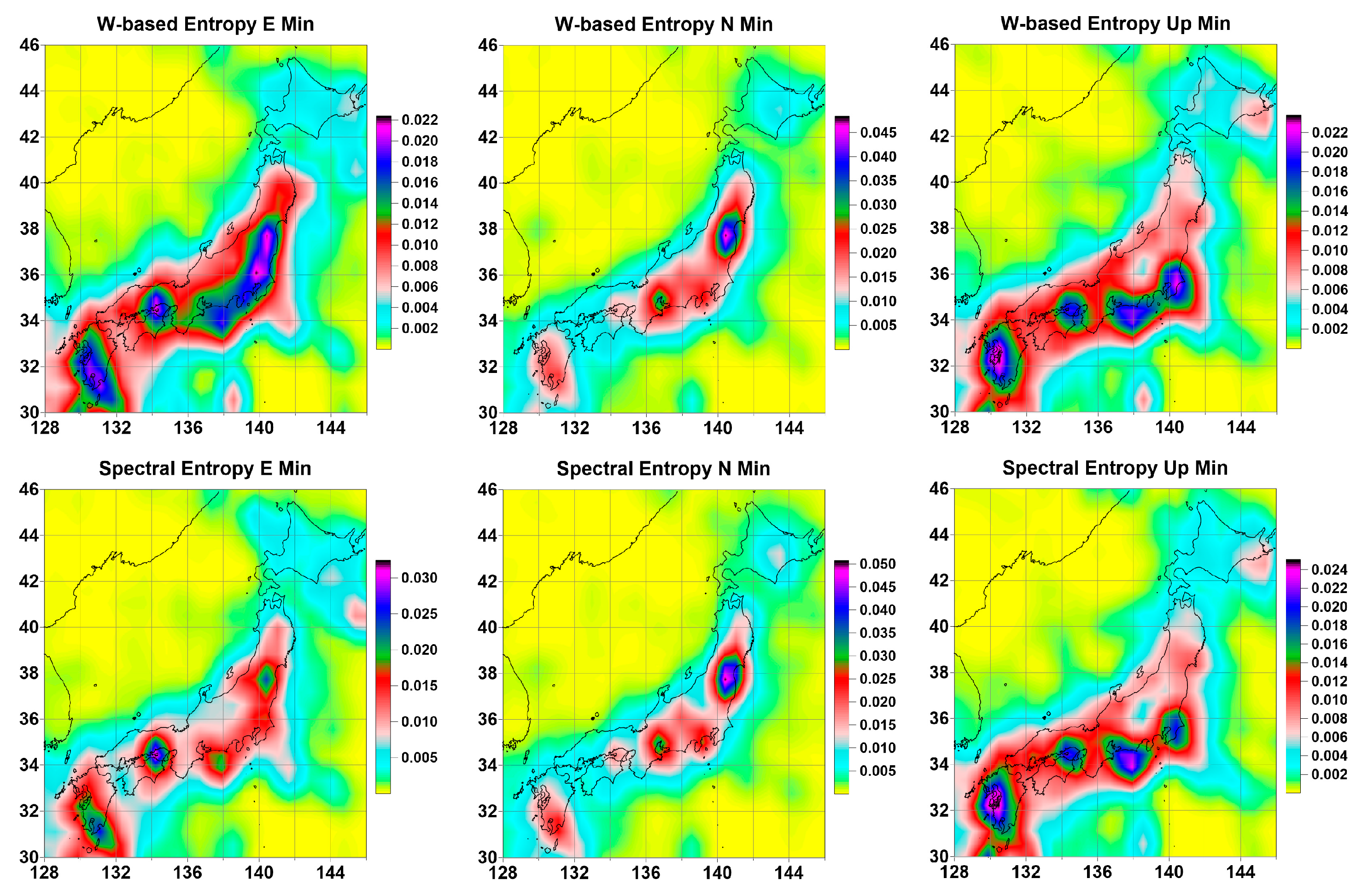
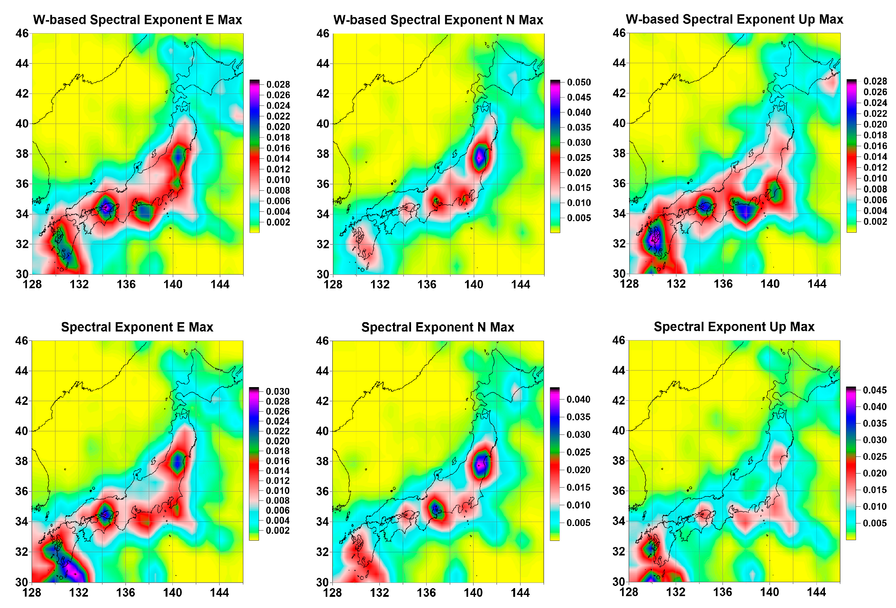
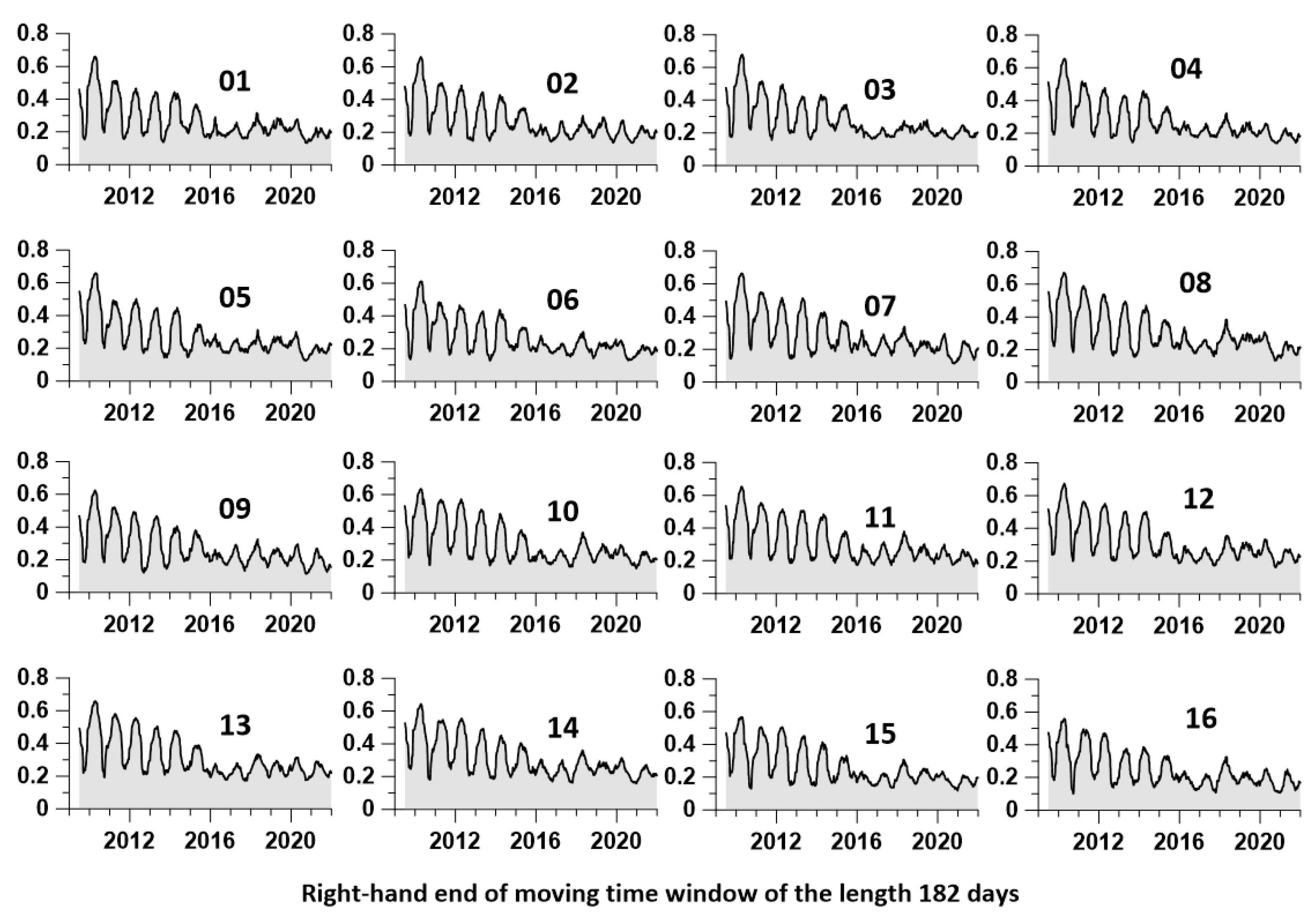
2.3. Probability Densities of Extreme Values

Further, estimates of 12 parameters of the Earth’s surface tremors will be considered in the sequence of time windows 182 days long (half a year), taken with a shift of 3 days. In this case, in each window, we will consider only operable GPS stations, by which we mean those stations for which the total number of missing data in the current window does not exceed 0.1 of the window length.

Consider a regular grid of 30 × 30 nodes covering an area with a latitude from 28° N to 46° N and longitude from 128° E to 146° E. Let $U$ be any value $E{n}_W$, $E{n}_S$, ${\beta }_W$, or ${\beta }_S$, whose estimates are obtained in a sliding time window. For each grid node $(i,j)$ and for each time window labeled $t$ at the right end of the window, find the 10 nearest seismic stations, which gives 10 values of $U$. Let’s take their median value $U_{ij}^{(t)}$.

The values $U_{ij}^{(t)}$ form an “elementary” map corresponding to a time window of 182 days. Consider the values of the parameter as a function of two-dimensional vectors $z_{ij}=(x_i,y_j)$ of longitudes and latitudes of nodes $(i,j)$ in an explicit form: $U_{ij}^{(t)}\equiv U^{(t)}(z_{ij})$. For each “elementary map” with a discrete time index $t$ we find the coordinates of the nodes $z_{mn}^{(t)}=(x_m^{(t)},y_n^{(t)})$ at which the extreme value of $U$ is reached with respect to all other nodes of the regular grid.

If $U=E{n}_W$ or $U=E{n}_S$, then they will look for the minimum values. Otherwise, for $U={\beta }_W$ or $U={\beta }_S$, the maximum values will be searched. As noted above, the choice of a minimum for entropies and a maximum for spectral indexes is due to considerations that anomalous tremor regions should be characterized by the values of statistics that reflect the maximum deviation from the properties of white noise. A cloud of two-dimensional vectors $z_{mn}^{(t)}$ considered within a certain time interval $t\in [t_0,t_1]$ forms a random set. Let us estimate their two-dimensional probability distribution function for each node of the regular grid. For this, the Parzen–Rosenblatt estimate with the Gaussian kernel function [26] will be applied:

$$p(z_{ij}|t_0,t_1)=\frac{1}{2\pi h^2(t_1-t_0+1)}{\displaystyle \sum _{t=t_0}^{t_1}{\displaystyle \sum _{mn}\exp \left(-\frac{|z_{ij}-z_{mn}^{(t)}{|}^2}{2h^2}\right)}}$$

(8)

Here, $h$ is the kernel averaging radius and $t_0,t_1$ are integer indices that enumerate the “elementary” maps of each time window. Thus, $(t_1-t_0+1)$ is the number of time windows in the considered time interval. The width of the smoothing band was used $h={0.5}^{\circ }$ which is approximately equal to 56 km. It should be noticed that the maximum distance from the nearest 10th stations to the reference points equals 47.5 km, the minimum equals 25.4 km, and the median maximum distance equals 37 km.

Figure 3 and Figure 4 show the average distribution maps of the extreme values of the four tremor statistics under consideration for all three displacement components. Even a purely visual perception of these maps suggests that they have a strong similarity to each other. This visual impression is confirmed by the estimate of the matrix of pairwise correlation coefficients presented in

Table 1. Matrix of pairwise correlation coefficients between 12 average probability density maps of extreme values of ground tremor statistics.

	${\mathit{\beta }}_{\mathit{W}}^{(\mathit{E})}$	${\mathit{\beta }}_{\mathit{W}}^{(\mathit{N})}$	${\mathit{\beta }}_{\mathit{W}}^{(\mathit{U})}$	$\mathit{E}{\mathit{n}}_{\mathit{W}}^{(\mathit{E})}$	$\mathit{E}{\mathit{n}}_{\mathit{W}}^{(\mathit{N})}$	$\mathit{E}{\mathit{n}}_{\mathit{W}}^{(\mathit{U})}$	$\mathit{E}{\mathit{n}}_{\mathit{S}}^{(\mathit{E})}$	$\mathit{E}{\mathit{n}}_{\mathit{S}}^{(\mathit{N})}$	$\mathit{E}{\mathit{n}}_{\mathit{S}}^{(\mathit{U})}$	${\mathit{\beta }}_{\mathit{S}}^{(\mathit{E})}$	${\mathit{\beta }}_{\mathit{S}}^{(\mathit{N})}$	${\mathit{\beta }}_{\mathit{S}}^{(\mathit{U})}$
${\mathit{\beta }}_{\mathit{W}}^{(\mathit{E})}$	1	0.8872	0.9315	0.9668	0.8746	0.9269	0.9884	0.8753	0.9336	0.9387	0.9049	0.8469
${\mathit{\beta }}_{\mathit{W}}^{(\mathit{N})}$	0.8872	1	0.7922	0.9052	0.9832	0.8161	0.8799	0.9903	0.8129	0.8215	0.941	0.7044
${\mathit{\beta }}_{\mathit{W}}^{(\mathit{U})}$	0.9315	0.7922	1	0.9129	0.7887	0.9764	0.9193	0.7826	0.9879	0.8994	0.8541	0.8948
$\mathit{E}{\mathit{n}}_{\mathit{W}}^{(\mathit{E})}$	0.9668	0.9052	0.9129	1	0.9141	0.9308	0.9625	0.8975	0.9253	0.9198	0.9045	0.8154
$\mathit{E}{\mathit{n}}_{\mathit{W}}^{(\mathit{N})}$	0.8746	0.9832	0.7887	0.9141	1	0.8227	0.8644	0.9851	0.815	0.8102	0.9372	0.6936
$\mathit{E}{\mathit{n}}_{\mathit{W}}^{(\mathit{U})}$	0.9269	0.8161	0.9764	0.9308	0.8227	1	0.9074	0.8041	0.9894	0.862	0.8402	0.8261
$\mathit{E}{\mathit{n}}_{\mathit{S}}^{(\mathit{E})}$	0.9884	0.8799	0.9193	0.9625	0.8644	0.9074	1	0.8701	0.9127	0.9486	0.8988	0.8565
$\mathit{E}{\mathit{n}}_{\mathit{S}}^{(\mathit{N})}$	0.8753	0.9903	0.7826	0.8975	0.9851	0.8041	0.8701	1	0.803	0.8236	0.9477	0.7055
$\mathit{E}{\mathit{n}}_{\mathit{S}}^{(\mathit{U})}$	0.9336	0.8129	0.9879	0.9253	0.815	0.9894	0.9127	0.803	1	0.8787	0.8524	0.85
${\mathit{\beta }}_{\mathit{S}}^{(\mathit{E})}$	0.9387	0.8215	0.8994	0.9198	0.8102	0.862	0.9486	0.8236	0.8787	1	0.905	0.9326
${\mathit{\beta }}_{\mathit{S}}^{(\mathit{N})}$	0.9049	0.941	0.8541	0.9045	0.9372	0.8402	0.8988	0.9477	0.8524	0.905	1	0.8453
${\mathit{\beta }}_{\mathit{S}}^{(\mathit{U})}$	0.8469	0.7044	0.8948	0.8154	0.6936	0.8261	0.8565	0.7055	0.85	0.9326	0.8453	1

. The minimum value of the correlation coefficient is 0.7044 for the pair, while for the pair the correlation coefficient reaches 0.9903.

The high correlation of probability density maps of the distribution of extreme values of tremor statistics suggests the use of the principal component method [29] to extract the most common distribution over the space of the most common characteristics. To do this, we find the eigenvector of the correlation matrix (Table 1), corresponding to the maximum eigenvalue of this matrix. The squares of the values of the components of this vector (by definition, their sum is equal to 1) will be taken as the weights of digital maps. The result of the weighted average of the probability densities of the distribution of extreme values in Figure 3 and Figure 4 is shown in Figure 5. Figure 5a contains white contour lines which extract regions where the weighted probability density of minimum entropy and maximum spectral index exceeds the level of 98% quantile. These regions are considered as regions of anomalous GPS-measured Earth tremors.

Figure 5b is a plot of the squares of the eigenvector components of the correlation matrix corresponding to the maximum eigenvalue after sorting in descending order. From this plot, it can be seen that the GPS noise statistics corresponding to measurements in the N direction contribute the most to the averaging weights. The smallest contribution corresponds to the vertical Up measurements. However, it should be noted that the differences in the weights are insignificant.

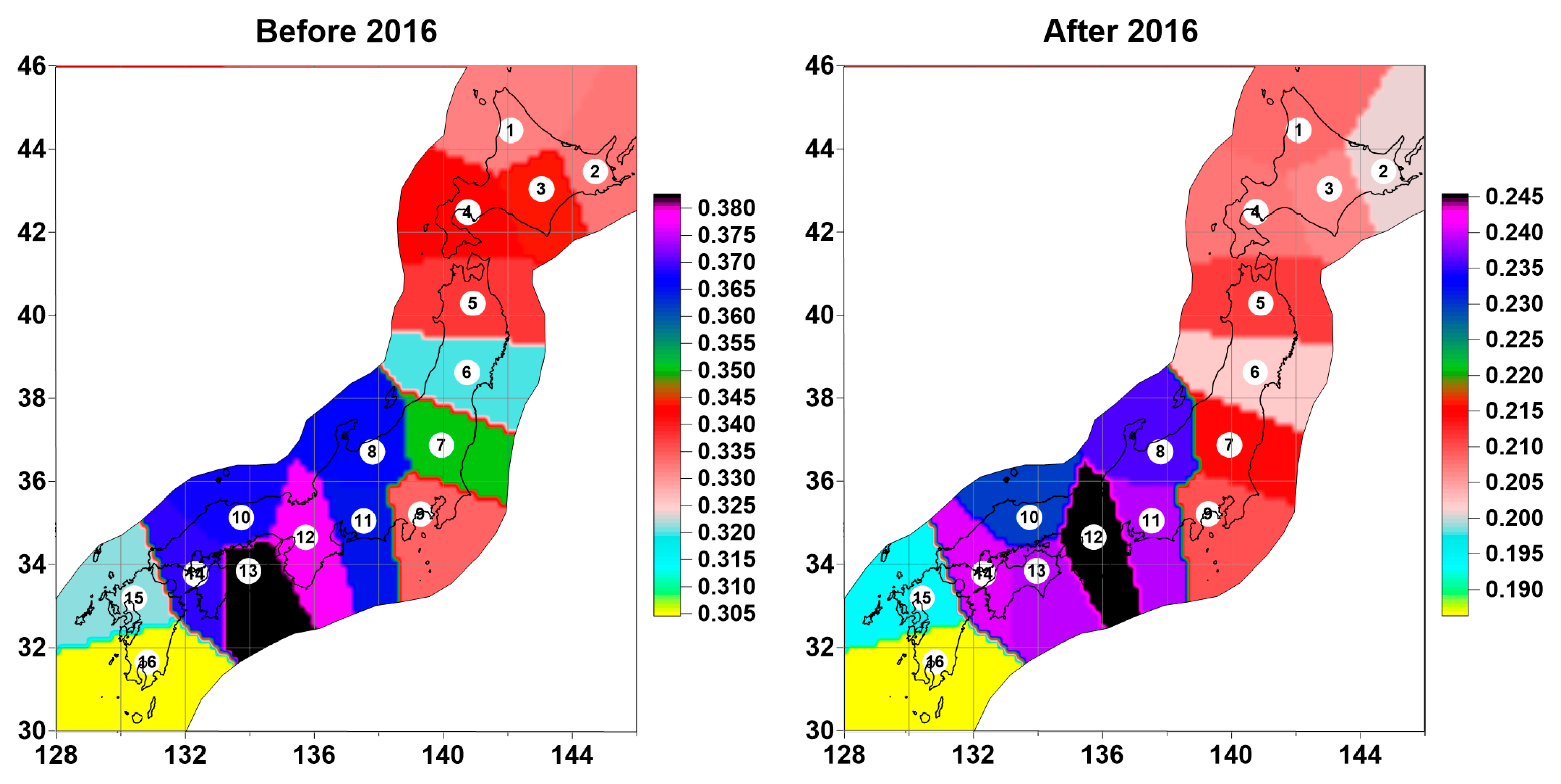
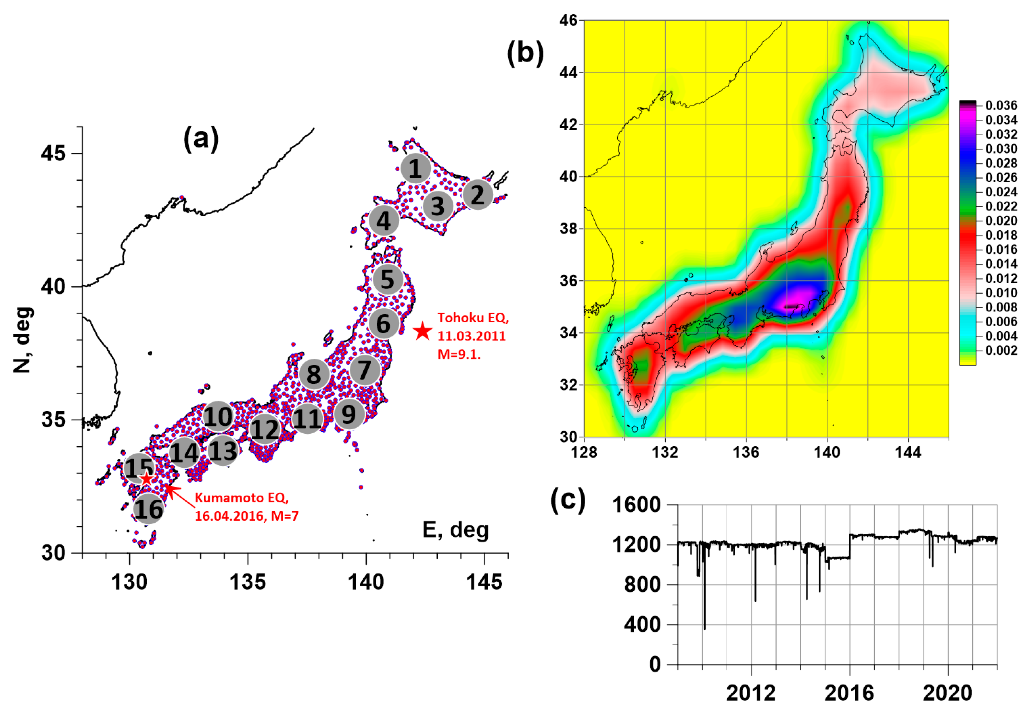
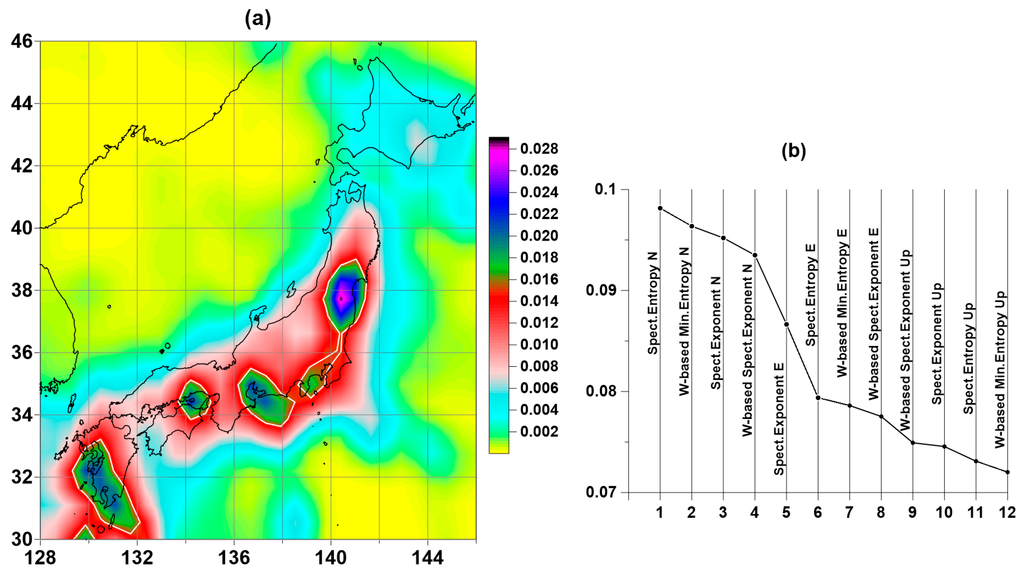
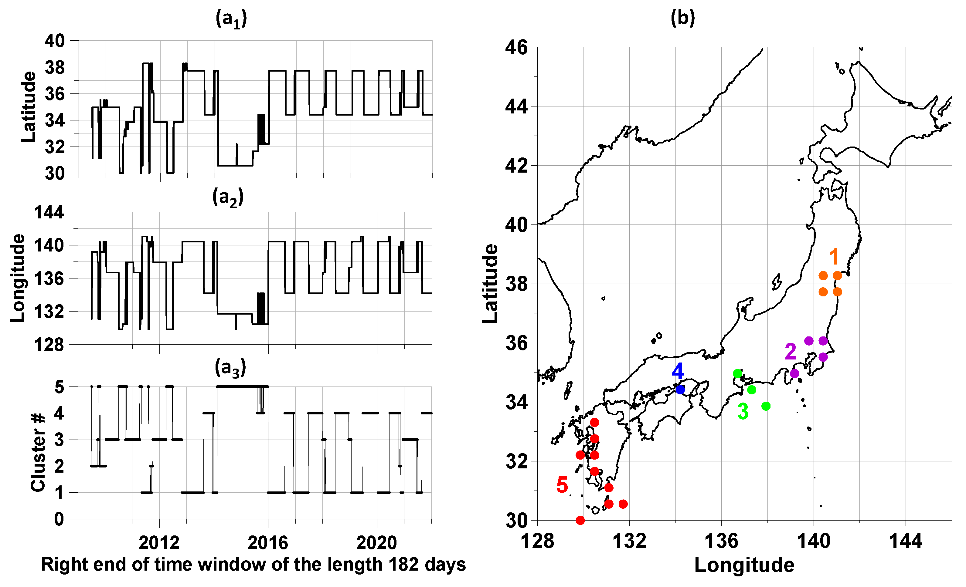
3. Trajectory of Extreme Mean Probability Density Maxima

According to the location of local maxima of the weighted average probability density in Figure 5a, 5 areas of anomalous tremors can be distinguished on the Japanese islands. Since the probability densities were estimated in a sliding time window 182 days long, it is of interest to obtain the trajectory of geographic coordinates corresponding to the position of the local maxima of the averaged probability density in each of the successive time windows.

To obtain such a trajectory for each time window 182 days long, we calculate the weighted average of all 12 probability densities of the distribution of extreme values of the used tremor statistics. Thus, in each time window, we calculate a 12 × 12 correlation matrix similar to the matrix of averaged correlations in Table 1, determine the eigenvector corresponding to the maximum eigenvalue, and use the squares of its components as weights to calculate the average weighted probability density in each window. Next, we find the coordinates of the point that realizes the maximum average density. This sequence of operations performed in each time window makes it possible to obtain the trajectory of geographical coordinates of points that realize the maximum values of the average probability density.

Figure 6(a₁,a₂) shows the graphs of changes in the geographical coordinates of the trajectory points of the maxima of the average weighted probability densities of the extreme values of the tremor statistics. Recall that, according to the construction, these points are nodes of a regular grid of size 30 × 30 covering the region under study. Figure 6b shows the points at which the maxima of the probability densities are realized. These points are divided into five clusters, and cluster number four consists of one point, which is repeatedly visited by the trajectory (plot in Figure 6(a₃)).

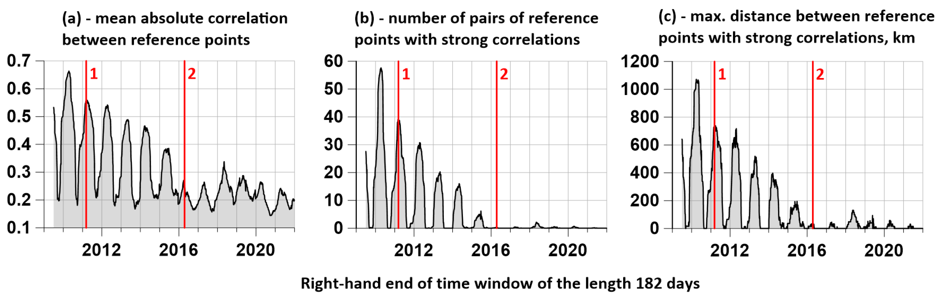
4. Spatial Correlations of Tremor Properties

In this section of the article, spatial correlations between tremor properties in the network of 16 reference points presented in Figure 1 will be investigated. Property values are computed at 16 reference points as medians of daily values from the 10 closest operational stations. Examples of graphs of such time series for reference point #8 are shown in Figure 2.

Consider the correlation coefficients between the same tremor properties at different reference points. Denote by ${\rho }_{ij}^{(\tau )}(P)$ the estimates of the correlation coefficients between the values of the property $P$ at the reference points with numbers $i$ and $j$ for a sequence of time windows 182 days long with time marks $\tau$ of the right ends of the windows. As $P$ can be any of the 12 tremor properties: $E{n}_W^{(E)}$, $E{n}_W^{(N)}$, $E{n}_W^{(U)}$, $E{n}_S^{(E)}$, $E{n}_S^{(N)}$, $E{n}_S^{(U)}$, ${\beta }_W^{(E)}$, ${\beta }_W^{(N)}$, ${\beta }_W^{(U)}$, ${\beta }_S^{(E)}$, ${\beta }_S^{(N)}$, ${\beta }_S^{(U)}$.

For each property, we determine the average value of the correlation coefficients for all pairs of reference points:

$${\overline{\rho }}^{(\tau )}(P)={\displaystyle {\sum }_{(i,j)}{\rho }_{ij}^{(\tau )}(P)}/M$$

(9)

In Formula (9) $M$ is the number of different pairs of reference points. In our case, for 16 reference points $M=120$. Let us denote by $n^{(\tau )}(P)$ the number of pairs of reference points for which the corresponding correlation coefficients ${\rho }_{ij}^{(\tau )}(P)$ exceed the threshold of 0.7 in the time windows with the label of the right end $\tau$. These quantities define some of the strong spatial correlations of tremor properties. The long-range action of strong correlations is described by the values $d^{(\tau )}(P)$ of the maximum distances between those pairs of reference points for which the correlation coefficients ${\rho }_{ij}^{(\tau )}(P)$ exceed the threshold of 0.7.

The obtained values ${\overline{\rho }}^{(\tau )}(P)$, $n^{(\tau )}(P)$, $d^{(\tau )}(P)$ average over all 12 properties, that is, consider the values:

$${\rho }_{\tau }^{*}={\displaystyle \sum _P{\overline{\rho }}^{(\tau )}(P)}/12,\hspace{1em}{n}_{\tau }^{*}={\displaystyle \sum _P{n}^{(\tau )}(P)}/12,\hspace{1em}{d}_{\tau }^{*}={\displaystyle \sum _P{d}^{(\tau )}(P)}/12$$

(10)

Dependences (10) are shown in Figure 7. Quantities (10) could be called measures of the activity of the Earth’s surface tremor.

For each reference point with a number $j=1,\dots ,16$, it is possible to calculate how the average value ${\rho }_{\tau }^{(j)}$ of the correlation coefficients of the tremor statistics with the rest of the reference points changes in each time window. When calculating the values ${\rho }_{\tau }^{(j)}$, the average is made over all 12 properties of the tremor of the Earth’s surface. Graphs of values ${\rho }_{\tau }^{(j)}$ are shown in Figure 8.

The presence of values in 16 reference points distributed throughout Japan allows the construction of maps of spatial values. The construction of such maps provides additional information on the features of the distribution of the correlation of tremor properties. For this, as before when constructing maps in Figure 3 and Figure 4, consider a regular grid of 30 knots in latitude and 30 knots in longitude covering Japan. Then the values at the nodes of the regular grid are calculated by the nearest reference point neighbor method [26]. These values, calculated for each position of the time window at all nodes, make it possible to obtain “elementary” maps of the distribution over the space of average values of the correlation of the tremor property. The result of averaging all “elementary” maps for time windows lying between some 2 dates gives the corresponding averaged map. Figure 9 shows averaged correlation distribution maps for time windows before and after 2016. The distribution of values is given only for the territory of the Japanese Islands covered by the GPS network of stations and some of their surroundings.

It follows from the maps in Figure 9 that the region of the highest spatial correlation of tremor properties is practically unchanged and occupies the southern part of Honshu Island, although the degree of correlation drops noticeably after 2016.

5. Discussion

A new method for estimating the intensity (activity measures) of the Earth’s surface tremor based on measurements by a network of GPS sensors is proposed. The method is based on estimating the trajectory of points corresponding to the maxima of the average weighted probability densities of the distribution of extreme values of tremor statistics in a sliding time window. As tremor statistics, we chose the minimum values of the entropy of the distribution of squared orthogonal wavelet coefficients and the entropy of the power spectrum, as well as the maximum values of the spectral index calculated for the power spectra and the average values of the squared wavelet coefficients. A method has also been developed for estimating the variability of the spatial correlation of tremor properties based on estimates of the correlation values of statistics in an auxiliary network of reference points in a sliding time window.

Methods which used values of spectral index for GPS time series investigations were elaborated in [1,2,3,4,5,6] for identifying models of GPS noise. Similar methods were applied in [21,22,23] for detecting regions which are suspected for increased seismic danger although these methods are based on detrended fluctuations analysis (DFA). However, these methods do not investigate evolution of points providing maximum to probability density of extreme values of spectral index and entropy of GPS noise within moving time window what is the key tool in the current article.

The developed methods were applied to the data of the GPS network in Japan in 2009–2021. Five areas of tremor activity were identified in the center and south of Japan, and a time point (2016) for a significant restructuring of the tremor activation mode was determined. Anomalies of tremor activity were obtained, presumably associated with the preparation of the Tohoku, 11 March 2011, M = 9.1, Lat = 38.32°, Lon = 142.37° and Kumamoto, 16 April 2016, M = 7, Lat = 32.77°, Lon = 130.72° earthquakes.

The trajectory of the points of maximum average probability densities of the distribution of extreme values of tremor statistics and their belonging to the selected 5 activity areas in Figure 6 demonstrates a clear division into two large time fragments with significantly different behaviors; before and after 2016. The interval after 2016 is characterized by stable seasonal periodicity of switching the trajectory of the maxima of the average probability density between the first and fourth clusters. For the first time interval before 2016, we cannot notice such regularity. Thus, it could be called “chaotic,” although this name simply underlines the existence of the change point in the behavior of maxima trajectory. During the two years 2014–2016, tremor activity is concentrated in the south of Japan, in the fifth cluster (Figure 6(a₃)). It is possible that this 2-year concentration of the tremor activation maximum in the fifth cluster reflects the preparation of the Kumamoto earthquake. We also note that the north of Japan in 2009–2021 does not apply to abnormal areas of GPS tremor.

It follows from the graphs in Figure 7 that all average tremor properties are subject to a strong annual periodicity. Note that the maxima of the average correlation ${\rho }_{\tau }^{*}$, the average number $n_{\tau }^{*}$ of pairs of reference points with strong correlations, and the average maximum distances $d_{\tau }^{*}$ of strong correlations correspond to the time windows falling on the winter period and the beginning of spring. Up until 2016, there was a gradual decrease in the annual peaks of the mean values of these measures of tremor activity intensity. After 2016, the average correlations reached a background level of random fluctuations in the vicinity of 0.2, while the values of the measures $n_{\tau }^{*}$ and $d_{\tau }^{*}$ were almost equal to zero. The first half of 2010 displays the maximum value of annual bursts of tremor activity. It is natural to assume that these bursts reflect the process of preparing for the Tohoku mega-earthquake on 11 March 2011.

References

1. Langbein, J.; Johnson, H. Correlated errors in geodetic time series, implications for time-dependent deformation. J. Geophys. Res. 1997, 102, 591–603. [Google Scholar] [CrossRef]
2. Zhang, J.; Bock, Y.; Johnson, H.; Fang, P.; Williams, S.; Genrich, J.; Wdowinski, S.; Behr, J. Southern California permanent GPS geodetic array: Error analysis of daily position estimates and site velocities. J. Geophys. Res. 1997, 102, 18035–18055. [Google Scholar] [CrossRef]
3. Mao, A.; Harrison, C.G.A.; Dixon, T.H. Noise in GPS coordinate time series. J. Geophys. Res. 1999, 104, 2797–2816. [Google Scholar] [CrossRef] [Green Version]
4. Williams, S.D.P.; Bock, Y.; Fang, P.; Jamason, P.; Nikolaidis, R.M.; Prawirodirdjo, L.; Miller, M.; Johnson, D.J. Error analysis of continuous GPS time series. J. Geophys. Res. 2004, 109, B03412. [Google Scholar] [CrossRef] [Green Version]
5. Bos, M.S.; Bastos, L.; Fernandes, R.M.S. The influence of seasonal signals on the estimation of the tectonic motion in short continuous GPS time-series. J. Geodyn. 2010, 49, 205–209. [Google Scholar] [CrossRef] [Green Version]
6. Wang, W.; Zhao, B.; Wang, Q.; Yang, S. Noise analysis of continuous GPS coordinate time series for CMONOC. Adv. Space Res. 2012, 49, 943–956. [Google Scholar] [CrossRef]
7. Caporali, A. Average strain rate in the Italian crust inferred from a permanent GPS network—I. Statistical analysis of the time-series of permanent GPS stations. Geophys. J. Int. 2003, 155, 241–253. [Google Scholar] [CrossRef]
8. Li, J.; Miyashita, K.; Kato, T.; Miyazaki, S. GPS time series modeling by autoregressive moving average method, Application to the crustal deformation in central Japan. Earth Planets Space 2000, 52, 155–162. [Google Scholar] [CrossRef] [Green Version]
9. Beavan, J. Noise properties of continuous GPS data from concrete pillar geodetic monuments in New Zealand and comparison with data from U.S. deep drilled braced monuments. J. Geophys. Res. 2005, 110, B08410. [Google Scholar] [CrossRef]
10. Langbein, J. Noise in GPS displacement measurements from Southern California and Southern Nevada. J. Geophys. Res. 2008, 113, B05405. [Google Scholar] [CrossRef]
11. Blewitt, G.; Lavallee, D. Effects of annual signal on geodetic velocity. J. Geophys. Res. 2002, 107, 2145. [Google Scholar] [CrossRef] [Green Version]
12. Bos, M.S.; Fernandes, R.M.S.; Williams, S.D.P.; Bastos, L. Fast error analysis of continuous GPS observations. J. Geod. 2008, 82, 157–166. [Google Scholar] [CrossRef] [Green Version]
13. Teferle, F.N.; Williams, S.D.P.; Kierulf, H.P.; Bingley, R.M.; Plag, H.P. A continuous GPS coordinate time series analysis strategy for high-accuracy vertical land movements. Phys. Chem. Earth Parts A/B/C 2008, 33, 205–216. [Google Scholar] [CrossRef] [Green Version]
14. Chen, Q.; van Dam, T.; Sneeuw, N.; Collilieux, X.; Weigelt, M.; Rebischung, P. Singular spectrum analysis for modeling seasonal signals from GPS time series. J. Geodyn. 2013, 72, 25–35. [Google Scholar] [CrossRef]
15. Bock, Y.; Melgar, D.; Crowell, B.W. Real-Time Strong-Motion Broadband Displacements from Collocated GPS and Accelerometers. Bull. Seismol. Soc. Am. 2011, 101, 2904–2925. [Google Scholar] [CrossRef]
16. Hackl, M.; Malservisi, R.; Hugentobler, U.; Jiang, Y. Velocity covariance in the presence of anisotropic time correlated noise and transient events in GPS time series. J. Geodyn. 2013, 72, 36–45. [Google Scholar] [CrossRef]
17. Goudarzi, M.A.; Cocard, M.; Santerre, R.; Woldai, T. GPS interactive time series analysis software. GPS Solut. 2013, 17, 595–603. [Google Scholar] [CrossRef]
18. Khelif, S.; Kahlouche, S.; Belbachir, M.F. Analysis of position time series of GPS-DORIS co-located stations. Int. J. Appl. Earth Observ. Geoinf. 2013, 20, 67–76. [Google Scholar] [CrossRef]
19. Lyubushin, A. Global coherence of GPS-measured high-frequency surface tremor motions. GPS Solut. 2018, 22, 116. [Google Scholar] [CrossRef]
20. Lyubushin, A. Field of coherence of GPS-measured earth tremors. GPS Solut. 2019, 23, 120. [Google Scholar] [CrossRef]
21. Filatov, D.M.; Lyubushin, A.A. Fractal analysis of GPS time series for early detection of disastrous seismic events. Phys. A 2017, 469, 718–730. [Google Scholar] [CrossRef]
22. Filatov, D.M.; Lyubushin, A.A. Precursory Analysis of GPS Time Series for Seismic Hazard Assessment. Pure Appl. Geophys. 2019, 177, 509–530. [Google Scholar] [CrossRef]
23. Filatov, D.M.; Lyubushin, A.A. Stochastic dynamical systems always undergo trending mechanisms of transition to criticality. Phys. A 2019, 527, 121309. [Google Scholar] [CrossRef]
24. Nevada Geodetic Laboratory. Available online: http://geodesy.unr.edu/NGLStationPages/RapidStationList (accessed on 1 July 2022).
25. Blewitt, G.; Hammond, W.C.; Kreemer, C. Harnessing the GPS data explosion for interdisciplinary science. Eos 2018, 99, 485. [Google Scholar] [CrossRef]
26. Duda, R.O.; Hart, P.E.; Stork, D.G. Pattern Classification; Wiley: Hoboken, NJ, USA, 2000. [Google Scholar]
27. Mallat, S. A Wavelet Tour of Signal Processing, 2nd ed.; Academic Press: Cambridge, MA, USA, 1999. [Google Scholar]
28. Marple, S.L., Jr. Digital Spectral Analysis with Applications; Prentice-Hall, Inc.: Englewood Cliffs, NJ, USA, 1987. [Google Scholar]
29. Jolliffe, I.T. Principal Component Analysis; Springer: Berlin/Heidelberg, Germany, 1986. [Google Scholar]
Figure 1. (a)—position of GPS measurement points in Japan (purple dots) and positions of 16 reference points (grey circles), red stars indicate epicenters of Tohoku (11 March 2011, M = 9.1) and Kumamoto (16 April 2016, M = 7) earthquakes; (b)—density of GPS stations; (c)—daily numbers of operational GPS stations in Japan, 2009–2021.
Applsci 12 07297 g001
Figure 2. Plots of daily values for four GPS ground tremor properties for reference point number 8 for three ground displacement components E, N, and Up. The property values are calculated as medians from the ten nearest operable stations.
Applsci 12 07297 g002
Figure 3. Averaged maps of the distribution of the minimum values of the wavelet-based and spectral entropies of the GPS tremor for the displacement components E, N, and Up on a regular grid of 30 × 30 nodes.
Applsci 12 07297 g003
Figure 4. Averaged maps of the distribution of the maximum values of the wavelet-based and usual spectral indices of the GPS tremor for the displacement components E, N, and Up on a regular grid of 30 × 30 nodes.
Applsci 12 07297 g004
Figure 5. (a)—weighted average map of distribution of extreme values of four properties of the Earth’s surface tremors for three displacement components E, N, and Up, white contour lines extract anomalous regions of Earth’s tremor as 98% quantile of probability density values; (b)—values of the squares of the main eigenvector components of the correlation matrix between the distribution maps of extreme values of four daily tremor properties of the Earth’s surface for three displacement components E, N, and Up on a regular 30 × 30 grid of nodes, sorted in descending order.
Applsci 12 07297 g005
Figure 6. (a1,a2) are the latitudes and longitudes of the nodes of a regular grid of 30 × 30 in size, in which the maxima of the average weighted probability density of the distribution of extreme values of the properties of the tremor of the Earth’s surface were realized in sliding time windows 182 days long; (a3) are the corresponding numbers of clusters of maximum points. (b)—division of points of the trajectory of maxima into five clusters.
Applsci 12 07297 g006
Figure 7. (a) is a plot of mean correlations ρ τ * ; (b) is a graph of the average number n τ * of pairs of control points for which the correlations exceeded the threshold of 0.7; (c) is a graph of the average maximum distances d τ * between those pairs of control points for which the correlation coefficients exceed the threshold of 0.7. Vertical red lines indicate time moments of earthquakes: 1—Tohoku, 11 March 2011, M = 9.1; 2—Kumamoto, 16 April 2016, M = 7.
Applsci 12 07297 g007
Figure 8. Graphs of average correlation coefficients ρ τ ( j ) for each reference point with all other reference points.
Applsci 12 07297 g008
Figure 9. Average maps of interpolation of the distribution of average correlations ρ τ ( j ) from reference points for time windows before and after 2016, obtained by the nearest neighbor method. The numbered white circles represent the positions of the 16 reference points.
Applsci 12 07297 g009