Evaluation of Internal Cracks in Turbine Blade Thermal Barrier Coating Using Enhanced Multi-Scale Faster R-CNN Model

Abstract

Thermal Barrier Coatings (TBCs) have good performance in heat insulation during service on turbine blades. However, the accumulated residual stress will form cracks, which can easily lead to coating failure. To ensure safe operation, it is necessary to find a method that can evaluate the health of the coating. In this paper, a non-destructive evaluation technique based on Multi-Scale Enhanced-Faster R-CNN (MSE-Faster R-CNN) is proposed. Firstly, the Visual Geometry Group Network19 layer (VGG-19) was adopted as the baseline network to find the candidate crack Region of Interest (ROI). Considering the influence of the crack on the surroundings, the ROI was expanded to obtain the context information. Secondly, a multi-scale Faster R-CNN detector was used to refine the candidate regions, and provided a comprehensive feature for better crack detection. Finally, a fusion lifetime prediction model was proposed to estimate the remaining lifetime of the TBC. Extensive experiments were conducted to evaluate the performance of the proposed method. The results demonstrated that the proposed method can accurately locate (0.898) and detect (0.806) the cracks in different scales, and the lifetime estimation result reached the best level (Root Mean Square Error (RMSE) = 2.7); there wasas also an acceptable time cost (1.63 s), and all detection conditions of the error rates were below 15%, achieving the best results among the state-of-art methods.

1. Introduction

The working temperature of a gas turbine is rising continuously due to the continuous pursuit of performance. A common way to deal with this situation is to spray Thermal Barrier Coatings (TBCs) on the turbine blades, so that the components can bear a large temperature gradient when exposed to heat flow [1,2]. During long term service, cracks are one of the most common and serious defects in TBCs [3]. Since TBC is a multilayer structure including top-coating layer, transition layer and the substrate, under high temperature and harsh working conditions, the thermodynamic performance of different layers become inconsistent, especially though a mismatch of thermal expansion coefficients. Such mismatch between the layers will induce residual stress, which is considered to be the major cause of the cracks [4]. The thermal insulation performance of the TBC will significantly be reduced by a large sized crack or the penetration crack. When growing to a certain extent, a crack will cause the coating to reach spallation, which makes TBC totally fail and thus creates serious security problems. Therefore, implementing TBC crack detection is of great importance.

The main crack detection methods include manual detection, ultrasonic detection, laser scanning detection, infrared image-based detection, etc. [5]. Traditional manual detection requires professional staff to shut down the gas turbine regularly and observe whether the TBCs have cracks. This approach has many disadvantages such as being expensive, subjective, and inefficient. Alternatives such as ultrasonic detection, laser scanning detection and infrared image-based detection are regarded as non-destructive evaluation methods [6,7]. However, due to the limitations of the working environment, ultrasonic and laser detection is difficult to use for on-line monitoring. In contrast, infrared image detection has relatively low requirements for the working environment [8,9]. In the neighborhood of 1500 °C, the infrared thermal imager only needs a heat shield to run successfully. Hence, studies of infrared detection technology have garnered increasing attention [10,11,12,13].

Infrared image processing methods for detection of coating defects usually have four steps: image pre-procession, image segmentation, feature extraction, and classifier construction [14]. Image pre-procession methods are mostly for improving image quality by image de-noising and enhancement [15,16]. Image segmentation methods collect information and characteristics from the image, and divide the image into Regions of Interest (ROIs) and background. Researchers usually start ROIs extraction by either applying a kind of designated threshold, or edge detection by analyzing the local gradients [17,18]. Feature extraction and classification methods of images are also extensively studied [19,20,21,22]. However, traditional image processing methods are used for surface cracks detection. It is generally agreed that stress accumulation during service will form several micro-cracks at the interface, and then expand to form a dominant interface crack, which may grow vertically to the surface and eventually cause spallation [4,23]. In addition, the growth of thermally grown oxide will also bring residual stress, resulting in horizontal cracks and spallation in the coating [24,25]. Therefore, it is possible to have both surface cracks and internal cracks in the TBCs. However, the characteristics of surface cracks and internal cracks are very different. Surface cracks generally have a certain linear feature while the features of internal cracks are very fuzzy. Moreover, there are plenty of pores in the coating. The size and shape of a small internal crack is so close to the pore, that it will show a very similar effect on the temperature distribution. Such pores will bring many false alarm points in internal crack detection and thus make traditional image processing methods less accurate.

Due to the limitations of traditional image processing methods and the advantages of the powerful decoupling feature extraction ability of deep learning, methods based on deep learning are considered a promising solution to this problem. Recently, various deep learning models, such as Convolutional Neural Network (CNN), Region-CNN (R-CNN), Faster R-CNN and You Only Look Once (YOLO) [26,27,28,29], have received much attention. Effective feature representation and recognition can be obtained through these deep learning methods by automatic learning, and the process of using complex feature extraction algorithms as well as crack identification are eliminated. However, these deep learning methods often have high requirements for the quantity and quality of training data. CNN and R-CNN will generate a large number of candidate regions when selecting candidate regions, which will seriously increase the data. In reality, collecting a large number of labeled coating crack datasets is time-consuming, and to our knowledge, there is no public available dataset on internal cracks in the coating. Transfer learning can transfer the network weight trained from other similar datasets to the target network, which can train the parameters faster and better without having to train from scratch, and can solve the problem of lack of data to a certain extent. Compared with YOLO, the Region Proposal Network (RPN) structure of Faster R-CNN can make the positive and negative samples more balanced, so as to obtain a abetter training effect. YOLO uses a one-stage detector, which mixes the work of positioning and classification. There are no special parameters for candidate regions which would make the training more difficult. The two-stage detector of Faster R-CNN can avoid this problem, thus increasing the training and testing accuracy.

For the above reasons, in this paper, an internal crack detection scheme based on Multi Scale Enhanced-Faster R-CNN (MSE-Faster R-CNN) is proposed. Visual Geometry Group Network (VGG-19) was adopted as the baseline network to find the candidate crack Region of Interest (ROI). Then, the ROI was expanded to obtain the context information. Through a multi-scale Faster R-CNN detector, the state of the candidate region can be determined.

This manuscript summarizes the results in the following way. Firstly, the architecture and principle of MSE-Faster R-CNN is presented. Secondly, the dataset preparation and augmentation, as well as the experimental settings are introduced. Thirdly, the performance of MSE-Faster R-CNN in different crack scales is tested and discussed as well as compared to other state-of-art methods. Finally, an information entropy fusion lifetime estimation model is applied using the crack detection experimental results.

2. Principle of the Crack Detection and Lifetime Prediction Model

2.1. Architecture of MSE-Faster R-CNN

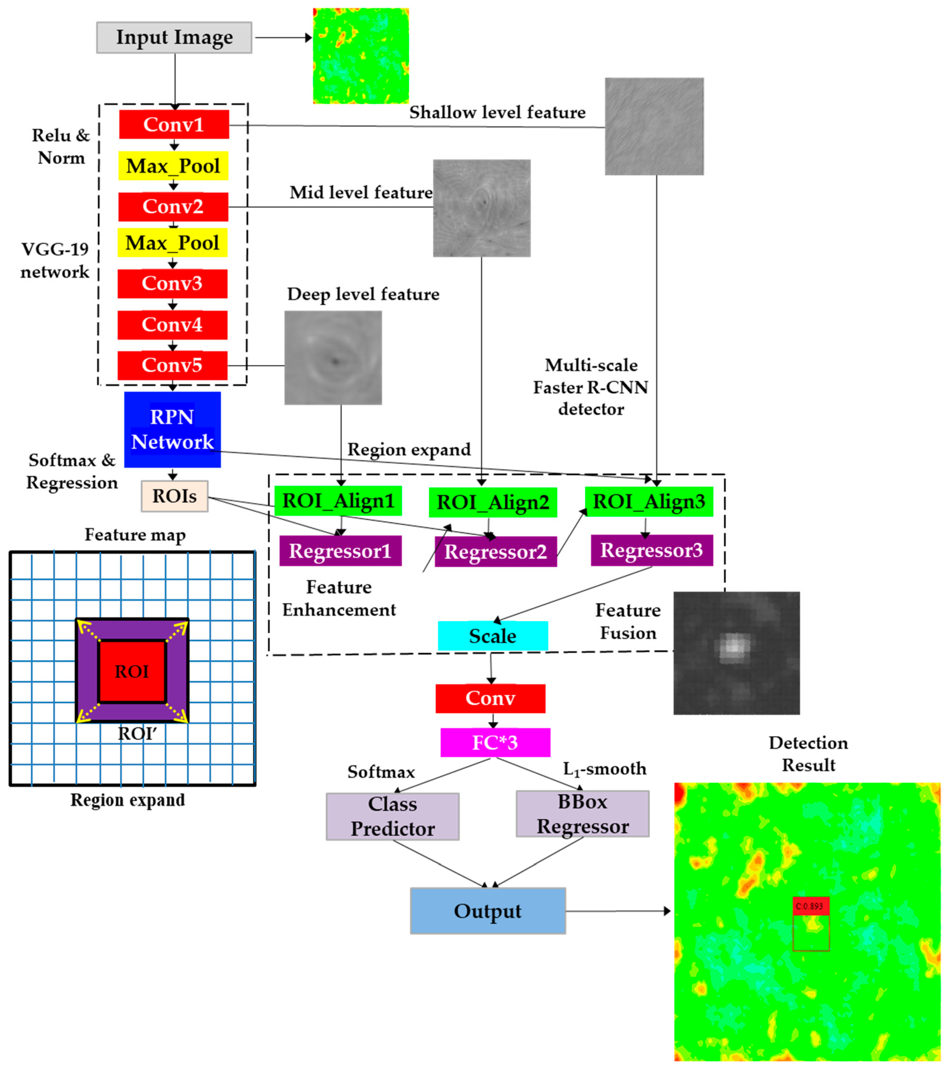
Figure 1 depicts the overall structure of MSE-Faster R-CNN. The MSE-Faster R-CNN consists of two modules: the Regional Proposal Network (RPN) and the Multi-scale Fast R-CNN detector (see Figure 1). RPN is a fully convolutional network for efficiently generating region proposals with a wide range of scales and aspect ratios. Region proposals are rectangular regions which contain candidate cracks. MSE-Faster R-CNN detector is used to refine the proposals. The RPN and the MSE-Faster R-CNN detector share the same convolutional layers, allowing for joint training. The MSE-Faster R-CNN runs through the CNN only once for the entire input image and then refines crack proposals. Due to the sharing of convolutional layers, it is possible to use a deep CNN network for generating high quality crack proposals. As a small size structure, the crack can easily lose detail in the process of feature extraction. Considering that the detailed information of the low-level convolution output is more abundant than that of the high-level convolution output, VGG-19 [30] is selected as the pre-training network, and three segments of convolution layers are selected and max-pooled to obtain feature maps of different scales.

Figure 1 shows the flow of internal crack detection using MSE-Faster R-CNN. The input image is firstly sent to the vgg-19 network for feature extraction. Different scales of feature maps are obtained after convolution, max-pooling and Relu activation layer. These feature maps are then input into the RPN network. Several ROIs, which are rectangular anchor frames selected by NMS that may be crack areas, will be obtained. Considering that the crack will have a significant temperature effect on the surrounding area, the ROIs regions are expanded in this paper, as Figure 1 shows. By fusing the expanded feature maps with different scales, the feature expression ability of the network can be strengthened. This enhanced and fused feature map will be input to the convolution layer and the three fully connected layers. The final crack diagnosis result and anchor frame position will be obtained through softmax classification and L₁-smooth regression discriminant function.

However, since the crack has characteristics of various shapes and sizes, when the input image scale is large, the resolution of the feature image becomes smaller after multiple down-sampling. Although the ROI becomes larger, the detailed features will be lost, and the utilization of semantic information obtained by multi-scale receptive field is low. To solve the above problem, this paper enhances the fusion of multi-scale feature images. The high-dimensional convolution features are refined and input into the low-dimensional feature map. Then the features are fused to avoid misleading the positioning and recognition tasks caused by a large number of complex context relations. Thus, the useful information around the object is significantly enhanced. In this way, the structure can integrate the features of receptive fields from different sizes, increase the receptive field and make full use of the contextual semantic information of the object, thus improving the sensitivity to the internal cracks in the coating.

2.2. Operation of MSE-Faster R-CNN Crack Detector

The MSE-Faster R-CNN detector takes multiple ROIs as input. For each ROI (see Figure 1), a fixed-length feature vector is extracted by the ROIs pooling layer from the convolutional layer. The final feature vector is fed into a sequence of fully connected (FC) layers. The outputs of the detector through the Softmax layer and the bounding-box regressor layer include (1) Softmax probabilities which estimate over the crack class and the background class and (2) the crack bounding-box.

As many bounding-boxes overlap highly with each other, non-maximum suppression (NMS) is applied to merge bounding-boxes that have high Intersection-over-Union (IoU). After NMS, the remaining bounding-box is ranked based on the crack probability score, and only the top oneis used for detection.

For training RPNs, each proposal is assigned a binary class label which indicates whether the proposal is a crack or just background. A positive training example is designated if the proposal overlaps with a ground-truth box with an IoU more than a predefined threshold (0.7), or if it has the highest IoU with a ground-truth. A proposal will be assigned as a negative example if its maximum IoU is lower than the predefined threshold (0.3) for all ground-truth boxes.

Following the multitask loss in Faster R-CNN network, the RPN is trained by a multitask loss, which is defined as [28]:

$$L\left(\right\{p_i\},\{t_i\left\}\right)=\frac{1}{N_{cls}}{\displaystyle \sum }_i{L}_{cls}\left(p_i,p_i{}^{*}\right)+\mathsf{\lambda }\frac{1}{N_{reg}}{\displaystyle \sum }_i{p}_i{}^{*}{L}_{reg}\left(t_i,t_i{}^{*}\right)$$

(1)

where i is the index of an anchor. The multi-task loss has two parts, a classification component cls and a regression component reg. In Equation (1), p_i is the predicted probability of the anchor being a crack while p_i^* is the true category of the anchor. The ground-truth label is 1 if the anchor is positive and 0 if the anchor is negative. t_i is a vector representing the 4 parameterized coordinates of the predicted bounding-box; and t_i^* is the vector of the ground-truth box associated with a positive anchor. The classification loss L_cls is normalized by N_cls and the regression loss L_reg is normalized and weighted by a balancing parameter λ. In this paper, considering a large number of small pores in the coating model, λ is set to 6. Such a balancing parameter setting will increase the influence of diagnostic error, so as to minimize the influence of pores. The N_cls term in (1) is normalized by the mini-batch size. Bounding-box regression aims to find the best nearby ground-truth box of an anchor box. The parameterization of the 4 coordinates of an anchor is described as follows [27]:

$$\{\begin{array}{c}{t}_x=\frac{\left(\mathrm{x}-x_a\right)}{w_a}\\ \begin{array}{l}{t}_y=\frac{(y-y_a)}{w_a}\\ t_w=\log \frac{w}{w_a}\\ t_h=\log \frac{h}{h_a}\end{array}\end{array}$$

(2)

$$\{\begin{array}{c}{t}_x*=\frac{(x*-x_a)}{w_a}\\ \begin{array}{l}{t}_y*=\frac{(y*-y_a)}{w_a}\\ t_w*=\log \frac{w*}{w_a*}\\ t_h*=\log \frac{h*}{h_a*}\end{array}\end{array}$$

(3)

where x, y, w, and h denote the bounding-box’s center coordinates, width, and depth, respectively. x, x_a and x_a* are for the predicted box, anchor box and ground-truth box, respectively. Similar definitions are also applied for y, w and h.

The bounding-box regression is achieved by using features with the same spatial size on the feature maps. A set of bounding-box regressors is trained to adapt for varying size of cracks. The adjusted bounding-box scale is more suitable for crack detection.

VGG-19 is used for generating candidate crack regions for the RPN. It is pre-trained in the ImageNet Dataset. Since the RPN and MSE-Faster R-CNN detector can share the same convolutional layers, these two networks can be trained jointly to learn a unified network through the following 4-step process: first, training the RPN; second, training the detector network using proposals generated by the trained RPN; third, initializing RPN training by the detector network but only training the specific layers; and finally, training the detector network using the new RPN’s proposals.

2.3. Fusion Lifetime Prediction Model

Reference [31] established a lifetime prediction model of coatings corresponding to crack length based on the assumption that interfacial oxidation is the major factor controlling the lifetime of coatings. In service, the residual stress in the ceramic layer increases with the number of thermal cycles. The accumulation of residual stress caused by oxidation promotes the length of cracks in the coating, and finally leads to the failure of the coating.

In the real operation of a gas turbine, there are many sources of uncertainty in residual lifetime prediction, such as measurement error, randomness of load, change of working conditions, etc., so it is necessary to quantify and manage these uncertainties. Relevance Vector Machine (RVM) based on sparse Bayesian learning is a very suitable algorithm for residual lifetime prediction. It retains the idea of kernel mapping of the Support Vector Machine (SVM) and adopts some strategies to reduce the number of correlation vectors compared with SVM, which greatly reduces the prediction time while ensuring the prediction accuracy. Moreover, compared with traditional neural network and SVM, RVM can obtain probability output and better represent the uncertainty of residual lifetime prediction, so this paper uses RVM as one of the residual lifetime prediction methods.

The steps of RVM are as follows:

• Input vector set (porosity, crack length, location, coating temperature) and target vector set (remaining useful lifetime RUL) are respectively formed for the data of each input image;
• The radial basis function (RBF) was used as the kernel function, and the parameter of RBF was optimized by the five-fold cross validation method, with the objective of minimum mean square error;
• RVM regression model was established by using the optimal parameter on each input image, and the optimal remaining lifetime value of the current image was obtained by prediction.
• The average value of the remaining lifetime in a period of time was counted and the RUL value of the transition fragment was replaced by the mean value;

The training of RVM can be completed by repeating 2–4 until it stops meeting certain convergence criteria, that is, when the change of mean square error is within the pre-set threshold.

Due to the complex relationship between condition monitoring data and remaining lifetime, it is difficult to determine which prediction method will perform better in a specific situation. Therefore, a feasible way to fuse the lifetime prediction results under different conditions is to fuse multiple methods. Compared with a single prediction method, the fusion of multiple prediction methods can effectively improve the accuracy and robustness of prediction.

In this paper, a RUL prediction fusion method based on information entropy is proposed, and the RUL prediction results using evidence theory regression, support vector machine and neural network are fused according to this method. The basic principle of the fusion method based on information entropy is that for each prediction method member, if the variability of the prediction error sequence is large, its corresponding weight should be set relatively small during synthesis. The specific calculation process is as follows [31].

$$e_{mt}=\{\begin{array}{c}1,\left|\frac{{rul}_t-{rul}_{mt}}{{rul}_t}\right|\ge 1;\\ \left|\frac{{rul}_t-{rul}_{mt}}{{rul}_t}\right|,\left|\frac{{rul}_t-{rul}_{rt}}{{rul}_t}\right|<1\end{array}$$

(4)

In Equation (4), rul_t represents the ground truth RUL value of TBC at time t, rul_mt represents the RUL value of TBC estimated by the physical model, and rul_rt is the RUL value of TBC estimated by RVM model. For each prediction method, calculate the prediction relative error (e_mt) at all N monitoring points, obtain the sequence composed of relative error, and normalize it, to obtain p_mt:

$$p_{mt}=\frac{e_{mt}}{{{\displaystyle \sum }}_{t=1}^N{e}_{mt}},t=1,2,\cdots ,N$$

(5)

Then, the information entropy of the relative error sequence of the physical model prediction method, h_m is calculated as follows:

$$h_m=-k_h{\displaystyle \sum }_{t=1}^N{p}_{mt}{lnp}_{mt}$$

(6)

where k_h is a constant greater than 0 and h_m ≥ 0. Then, the coefficient of variation of the prediction method d_m is calculated. Since 0 ≤ d_m ≤ 1, according to the principle that the information entropy of the prediction relative error sequence is opposite to the variability, the variability coefficient d_m can be denoted as:

$$d_m=1-h_m$$

(7)

Finally, the weight of the physical model prediction method w_m can be calculated by the following equation:

$$w_m=\left(1-\frac{d_m}{d_m+d_r}\right)$$

(8)

Similarly, the parameters of the lifetime prediction method of RVM (e_rt, p_rt, h_r, d_r and w_r) can also be calculated. The final lifetime prediction result can be obtained by weighted sum of the predicted results [32]:

$$RUL=w_m{rul}_m+w_r{rul}_r$$

(9)

3. Data Preparation and Experiments Setup

3.1. Dataset Description

It is extremely difficult to produce different geometrical parameters of internal cracks using a large number of real coating samples. The coating samples obtained by real experiments often have low precision, low efficiency and high cost. The reason is that in the real experiment, the internal cracks should be added in the coating manufacturing stage. Once the internal cracks are generated in the coating, it is difficult to modify the parameters of the crack. Therefore, a large number of workpieces are needed to generate cracks of different lengths or positions. In addition, it is difficult to control the crack parameters accurately in the real experiment since the procedure is inside the coating. If a numerical TBC and crack model can be established, it will be very convenient to test and develop the performance of the crack detection scheme. Reference [32] developed a 3D finite element heat transfer model to evaluate surface crack depth using lock-in infrared thermography. Similarly, in this paper, microstructure reconstruction software was developed by our team to establish the TBC model [33,34] with a variety of sizes and locations of internal cracks (see Appendix A). The material of the TBC is 8% mol yttria-doped zirconia (8YSZ). Nickel base alloy is used as substrate material. There is a 10 μm thick bonding layer over the substrate, which is composed of thermally grown oxides (TGO).

Table 1. Calculation parameters of the numerical model.

Parameter	Value
Air thermal conductivity/W·m−1 °C−1	0.0807
8YSZ thermal conductivity/W·m−1 °C−1	2.43
Topcoat temperature/°C	1212
Substrate temperature/°C	844
Horizontal velocity of upper boundary fluid/m·s−1	23

lists the calculation parameters of the model. The initial thermal excitation comes from the air temperature at the top of the coating and the substrate temperature. By applying the calculation parameters, calculation boundaries, flow and thermal boundaries as well as the evolution equation of the temperature fields given in reference [35], the steady-state temperature distributions of the TBC can be then calculated. It should be noted that the numerical coating model is based on the assumption that the pore distribution of the coating remains unchanged in a period of time (This is normal in reality, since the pore location of the coating are determined at the time of manufacture. Only in some cases, such as corrosion, can this characteristic be changed). The dataset contains 245 infrared images of TBCs with resolution of 360 × 360 pixels and 116 images with resolution of 720 × 300. The porosity is set from 1% to 25% (step size = 1%) [36]. The crack width is set at 4 μm and 12 μm and the crack length is set from 10 μm to 260 μm (the crack with a width of 4 μm cannot be set longer than 80 μm). Ellipsoid cracks are selected as the morphology and the locations of cracks are set randomly.

3.2. Dataset Augmentation and Experimental Setup

Deep learning target detection always needs a large number of images to prevent model over-fitting. Since there is no public infrared image data set of high-temperature TBCs, and the simulation samples are relatively limited, a series of operations were carried out to expand the dataset. The size of the dataset can be augmented through certain geometric transformations and size transformations of the image, such as rotation, flip, clipping, scaling transformation, and so on. Clipping did not work well since the method of crop and mix often does not meet the characteristics of coating heat conduction, and will make the infrared image very unnatural. Although the scale of coating cracks may change, the pores of the coating are often fixed, so changing the scale to enhance the data is also ineffective. Rotation and flip are adopted and proved useful in this paper. The original image dataset is enhanced to 1083 images. In order to make full use of the dataset, a 5-fold cross validation is conducted. The specific steps are as follows: the initial sampling is divided into 5 sub samples, a single sub sample is retained as the data of the validation model, and the other 4 samples are used for training. The cross validation is repeated 5 times, and each sub sample is verified once. The results of 5 times in total are used to obtain the estimation result.

The code is implemented in the TensorFlow framework. TensorFlow is an end to end software library developed by the Google brain team for machine learning. It contains various open source tools and libraries, enabling developers to build and deploy applications supported by deep learning. Adaptive momentum (ADAM) is chosen as the optimizer. Adam is an adaptive moment estimation gradient descent algorithm. Its super parameters are well interpretable, and can generate adaptive learning rates for different network parameters, so that the gradient update is more stable and natural, and efficient convergence can be achieved. The mini-batch size of the RPN stage and classification stage is 8. The initial learning rate of the first 35,000 iterations is 0.0001 while the learning rate of the subsequent 5000 iterations is 0.001 to increase the training speed. The maximum iterations are set to 40,000. The momentum is 0.9 and the weight decay is 0.0001.

In the stage of RPN, various shape and scale parameters of anchors are set, as well as the thresholds of anchors and true cracks to select positive and negative samples. In training the RPN network, when the overlap between the ground truth and the anchors meets the conditions, the anchors can be used to train the RPN network. Figure 2 shows the training curve of the MSE-Faster R-CNN. In this figure, Loss_cls represents the loss of classification, which refers to the difference between the predicted class and the actual class through the Softmax layer. Loss_bbox represents the loss of crack location, which refers to the difference between the predicted anchor location and the actual anchor location during the training stage by calculating the most fit anchor box after NMS. In the training phase, these two loss functions are minimized to achieve higher accuracy. From the figure it can be seen that both the loss of classification and the loss of regression converge after 40,000 iterations, decreasing from 90% of the initial iteration to less than 15%.

4. Experiments Results and Discussions

4.1. Evaluation Criteria

In this paper, the performance of crack detection is evaluated by calculating the detection accuracy (D_a). It is calculated by Precision and Recall. The equations are:

$$Precision=\frac{TP}{TP+FP}$$

(10)

$$Recall=\frac{TP}{TP+FN}$$

(11)

$$D_a=(1+k)\cdot \frac{Precision\cdot Recall}{k Precision+Recall}$$

(12)

In Equations (10) and (11), TP, FP, and FN are the proportions of crack detection that are considered true positives, false positives, and false negatives, respectively. In Equation (12), it can be seen that k controls the weight of Precision and Recall. When k is set as a high value, it indicates that Precision is more important in diagnostic performance, and vice versa. Here k is set as 1 to indicate that the Precision and Recall are looked as of equivalent importance.

Another measure to evaluate the performance of the algorithm is the location accuracy (L_a). Crack position is an important parameter to judge the health of a coating. It is defined as following:

$${{\displaystyle L}}_a=1-\frac{\sqrt{{{\displaystyle \left(x_d{-x}_g\right)}}^2+{{\displaystyle \left(y_d{-y}_g\right)}}^2}}{\sqrt{{{\displaystyle \left(x_v{-x}_o\right)}}^2+{{\displaystyle \left(y_v{-y}_o\right)}}^2}}$$

(13)

In Equation (13), x_d and y_d are the X coordinate and Y coordinate of the detection crack center point, respectively; x_g and y_g are the X coordinate and Y coordinate of the ground truth crack center point, respectively. For normalization, x_v and y_v denote coordinates of the vertices of the coating piece, while x_o and y_o denote coordinates of the center of the coating piece. A large value of L_a means that the center point of the detected crack is close to the ground truth, and vice versa.

4.2. Experiments and Discussions of Baseline Network Models

In this section, Alexnet [37], VGG-16, VGG-19, Resnet-50 [38] and Resnet-101 network are used as benchmark feature extraction networks. These networks are popular transfer learning models. Alexnet has the least network layers and Resnet-101 has the most layers. Faster R-CNN is used as target detection model for the experiment.

According to

Table 2. Accuracies of different baseline network models.

Models	Location Accuracy	Detection Accuracy
Alexnet	0.711	0.662
VGG-16	0.781	0.729
VGG-19	0.814	0.733
Resnet-50	0.732	0.725
Resnet-101	0.778	0.732

(Numbers in bold format are the best results, the same as below), under the test of the same dataset and target detection model, VGG-19 network can achieve 0.814 positioning accuracy and 0.733 detection accuracy, both of which are the highest values among the baseline networks. The accuracy of Alexnet is the lowest. This may be because the number of layers of Alexnet network is shallow, and the number of convolution cores is relatively small, which limits its deep feature expression ability. For the task of internal crack detection required by the expression ability of highly abstract features, Alexnet has difficult in achieving satisfactory results. It can also be seen that the detection accuracy of VGG-16 is slightly lower than that of VGG-19, because VGG-19 has more parameters, and the same trend can also be obtained in Resnet-50 and Resnet-101. Integrating the positioning accuracy and detection accuracy, VGG-19 is selected as the benchmark model.

4.3. Large Scale Crack Detection Experiments and Discussion

In the real gas turbine operation process, it is difficult to detect cracks on global scope due to the limitation of shooting resolutions. Under such conditions, if the detection of large cracks (between 100 μm to 260 μm) can be realized on global scope, it can effectively avoid the occurrence of major risks. Therefore, in this section, the detection of cracks between 100 μm and 260 μm in a large coating model will be discussed.

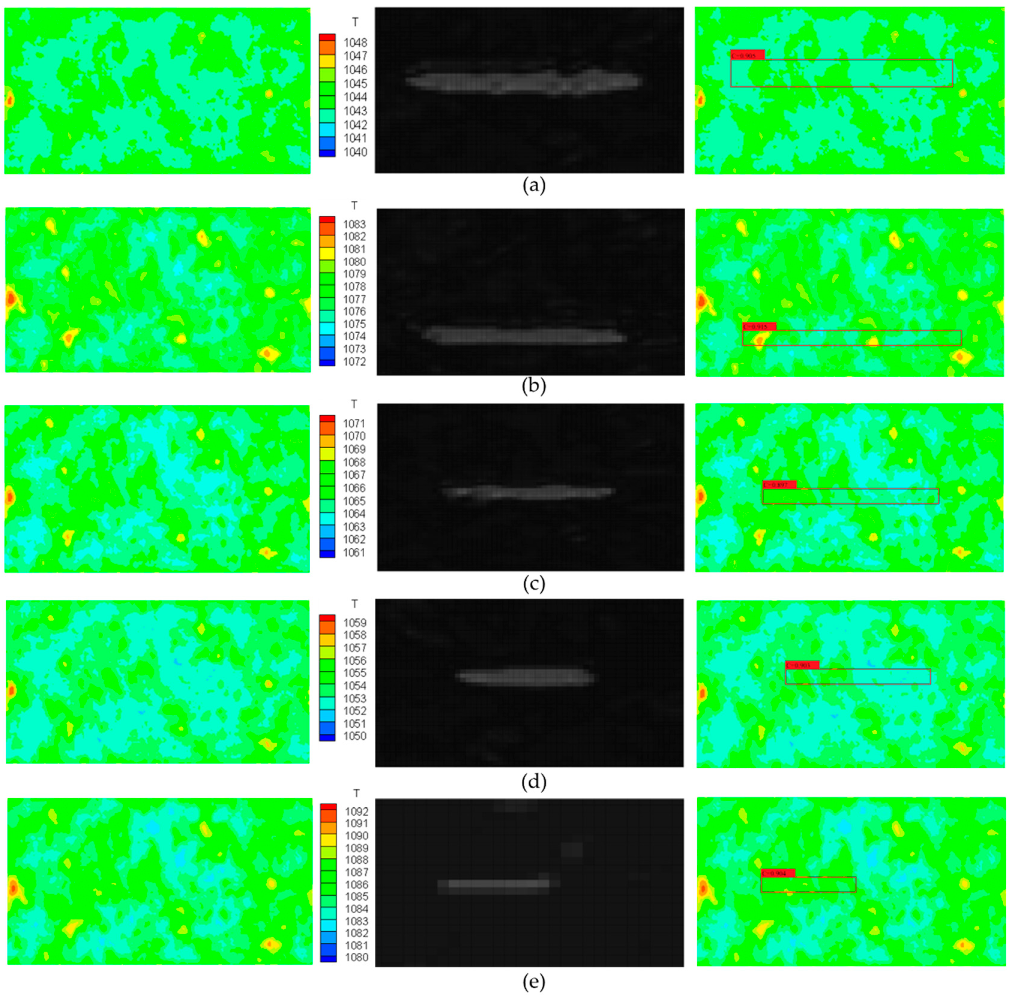
Figure 3 shows the detection results for different coating porosity and length of large scale cracks. The upper row is the temperature distribution of the coating with internal cracks. The temperature distribution here is intercepted by the numerical model in the state of heat exchange convergence, that is, it can be regarded as the final image surface temperature distribution. The temperature legend attaching the input image is generated based on the maximum and minimum temperature of the color temperature map, which will make the quality of the image reach the best possible level. The middle row is the feature visualization result, which maps the features in the convolution process to the pixel space to realize visualization, so as to observe the abstract process more intuitively. Since the model network is deep, an obvious convolution characteristic diagram is given. The correlation between the convoluted object and the convolution kernel can be calculated by the convolution kernel. The stronger correlation between the corresponding parts and the convolution kernel, the greater the convolution result will be. It can be seen from the figure that the deeper convolution layer makes the crack contour information fuzzy, but it can still show the area where the crack appears well. The bottom row is the detection results. The results show that cracks have been correctly detected with bounding boxes by using the detection scheme.

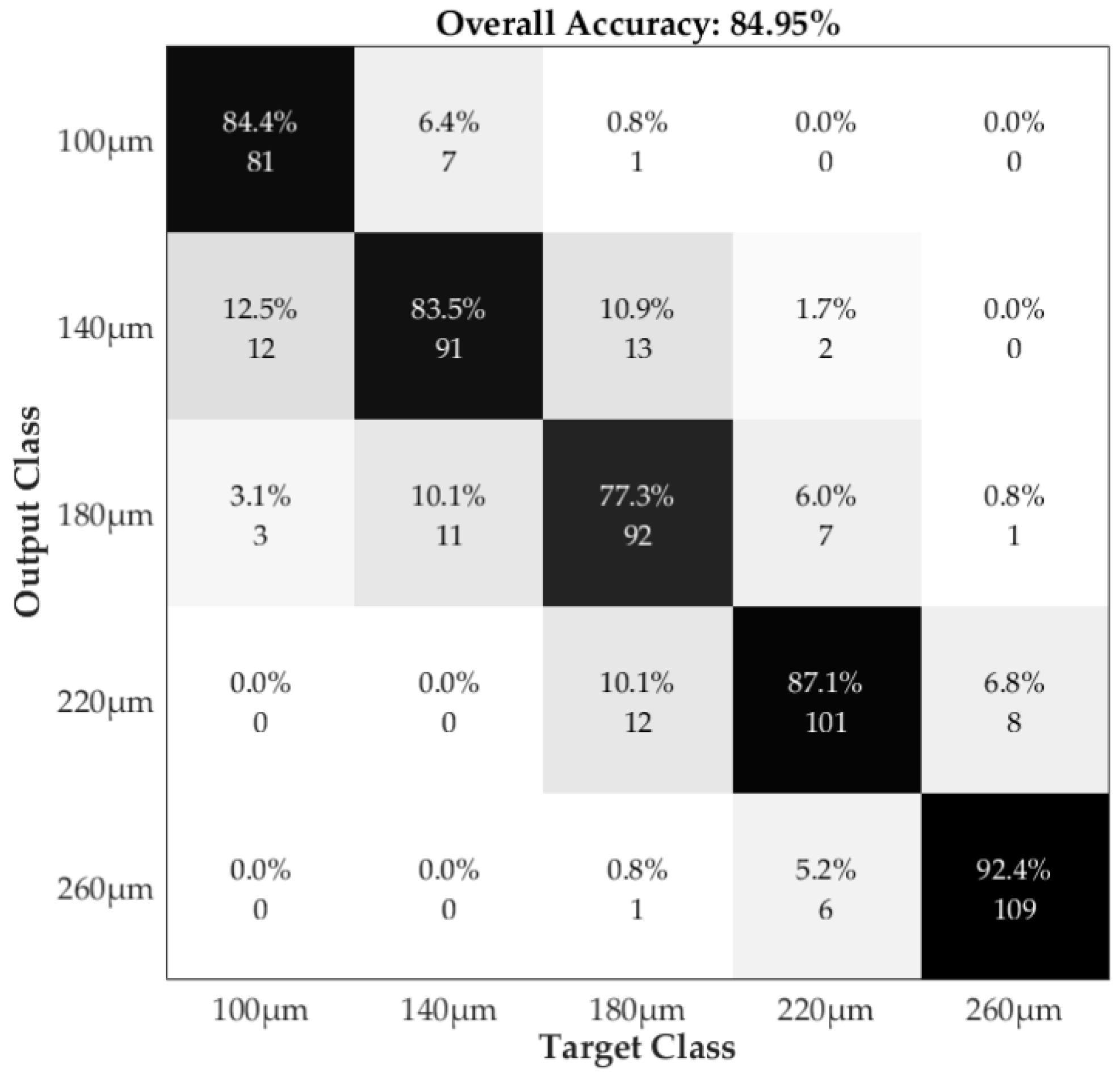
Figure 4 presents the confusion matrix of large-scale crack detection using the proposed algorithm. The confusion matrix is an analysis tool to measure the classification and prediction ability of the model. The rows of the confusion matrix represent the real value of each class and the columns represent the actual number of the predicted value of each class. The form of the confusion matrix is:

$$C=C\left[c_{ij}\right],i,j=1,2,\dots ,K$$

(14)

In Equation (14), C is the confusion matrix, K is the total classification number, c_ij represents the number of prediction results of classifying the class i samples represented by row i into the class j samples represented by column j. Therefore, the main diagonal elements (i = j) in the confusion matrix indicate that the classification is correct, and other non-main diagonal elements are miss-predictions. From the figure it can be seen that the overall accuracy of the proposed method is 84.95%. With the increase of crack length, the detection accuracy increases; especially when the crack length is more than 260 μm, the accuracy is more than 92%. This is because the longer crack has a greater influence on the whole region, which is more easily captured by the RPN network of MSE-Faster R-CNN in the training stage and regressed in the L₁ smooth stage.

4.4. Small Scale Crack Detection Experiments and Discussions

During the real monitoring, it is also necessary to observe the coating status of the local area at a high resolution. At this time, the shooting range will be narrowed. This requires the detection scheme to realize the diagnosis of small cracks with high accuracy. This section will describe such experiments.

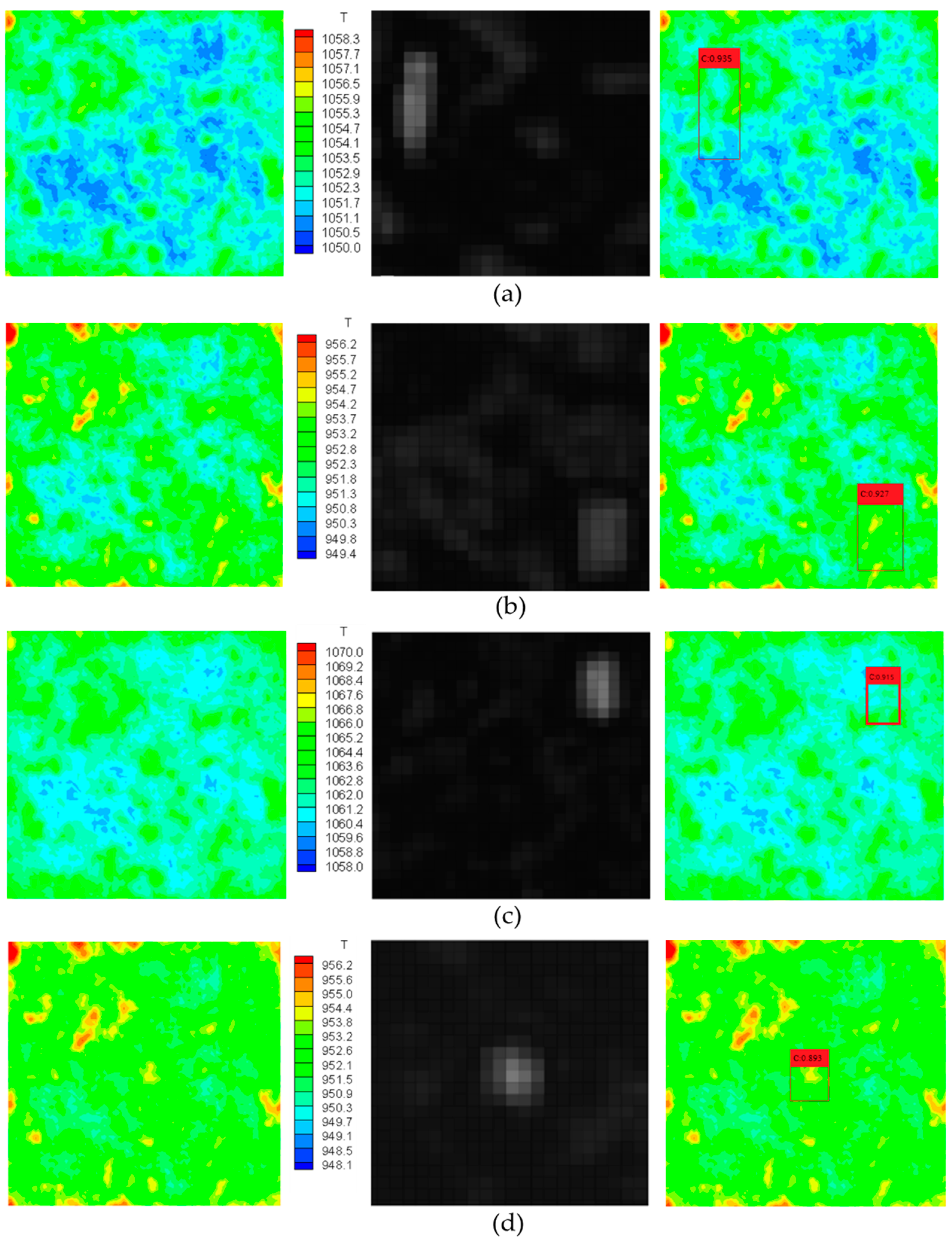
Figure 5 shows the surface temperature maps and the detection results of TBCs obtained under different coating porosity, length and position of small scale cracks. The crack length changes from 10 μm to 40 μm. The positions of cracks are at the center, upper left, upper right and bottom right of the image. The middle row is the feature visualization map. It can be seen that compared with Figure 4, the feature visualization effect of this figure is weakened, which shows that the detection accuracy of the algorithm is reduced in the case of small cracks, but it can still accurately identify the cracks. Through the proposed scheme, all the cracks are detected and located accurately with the anchor boxes. This is because MSE-Faster R-CNN has good global feature decoupling. After the convolution kernel fusion of different scales is introduced, some low activation neurons are successfully removed, and thus the feature extraction ability of the model is improved. Despite the similarities between small internal cracks and pores, there are still some differences. Pores are typically isotropic and have more uniform effects on the global, while cracks are anisotropic and have greater effects on the local. If MSE-Faster R-CNN can distinguish the differences between the two kinds of “holes” then this problem can be effectively solved.

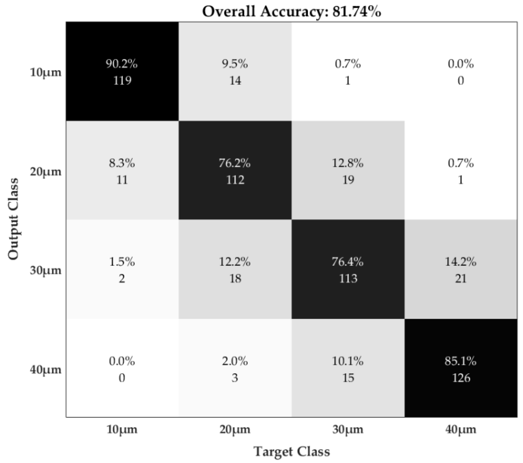
Figure 6 demonstrates the confusion matrix of the small scale crack detection. In general, the accuracy of crack detection is decreased compared with that of large cracks, from 84.4% to 81.74%. The detection accuracies are relatively high when there is no crack or the crack length is 40 μm, which are all around 85%. When the crack is 20 μm and 30 μm, some crack samples are easily confused with the nearby classes. Their accuracies are both less than 80%. The reason is as aforementioned in Figure 6: Small internal cracks are easily confused with pores due to their similarities in morphology. The change of temperature caused by a 10 μm crack is relatively weak. A similar conclusion can be drawn from another phenomenon; that is, compared with the results in Figure 5, the probability of confusion happening in a neighbor crack class is increased, but it is more difficult to confuse with further crack categories.

4.5. Comparative Analysis with Different Crack Detection Algorithms

To comprehensively evaluate the crack detection performance of MSE-Faster R-CNN, four other detection methods are used for comparison. In this part, VGG-19 network is set as the benchmark network, while Faster R-CNN, YOLOv4, Single Shot MultiBox Detector (SSD) [39], MMTL-NET [40], SegNet [41], and MSE-Faster R-CNN methods are used as target detection models for experiments. The location accuracy of different kinds of cracks is listed in

Table 3. Algorithms comparison in crack location accuracy.

Class\Method	Proposed	Faster R-CNN	YOLOv4	SSD	MMTLNet	SegNet
Non-crack	0.915	0.822	0.825	0.819	0.754	0.726
Large-scale cracks	0.923	0.850	0.861	0.830	0.780	0.731
Small-scale cracks	0.848	0.763	0.767	0.714	0.552	0.509
Average	0.898	0.819	0.823	0.782	0.698	0.650

. Among the methods, the proposed scheme has the best result (0.898). This shows that MSE-Faster R-CNN outperforms the original Faster R-CNN, and can better ensure the safety and economy of gas turbine operation. YOLOv4 is another state-of-art deep network, and it outperforms YOLOv3 with respect to detection accuracy as well as speed. It has a better result than Faster R-CNN (0.819). Unlike Faster R-CNN, YOLOv4 is a one-stage detector which also uses max-pooling and a mish activation to improve the accuracy. However, the feature extraction network of YOLOv4 is so deep that the information will be lost during training. The multi-scale model proposed in this paper fuses the convolution kernels of different visual fields, which enriches the diversity of features. Thus, the accuracy of the proposed method is higher than YOLOv4. The accuracy of the SSD algorithm is not as good as the previous deep learning algorithms (0.783). This might be because SSD are not sensitive enough to detect internal cracks. MMTLNET is a transfer learning network with adversarial training for 3D whole heart segmentation and it can extract multi-modality features and obtain the final segmentation results by fusing MRI and CT images. However, when the intersections of two or more foreground objects are not obvious like the pores and tiny cracks, its accuracy will be greatly reduced. Like the results shown in the last column, the accuracy of detection of small scale cracks decreases 0.2. Similar results also appear on SegNet, which is a state-of-art surface crack segmentation method, as discussed in the introduction. It can also be seen that when the crack length increases, the accuracy of each algorithm increases. This may be because the crack length and opening and closing degree in the large-scale crack dataset are more obvious than those of small-scale cracks.

Table 4. Algorithms comparison in crack detection accuracy.

Class\Method	Proposed	Faster R-CNN	YOLOv4	SSD	MMTLNet	SegNet
Non-crack	0.821	0.747	0.764	0.783	0.665	0.626
Large-scale cracks	0.864	0.814	0.802	0.726	0.699	0.638
Small-scale cracks	0.712	0.650	0.668	0.677	0.640	0.606
Average	0.806	0.739	0.747	0.732	0.673	0.627

shows the comparison of crack detection accuracy of various algorithms. The conclusion is close to Table 3: the algorithm proposed in this paper still achieves the best performance (0.806). It can be seen that the detection accuracy of each algorithm has decreased compared with the positioning accuracy, which is also consistent with the conclusions in Table 2. In addition, the detection results of large-scale crack data set are better than small-scale cracks, which is still in line with the previous conclusions.

4.6. Experiments and Analysis of Coating Lifetime Estimation

As a durable part of the turbine blade, its economy should be considered in the real service process. The service lives of turbine blades can be greatly prolonged by removing coating and re-spraying. Therefore, it is also of significance to accurately estimate the TBCs lifetime to determine the operation decisions for gas turbines without causing irreparable damage to the hot components.

In order to quantitatively evaluate the deviation between the predicted results and the ground truth, the Root Mean Square Error (RMSE) is adopted: which is defined as:

$$RMSE=\sqrt{\frac{1}{n}{\displaystyle \sum }_i^n{\left(R_i-P_i\right)}^2}$$

(15)

In Equation (15), n is the total number of predictions, R_i is the real RUL of the i_th sample. It is given by the finite element simulation results on the numericial model. P_i is the predicted RUL of the i_th sample using the lifetime prediction methods.

The physical model, RVM model and information entropy fusion model are compared by predicting the RUL of the TBC.

Table 5. Comparison of RMSEs of different lifetime prediction methods.

Methods	RMSE	Time Cost
Single-Physical model	8.7	0.95 s
Single-RVM	3.3	1.26 s
Information Entropy	2.7	1.63 s

lists the comparison of RUL prediction results using single method and weighted fusion algorithms. It can be seen that the fusion method based on information entropy has the best effect, which is superior to the other two methods in terms of the RMSE. The time cost of using the single detection method is shorter than that of the fusion method. However, all the time consumption periods for these methods are less than 2 s, which is acceptable for on-line monitoring of coatings with a low sampling rate.

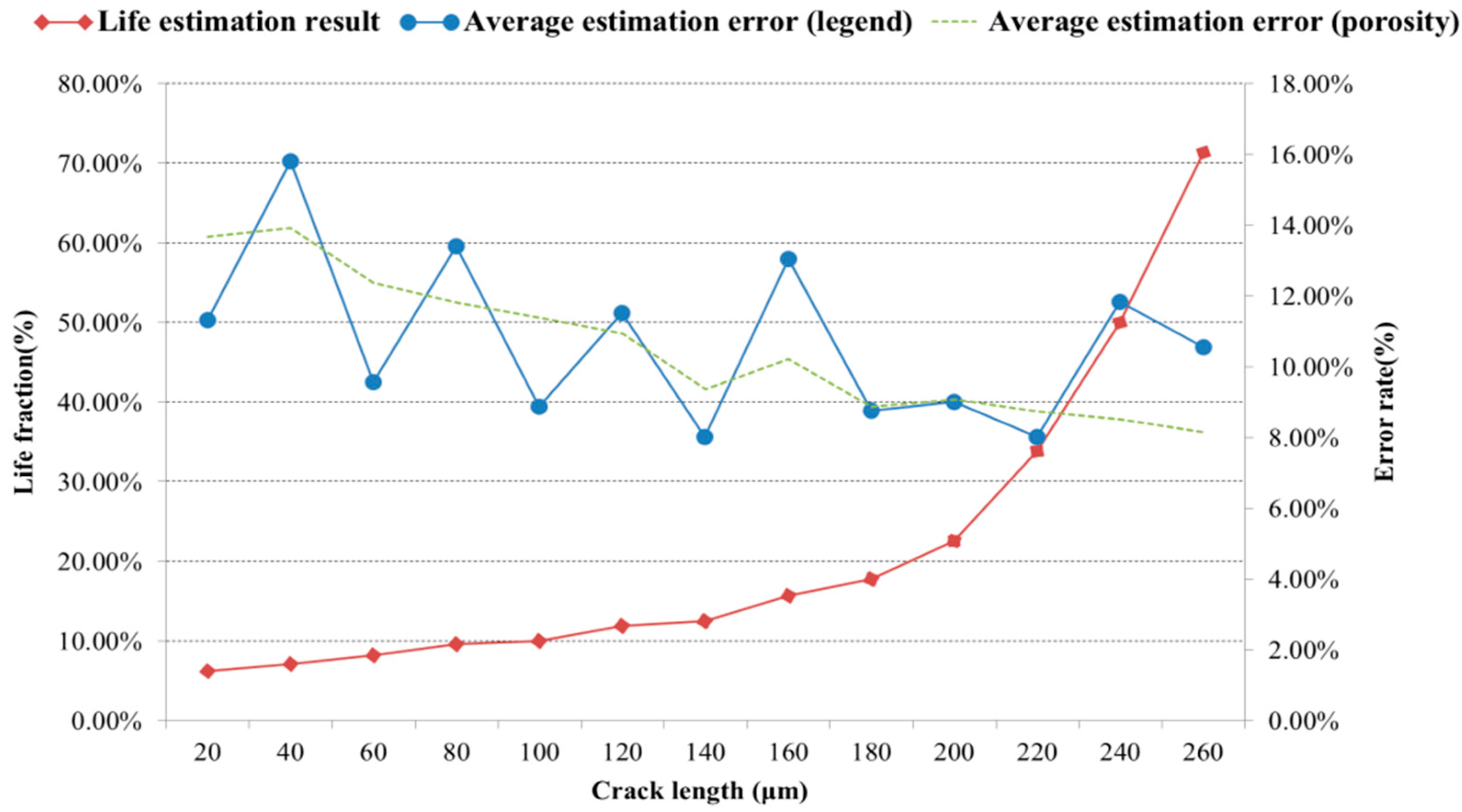
The lifetime estimation result calculated by the fusion model is depicted in Figure 7. The result reveals that the effect of crack length on coating lifetime is nonlinear. When the crack length is between 20 μm and 200 μm, the coating lifetime fraction does not increase significantly, but when the crack length is above 220 μm, the coating lifetime has entered a sharp downturn, which reflects that the crack length has an exponential effect on the internal stress. This conclusion is basically consistent with the detection accuracy given by Figure 5 since when the crack length is more than 220 μm, the detection accuracy also sees a great improvement. The error rate of different porosities and temperature legends in variation of crack lengths is also described in the figure. The temperature legend represents the range of the whole picture. When the temperature legend is set larger and the shooting range remains (as is the case in this study), its resolution will be lower, providing disturbance for lifetime prediction. The temperature legend in this lifetime prediction experiment is set between 1020 °C and 1080 °C initially, and expanded to between 940 °C and 1080 °C. The porosity is set at 25% initially, and decreased to 5% by the end. From the figure it can be seen that all detection conditions of the error rates are below 15%. The distribution of error rates is nearly random but generally the error rate of changing porosity is lower than that of changing temperature legend. That is probably because a larger legend will decrease the quality of an infrared image. An appropriate setting legend will make the contrast of the image placed in the best position, which will make it easier for the trained MSE-Faster R-CNN detector to capture the features reflecting the cracks, so that the detection accuracy will be higher.

5. Conclusions

To solve the problem that the existing crack detection methods have poor generalization ability and low accuracy for internal cracks, a detection scheme based on MSE-Faster R-CNN was proposed. Firstly, VGG-19 was employed as the baseline network to select crack candidate regions. Secondly, a novel design of MSE-Faster R-CNN detector was utilized to conduct feature fusion, classify the state of the candidate region and measure the crack position and length. The performance of the method was validated by different scales of numerical dataset. The following conclusions can be drawn:

• By comparing different state-of-art methods, experimental results showed that the internal crack detection by the proposed scheme had best performance at both large and small scale. The accuracy can reach 0.898 in location detection and 0.806 in crack detection. The proposed scheme can distinguish the differences between the small internal cracks and pores, but the detection error rate also increases.
• Based on the localized diagnosis of cracks and the fusion lifetime estimation algorithm, the coating lifetime can be preliminarily evaluated by the crack detection results. The fusion lifetime estimation result with different crack lengths had acceptable RMSE (2.7) as well as time cost (1.63 s).
• In future, further research should be promoted to detect other characteristics of internal cracks, such as density, morphology, crack orientation, etc. Current research mainly focuses on the diagnosis of a single crack. In reality, there may be multiple cracks at the same time. Due to the heat flow coupling effect between the cracks, this effect will have a complex impact on the temperature distribution. Current research regards the crack shape as an ellipse and regards crack orientation as almost straight, but in reality, there are other crack growth patterns and orientations. Such different growth patterns and orientations will have significant effects on the temperature distribution. In addition, the proposed scheme should be tested and improved using real data to validate the feasibility. Although transferring learning is used, which is helpful to the results, the existing datasets still need to be expanded at different scales.