Visual Scratch Defect Detection System of Aluminum Flat Tube Based on Cubic Bezier Curve Fitting Using Linear Scan Camera

Abstract

This paper presents a scratch detection system based on a cubic Bezier curve fitting using a linear scan camera. The objective was to detect the scratch defects of an aluminum flat tube stably in real-time under complex uncertain background noise. To that end, according to the features of the input image of the linear scan camera and the scratch defects, the proposed method first segmented the input image to ten equal sections in a longitudinal direction, and for every section, OTSU thresholding and morphological filtering were used to reduce the background noise. After the image preprocessing, every section image was projected along a vertical direction to form a vertical histogram. After that, for each point of every vertical histogram, a novel curve fitting method based on the Monte Carlo method was employed to calculate the best fitted Bezier curve. All the curvatures of the middle point of the best fitted Bezier curves then formed a curvature curve, and the scratches were located by finding the peaks of the curvature curve. Next, the result of the ten sections were fused to find the final positions of the scratches. The experimental results based on the linear scan camera that captured the image of flat tubes on a moving speed of 2m/s showed that the proposed method can detect the scratch defects under complex background noise with a high success rate in real-time.

1. Introduction

A microchannel aluminum flat tube is a thin-walled porous flat tubular part formed by hot extrusion of a refined aluminum rod and a surface zinc spraying anti-corrosion treatment. It is the core component of a parallel flow heat exchanger (as shown in Figure 1), which has attracted the interest of many scholars in the field of thermal engineering lately [1,2,3]. Because of its small volume, high efficiency, compactness, light weight and many other advantages, it is favored by the automobile heat exchanger industry, and has been widely used in automobile air conditioning systems, while its application has been gradually expanding to the field of household air conditioning.

Due to the high technical content and difficult production of the microchannel aluminum flat tube, it is easy to form a variety of surface defects in the production process. These surface defects including pits, holes, scratches et al. (as shown in Figure 2). Since any minor surface defect may lead to a refrigerant leakage during actual use, resulting in the scrapping of the whole heat exchanger, manufacturers are eager to find solutions for the surface defects detection. Some of the defects such as pits and holes can be detected successfully by using machine vision, but the detection of scratches remains an unsolved problem. In this paper, a new scratch defects detection algorithm in the complex clutter background was proposed to tackle this problem.

There are three reasons making it difficult to detect the scratches of a microchannel aluminum flat tube. First, there are great differences in the depth of scratches, where some scratches are deep while some are shallow, causing large differences between different scratches. Secondly, there are many background clutters in the image. For example, oil stains will remain on the surface during the production process, which makes the imaging situation of the flat tube surface complex and changeable. Finally, the length of the flat tube is different: the length of the scratches may be as long as the whole length of the tube, with the longest being up to 800 mm, while the shortest is only 200 mm. As a result, when using deep learning algorithms, such as CNN or RNN, which rely on unified database training, they do not perform as well as in other application cases.

To detect surface defects in industrial production, different kinds of advanced technologies have been developed by scholars and engineers. Wang et al. [4] proposed a Bayesian dynamic linear model to achieve real-time high speed rail defects detection. Horan et al. [5] and Arjun et al. [6] employed a pulsed eddy current to find surface defects in metal material surfaces and complex structures. Peng [7] and Huang [8] employed eddy current pulsed thermography to detect defects of metal material. Sunny et al. [9] employed a low-frequency radio frequency identification (RFID) system to characterize marine atmospheric corrosion of steel materials, and Zhang summarized and highlighted the difficulties and best performance methods of passive RFID antenna systems and sensors. Tehranchi et al. [10] used magnetic flux leak technique to detect crack like defects. Baek et al. [11] proposed a line-scan technique for hyperspectral imaging combing a four mirror system to observe a round spinning object to detect surface defects.

Although the techniques mentioned above have some successful applications, the most widely used methods of defect detection are based on machine vision, and the key part of these machine vision system is the detection and recognition algorithm. In order to achieve robust defects detection, many useful algorithms have been proposed by scholars all over the world. Zhang, et al. [12] used the wavelet smoothing method to reduce background noise from input images, and then the Otsu threshold method was used for segmentation, and finally a Support Vector Machine was used for classification. In the study by Song et al. [13], a local binary pattern method for adjacency evaluation was proposed, which modified the threshold scheme of the completed local binary pattern by constructing the adjacency evaluation window. Liu et al. [14] proposed a non-subsampled shearlet transform and the kernel locality preserving projection (NSST-KLPP) to identify surface defects of aluminum strips. In this work, 230 scratch defect samples were used and the recognition rate is 95.65%. Li et al. [15] used a deep learning based YOLO (You Only Look Once) network to detect the different surface defects on steel strips, and achieved a 99% successful detection rate with high speed (83FPS). He et al. [16] used a baseline convolution neural network to generate feature mapping, proposed a multi-level feature fusion network to locate defect details, and then used a regional suggestion network (RPN) to generate regions of interest. Huang et al. [17] developed an automatic system to detect surface scratches on tubes of high curvature. The algorithm was divided into two steps, respectively, designing a two-dimensional directional filter to enhance the contrast between the scratches and background, and using an improved adaptive threshold method to automatically detect the edges of scratches on the filtered image. He et al. [18] proposed a semi-supervised learning method combing the convolutional autoencoder and semi-supervised generative adversarial network to detect and classify the defects on the hot rolled plates. Zhang et al. [19] utilized attention mechanism and unified detection to address the challenging defects on an aluminum profile surface.

Although different kinds of machine vision methods have been proposed to detect defects on material surface as mentioned above, none of them are suited to detect the scratch defects of the aluminum flat tube due to the reasons explained above. In order to address this problem, a new scratch detection and location system based on a cubic Bezier curve fitting using a linear scan camera was proposed in this paper.

The novelties of the paper are:

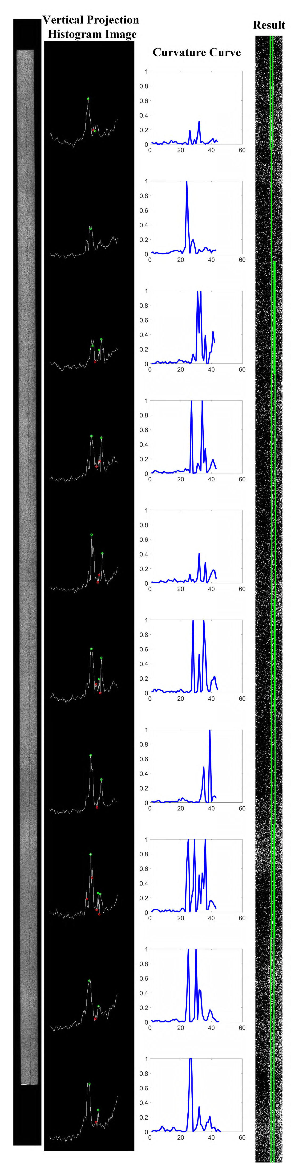
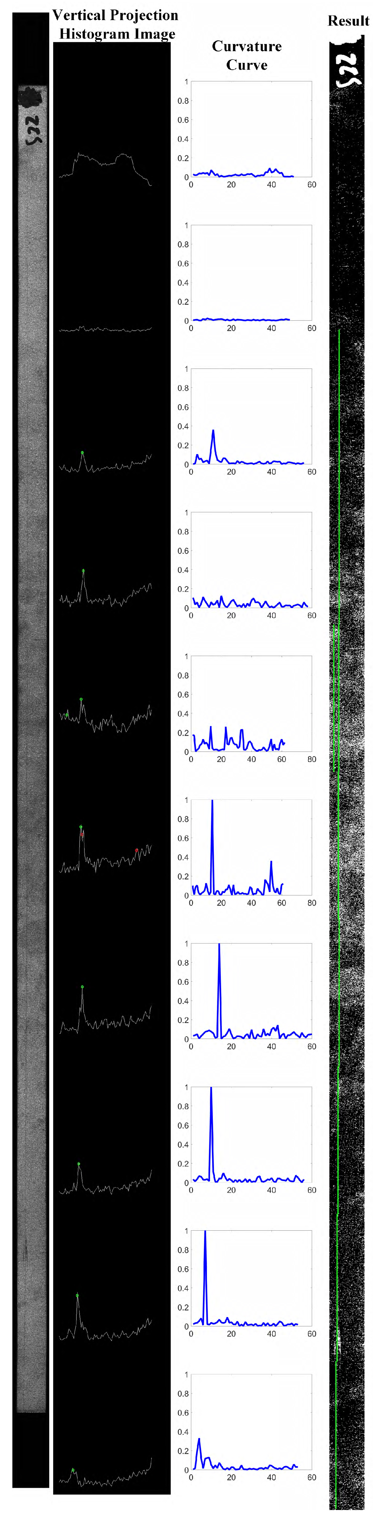
• A new scratch detection and location system was proposed to find local maximums based on Bezier curvature calculation and curve fitting. By using this technique, the stability and accuracy of curvature peak localization in the complex clutter background was improved significantly.
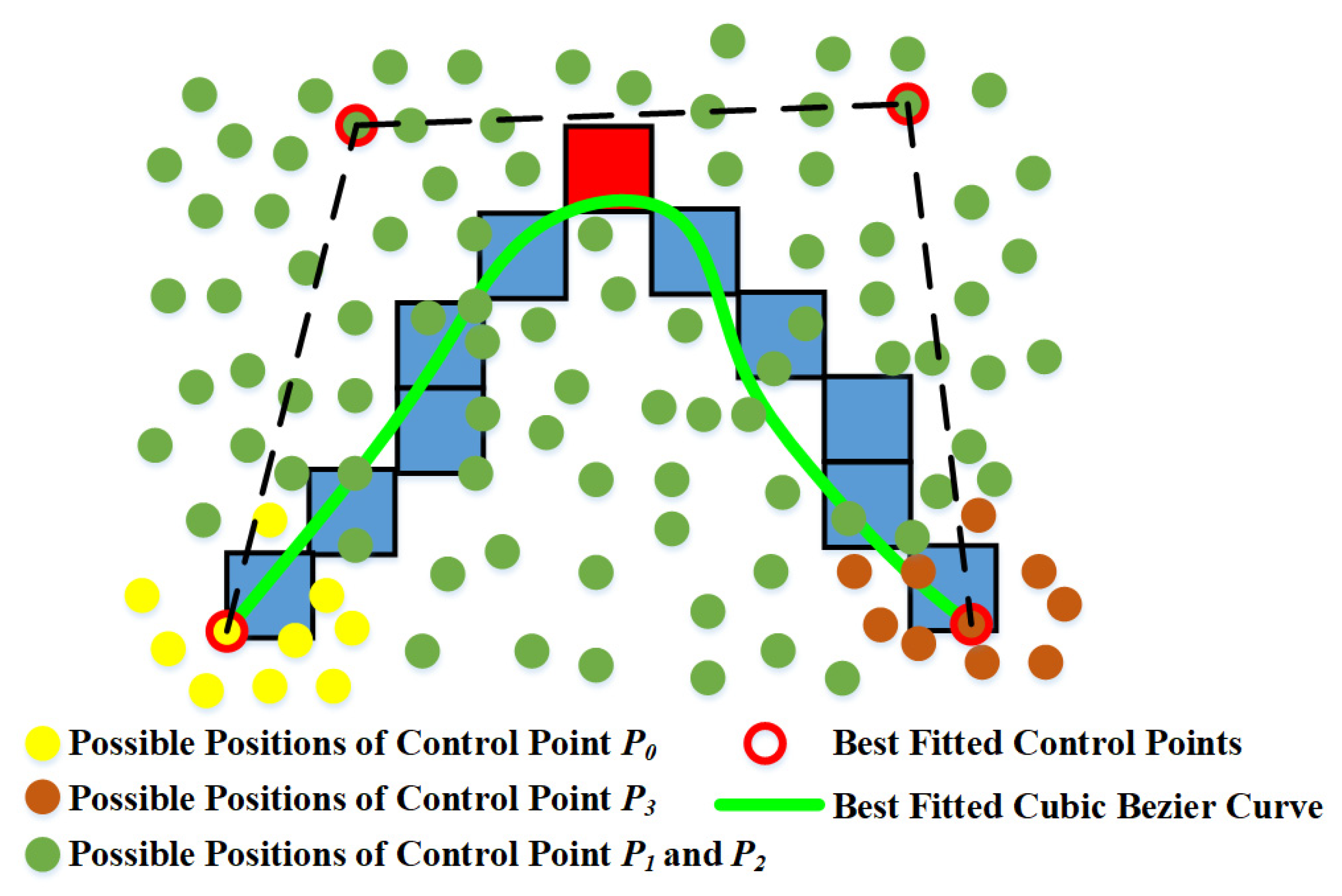
• Monte Carlo sampling was used to find the optimal four control points location of the Bezier curves. By using the Monte Carlo scheme, the optimal control points can be found in a less time-consuming way, which is important in real-time application.
• The scratch detection using the proposed method, achieved in real-time processing, based on a linear scan camera.

The paper is structured as follows. The next section explains the details of the proposed scratch detection method including image preprocessing, Bezier curve presentation, Monte Carlo sampling and Bezier curve curvature and local maximums extraction. Section 3 introduces the parameters setting, experimental results and analysis. Section 4 outlines the conclusions and future research.

2. The Proposed Method

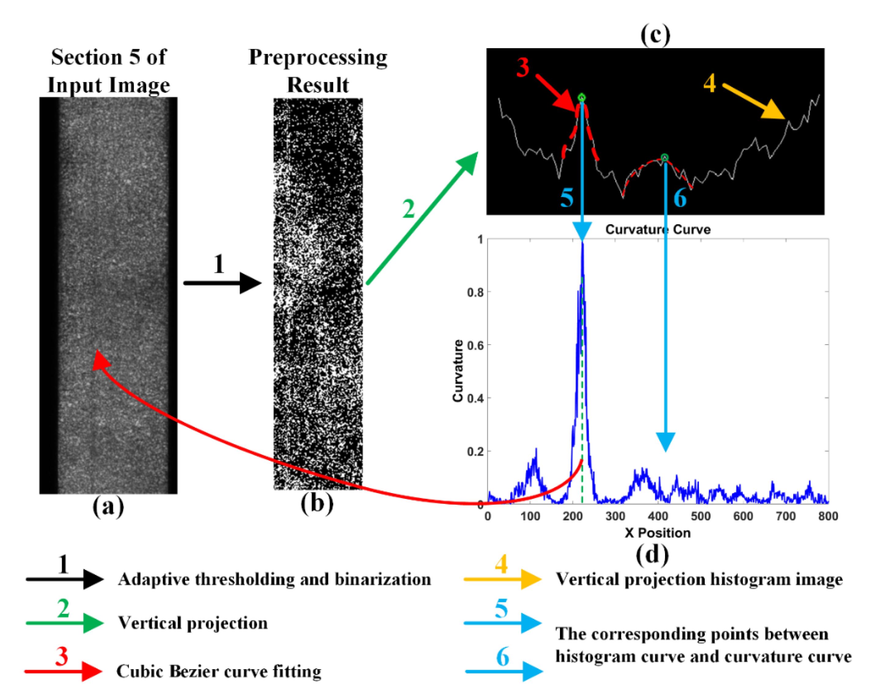
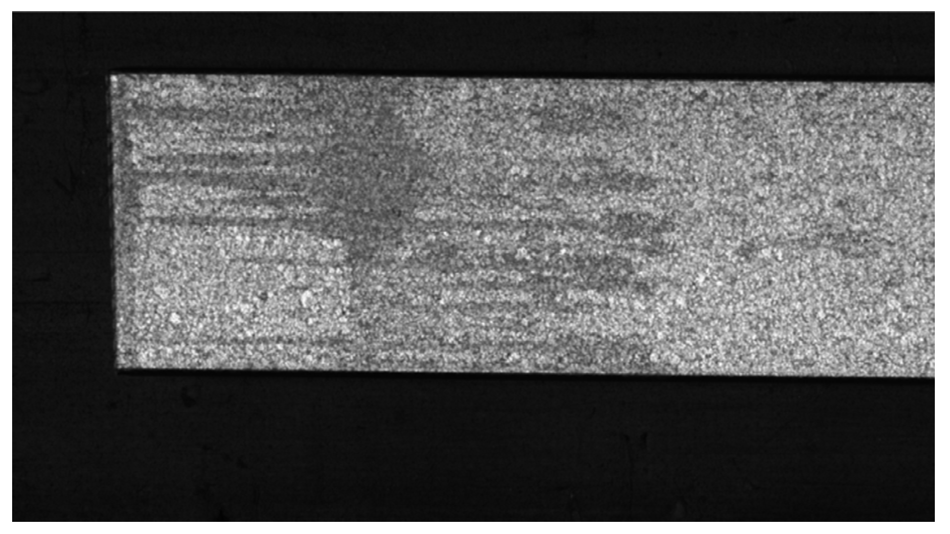
2.1. Overview of the Proposed Method and Image Preprocessing

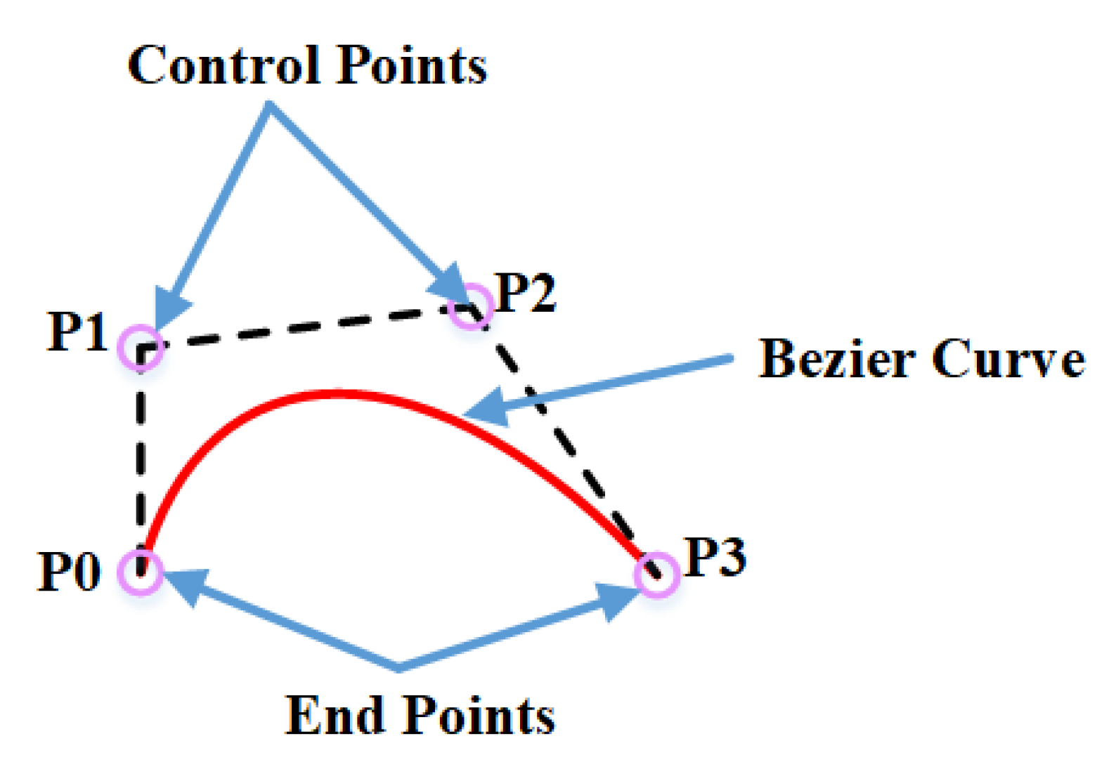
According to the characteristics of production technology, flat tubes are often narrow and long. For example, the whole image size of Figure 3 is 600 × 23,000, and the scratches are often longitudinal, and there will be a small deflection angle at the same time. In order to detect the scratches effectively, appropriate image preprocessing methods are needed. In this work, the input images are segmented into ten equal length sections (as seen in Figure 3), and in every section, the scratch detection algorithm is applied, and then all the ten results are fused together to yield the final result.

For every section of the input image, OTSU thresholding [20] was used at the first step, and then morphological filtering was applied to reduce the background clutters, as seen (b) in Figure 4. After that, a novel method combing the cubic Bezier curve fitting and Monte Carlo random sample was employed for scratch detection. The image after preprocessing then used to construct a vertical projection histogram, as seen (c) in Figure 4. Since it is still hard to locate the defect position in the histogram curve due to background noise, the curvature of every point in the histogram curve was calculated by the Bezier curve fitting and the construction of a curvature curve, as seen in (d) in Figure 4, which is much easier for detecting the scratches. Figure 4 shows the overview of the proposed method in processing the fifth section of the input image.

2.2. Bezier Curve

Assume that the vertical projection histogram curve consists of a set of points $\left\{C{P}_m\right\} 1\le m\le M$, where $M$ is the number of total points in the curve. For every point in curve, a point group of $C{P}_m$ including $2L+1$ points can be expressed as follows:

$$\begin{array}{c} \left\{C{P}_{m+j}^s\right\} 1\le m\le M -L\le j\le L\end{array}$$

(1)

The point $C{P}_m$ is the center point of the sub points set $C{P}_{m+j}^s$, which means there are $L$ points before $C{P}_m$, and also $L$ points after $C{P}_m$ (see Figure 5). If we can construct a smooth curve that fit all the sub points well, and the curvatures in the fitted curve can be calculated precisely and easily, then all the curvatures of all sub points set can construct a new “curvature curve”, which can be used to estimate the local maximums (normally means the positions of scratches). In this situation, the key problem turns to find a curve fitting algorithm to the points group $C{P}_{m+j}^s$.

In order to address this problem, a curve fitting method based on Bezier curve and Monte Carlo sampling is proposed.

A Bezier curve, which is widely used in many applications, is a kind of parametric curve, in which a group of discrete “control points” defines a smooth, continuous curve by means of a formula.

A degree n Bezier curve can be formulated:

$$\begin{array}{c} P\left(t\right)={\displaystyle \sum _{i=0}^n}{P}_i{B}_{i,n}\left(t\right) t\in \left[0,1\right]\end{array}$$

(2)

where $P_i$ means the control points of the curve, $n$ means the degree, and $t$ is the parameter to control the smoothness of the curve. The basis function, $B_{i,n}\left(t\right)$, is the Bernstein polynomials of degree n defined explicitly by:

$$\begin{array}{c} B_{i,n}\left(t\right)=C_n^i{t}^i{(1-t)}^{n-i}=\frac{n!}{i!\left(n-i\right)!}{t}^i{(1-t)}^{n-i}\end{array}$$

(3)

In this study, the cubic Bezier (see Figure 6), that is $n=3$, was used after considering both the accuracy and efficiency. In a cubic Bezier curve, four points are required, including two points which are not on the curve (control points) while the other two are on the ends of the curve (end points).

The problem mentioned in the last section of finding the optimal curves of every sub point set $C{P}_{m+j}^s$, turned to finding four optimal control points that define the corresponding Bezier curve. This is a typical proximity point optimization problem, which some scholars have already studied in depth from a mathematical perspective [21,22]. Giving $2L+1$ points, an obvious way to find a group of four optimal control points is to perform an exhaustive search of the whole space, but this method was not a good choice. In this study, the Monte Carlo sampling method was used to optimize the location of the control points quickly.

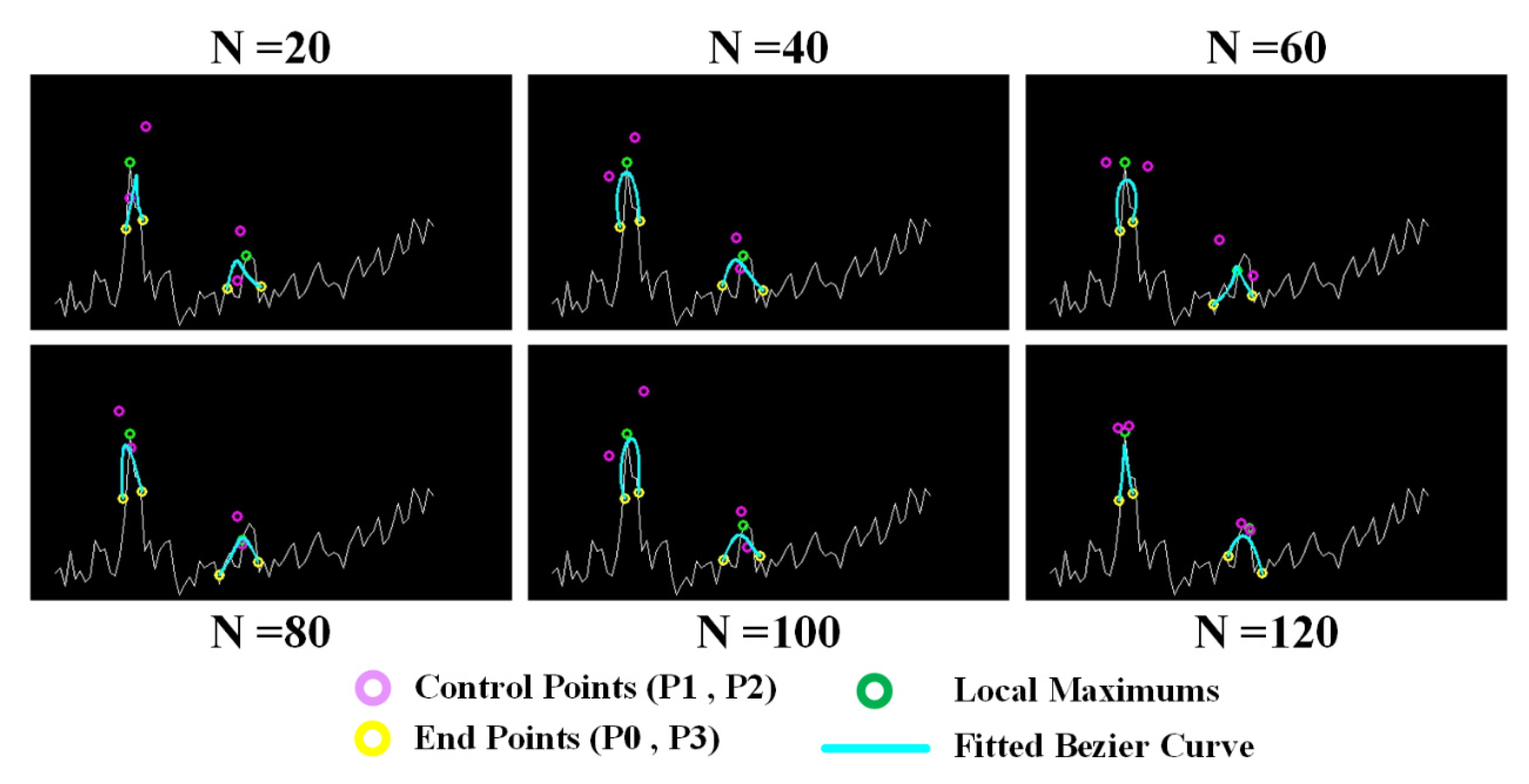
2.3. Monte Carlo Sampling

The Monte Carlo method is a computational algorithm, the underlying concept of which is using randomness to solve problems that might be deterministic in principle. It is often used in optimization, numerical integration, and other related application.

The fitting problem associated with using the cubic Bezier curve in this application can be formulated as:

$$\begin{array}{c} \underset{x\in X}{min}\left\{f\left(x\right)≔E\left[F\left(x,\xi \right)\right]\right\}\end{array}$$

(4)

where $F\left(x,\xi \right)$ is the objective function of two vectors $x\in R^n$ and $\xi \in R^d$. In this paper, $x$ is a given point set, and $\xi$ means a candidate sub curve $\left\{P{(\omega ,t)}_m^s\right\}$, the vector $\omega$ is a group of randomly generated control points which can define a cubic Bezier curve, and $x$ refers to a given sub points set $\left\{C{P}_{m+j}^s\right\}$. The function $F\left(x,\xi \right)$ is formulated as:

$$\begin{array}{c} F\left(x,\xi \right)={\displaystyle \sum _{j=0}^{2L+1}}|P{(\omega ,t)}_m^s-C{P}_{m+j}^s{|}^2\end{array}$$

(5)

The goal of this method is to calculate the optimal fitting Bezier curve of the given point group through Monte Carlo sampling by using the least square method.

For every $\left\{C{P}_{m+j}^s\right\}$, each candidate sub curve can be generated using the random control points vector ${\omega }^{\zeta },\zeta =1,2\dots N$ where $N$ is the total candidate number (or sample number, and the proof of minimum sample number can be found in next section). A candidate curve can be expressed as the following:

$$\begin{array}{c}{P}_{\zeta }{({\omega }^{\zeta },t)}_m^s={\displaystyle \sum _{i=0}^3}{P}_i{({\omega }^{\zeta })}_m{B}_{i,3}\left(t\right)=\left[\begin{array}{cccc}{t}^3& t^2& t& 1\end{array}\right] \left[\begin{array}{cccc}-1& 3& -3& 1\\ 3& -6& 3& 0\\ -3& 3& 0& 0\\ 1& 0& 0& 0\end{array}\right] \left[\begin{array}{c}{\omega }_{0m}^{\zeta }\\ {\omega }_{1m}^{\zeta }\\ {\omega }_{2m}^{\zeta }\\ {\omega }_{3m}^{\zeta }\end{array}\right]\end{array}$$

(6)

The four control points ${\omega }_{0m}^{\zeta }$, ${\omega }_{1m}^{\zeta }$, ${\omega }_{2m}^{\zeta }$ and ${\omega }_{3m}^{\zeta }$ are random variables, and they have different distribution areas:

$$\begin{array}{l}{\omega }_{0m}^{\zeta }\in \left[C{P}_{m-L}^s-T_0,C{P}_{m-L}^s+T_0\right]\\ {\omega }_{1m}^{\zeta }\in \left[T_{min}-T_0,T_{max}+T_0\right]\\ {\omega }_{2m}^{\zeta }\in \left[T_{min}-T_0,T_{max}+T_0\right]\\ {\omega }_{3m}^{\zeta }\in \left[C{P}_{m+L}^s-T_0,C{P}_{m+L}^s+T_0\right]\end{array}$$

(7)

where $T_0$ is a tolerance interval threshold of the certain range, and $T_{min}$, $T_{max}$ are described as:

$$\begin{array}{c}{T}_{min}=\min \left\{C{P}_{m+j}^s\right\}-L\le j\le L\\ T_{max}=\max \left\{C{P}_{m+j}^s\right\}-L\le j\le L\end{array}$$

(8)

Figure 7 explained Equation (7) in a more detailed way. $P_0$ is the start control point and $P_3$ is the end control point, and they are expected to appear within a relatively small region centered in the related point of the given points ($C{P}_{m-L}^s$ and $C{P}_{m+L}^s$), while $P_1$ and $P_2$ will have the chance to be in any position of the whole region defined by $\left\{C{P}_{m+j}^s\right\}$.

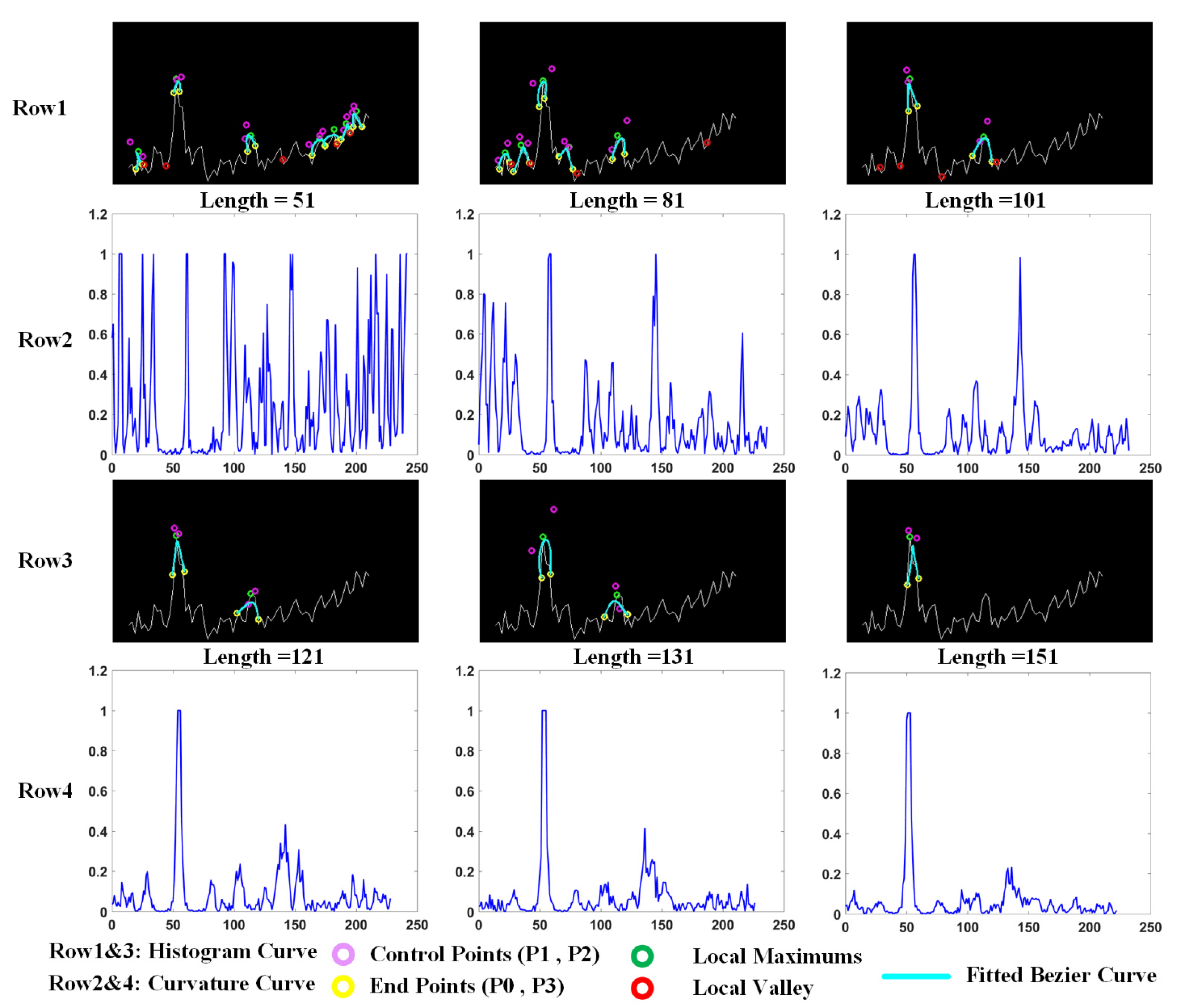
2.4. Minimum Sampling Number

Suppose $n$ times of the independent random sampling are carried out, in which the probability of correctly selecting the best fitting Bezier curve for each success is $p$, and the probability of failure is $1-p$; if X represents the success in $n$ independent random sampling times, then $X$ is a binomial random variable with parameters $\left(n,p\right)$, and its probability density function is:

$$\begin{array}{c} p\left(i\right)=C_n^i{p}^i{(1-p)}^{n-i}\end{array}$$

(9)

Then the mathematical expectation of the binomial random variable $X$ is:

$$\begin{array}{ll} E\left[X\right]& ={\displaystyle \sum _{i=0}^n}ip\left(i\right)={\displaystyle \sum _{i=0}^n}i{C}_n^i{p}^i{(1-p)}^{n-i}\\ & ={\displaystyle \sum _{i=0}^n}\frac{in!}{\left(n-i\right)!i!}{p}^i{(1-p)}^{n-i}\\ & ={\displaystyle \sum _{i=0}^n}\frac{n!}{\left(n-i\right)!\left(i-1\right)!}{p}^i{(1-p)}^{n-i}\\ & =np{\displaystyle \sum _{i=0}^n}\frac{\left(n-1\right)!}{\left(n-i\right)!\left(i-1\right)!}{p}^{i-1}{(1-p)}^{n-i}\\ & =np{\displaystyle \sum _{i=0}^n}{C}_{n-1}^k{p}^k{(1-p)}^{n-1-k}\\ & =np{[p+\left(1-p\right)]}^{n-1}\\ & =np\end{array}$$

(10)

That is, the average number of successes of $n$ times of independent random sampling is $n$ multiplied by the probability of each success, so if $n$ times of independent random sampling are done, at least one success can be expressed as:

$$\begin{array}{c} E\left[X\right]\ge 1\iff np\ge 1\iff n\ge \frac{1}{p}\end{array}$$

(11)

If a control point falls within a 5 × 5 neighborhood centered on the correct control point position, it is approximately correct, and the sampling points are uniformly distributed in the sampling space. The minimum required sampling times are then:

$$\begin{array}{c} n\ge \frac{1}{p}=\frac{N_w\times N_h}{5\times 5}\end{array}$$

(12)

where $N_w$ is the width of the sampling region and $N_h$ is the height of the sampling region.

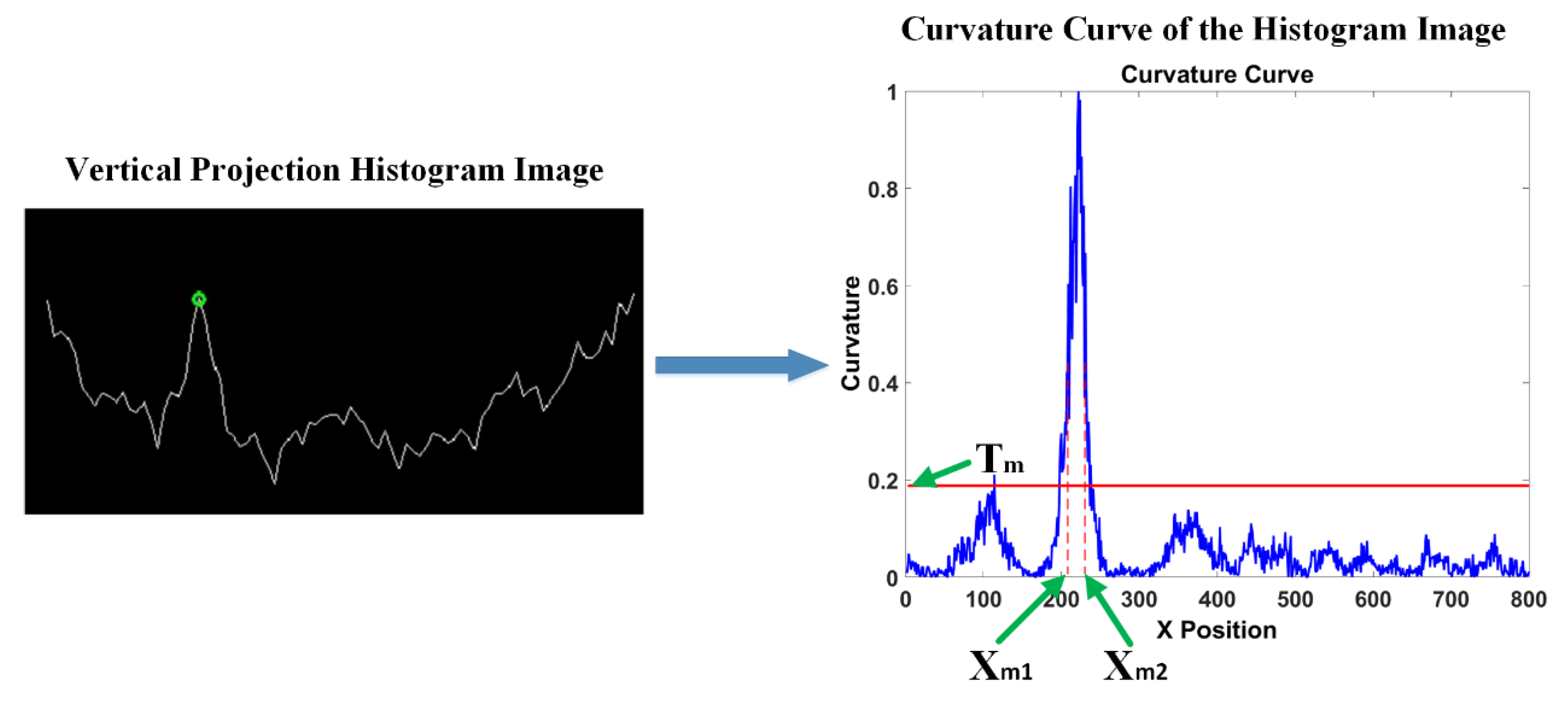
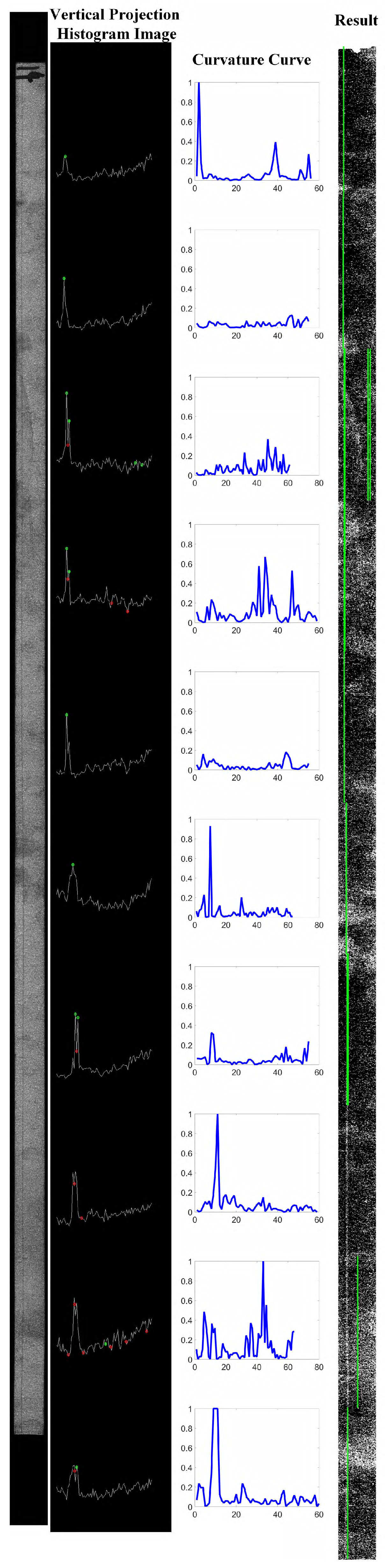
2.5. Bezier Curvature Calculation and Peak Location

By employing the method of the previous section, a group of control points that fit the given sub points set $\left\{C{P}_{m+j}^s\right\}$ best can be found, represented as $\left\{P_i^{best},i=0,1,2,3\right\}$. Having the optimal control points, the curvature at any point in the corresponding Bezier curve can be calculated as following:

$$\begin{array}{c} K\left(t\right)=\frac{\left|P^{\prime }\left(t\right)\times P^{″}\left(t\right)\right|}{|P^{\prime }\left(t\right){|}^3}\end{array}$$

(13)

where $P^{\prime }\left(t\right)$ represents the first derivative and $P^{″}\left(t\right)$ represents the second derivative of the Bezier curve. They can be calculated by the following equations:

$$\begin{array}{c} P^{\prime }\left(t\right)={\displaystyle \sum _{i=0}^n}{P}_i^{best}{B_{i,n}}^{\prime }\left(t\right) =n{\displaystyle \sum _{i=1}^n}(P_i^{best}-P_{i-1}^{best})B_{i-1,n-1}\left(t\right)\end{array}$$

(14)

$$\begin{array}{c}{P}^{″}\left(t\right) =n\left(n-1\right){\displaystyle \sum _{i=0}^{n-2}}(P_{i+2}^{best}-2P_{i+1}^{best}+P_i^{best})B_{i,n-2}\left(t\right)\end{array}$$

(15)

They can be written more detailed as:

$$\begin{array}{c}{P}^{\prime }\left(t\right)=3[\left(P_1^{best}-P_0^{best}\right)\left(1-t{)}^2+\left(P_2^{best}-P_1^{best}\right)t\left(1-t\right)+\left(P_3^{best}-P_2^{best}\right)t^2\right]\end{array}$$

(16)

$$\begin{array}{c}{P}^{″}\left(t\right) =6\left[\left(-P_0^{best}+3P_1^{best}-3P_2^{best}+P_3^{best}\right)t+\left(P_0^{best}-2P_1^{best}+P_2^{best}\right)\right]\end{array}$$

(17)

Each points set has $2L+1$ points; the middle point is $C{P}_m$ and $L$ points before $C{P}_m$ as well as $L$ points after $C{P}_m$, which means the curvature at $K\left(t=0.5\right)$ is the curvature of the points set we need.

After the curvature of every point in the histogram curve is calculated (as seen in Figure 8), a curvature curve will be generated for finding the local maximum. The local maximum can be easily found by comparing to a threshold $T_m$ (in this work $T_m$ was set to 0.2):

$$\begin{array}{c} X_m=\frac{1}{2}\left(X_{m1}+X_{m2}\right)\end{array}$$

(18)

where $X_{m1}$ and $X_{m2}$ represent the position in the curvature curve that the curvatures of these two points are equal to $T_m$ (as seen in Figure 8).

3. Experiments and Discussion

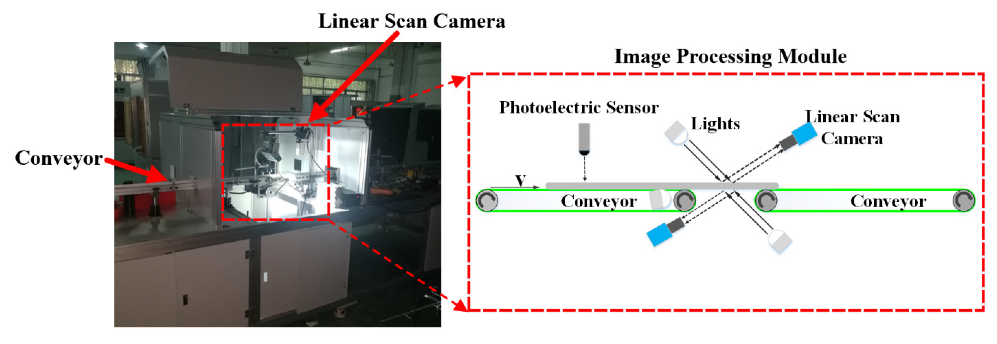
3.1. Experimental System

The experimental system consists of linear scan cameras, linear lights, industrial computer, conveyor, and other necessary mechanical parts (as seen in Figure 9). The linear scan camera is DALSA-LA-GM-02K08A, which has the resolution of 2048 × 1, a pixel size of 7.08 μm, and a max line rate of up to 52 K. The proposed algorithm was implemented in C++ using OpenCV library and ran on a computer with a i7-6700 CPU, 8G DDR memory.

In the experiment, the conveyor belt moved at a constant speed of 2 m/s, the flat aluminum tubes to be tested were placed on the conveyor belt one by one, and the photoelectric sensor was used to detect whether the flat tubes reached the camera imaging position. When defective products are detected, the follow-up mechanism will remove the flat tubes.

In this experiment, two different types of flat tube (namely type A and type B) were used to test the performance of the proposed method. These two kinds of tube have different length, width, height, and interval time, as seen in

Table 1. Parameters of Test Tubes.

Parameters	Type A	Type B
Length	800 mm	200 mm
Width	50 mm	10 mm
Height	2 mm	1 mm
Speed of Conveyor	2 m/s	2 m/s
Interval Time	500 ms	333 ms

. The flat tube samples were put one by one on the conveyor, so the “interval time” in Table 1 means the time between two flat tubes. In order to achieve real-time detection, the time duration of the algorithm should be less than the interval time.

For every type, 200 samples were used, in which there were 100 samples with no defects and another 100 samples with scratch defects. All the defects’ samples were labeled manually by quality inspectors of the manufacture factory.

3.2. Parameters Setting

In this proposed method, there are two parameters that may affect the algorithm performance, including the length of sub points set $length=2L+1$ (fitting curve length) used in Equation (1), and the total candidate number $N$ (sample number) used in Equation (6). In order to figure out how these two parameters influence the performance of the proposed method, two corresponding experiments were introduced.

The experimental results of the relation between curve length and location of the local maximums are shown in Figure 10. For the same input histogram image, when the length was small, the curvature curve was as chaotic as the histogram and many of false positions were detected. However, the local maximums were getting more and more obvious in the curvature curves as the length got larger. When the length was up to 151, the second peak that was detected in length 101/121/131 was not detected anymore. As a result, the best choice of the length should depend on the application requirements: if in the application the false positives are not allowed, then a larger length should be used, while in same applications if a small percentage of false positives are allowed, the middle range of the length (101/121/131) is better. In this work, the length is set to 131.

The sample number in Equation (6) indicates how many random control points will be used to generate the corresponding Bezier curves. In this experiment, random uniform distribution was used. General speaking, the more the sample number, the more accurate the fitting result, and also the more time that was consumed, but actually, when the sample number is larger than a certain number, the difference in accuracy is relatively small. As seen in Figure 11, there were some small differences of the fitting results between six different sample numbers (20, 40, 60, 80, 100, 120), but all of them can locate the local maximums correctly with very small position errors. It can be proved that, in a sample range of $N_w\times N_h$, where $N_w$ is the width of the sample area, and $N_h$ is the height of the area, if a control point falls within a 5 × 5 neighborhood centered on the correct control point position, and it is considered to be approximately correct, then the minimum sample number is $N\ge \frac{N_w\times N_h}{5\times 5}$. The detailed proof can be found in Section 2.4. According to this result, if $N_w=20$ and $N_h=20$, then the least sample number is $N=16$, which was well verified by the experiments. In this work, $N=60$ was used.

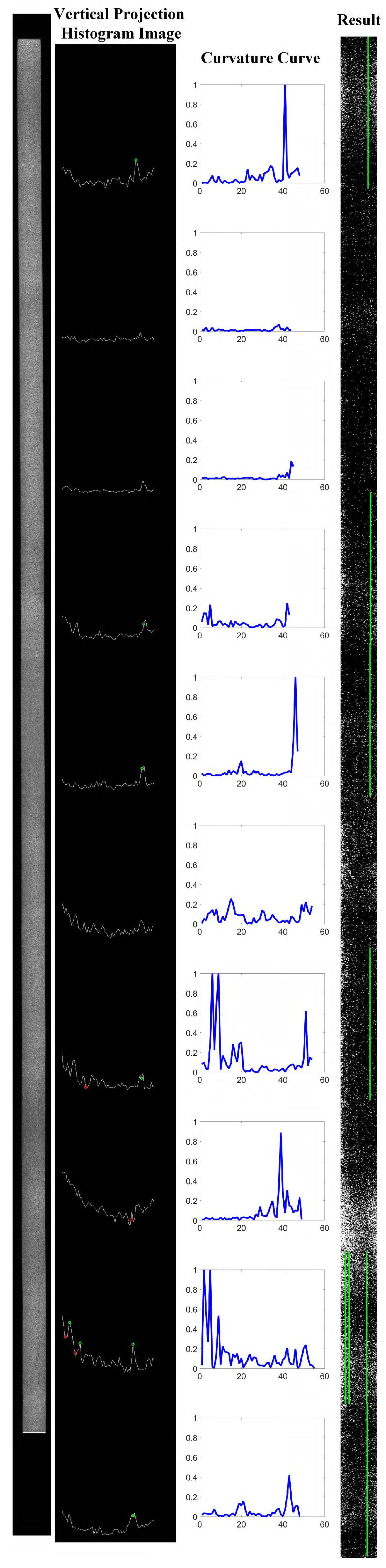
3.3. Experimental Results and Discussion

The experimental results can be seen in

Table 2. Experimental Results.

Results	Type A		Type B
	No Defects	With Defects	No Defects	With Defects
Total sample number	100	100	100	100
$N_{OK}$	93	2	95	1
$N_{NG}$	7	98	5	99
Time consuming/ms	459.32	478.24	87.65	98.31
FN/%	1%		0.5%
FP/%	3.5%		2.5%

. In the table, $N_{OK}$ means the number of samples that are detected as OK (no defect). For example, in column one, the number 93 means 93 out of 100 of “No Defects” in type A were detected as OK by our method, while $N_{NG}$ in the same column means 7 out of 100 of “No Defects” in type A were detected as NG (with defects) by our method.

FN means false negative, which means it should be positive (with defects), but the detection result of the algorithm is negative, while FP means false positive, which means it should be negative (no defects), but the result of the algorithm is positive. In the industrial application, FN is much more serious than FP. In our test, the FN is 1% and 0.5% using samples of type A and type B, respectively, while FP is 3.5% and 2.5%. From the results, we can find that there are still some cases that our method cannot detect correctly, and after a recheck of these samples, we found that these are truly “hard samples” that even experienced workers of the factory need to check very carefully from every possible observation angle. The total FN and FP results are at the same level as experienced works, while its efficiency is higher because it can work tirelessly.

The time duration of both type A and type B was less than the corresponding interval time in Table 1, which means the system can achieve real-time detection in different sizes of input flat tubes; furthermore, the time duration can be much less if a better computer is used in the future.

Some more detailed experimental results can be found in Figure 12, Figure 13, Figure 14 and Figure 15. In every image of the results, there are four images: the first one is the input test image, the second one is the result of vertical projection histogram images of 10 sections, the third one is the curvature curves based on the histogram image, and the last one is the detection result, in which the green line indicates the location of the scratches. The green circles in the histogram images are the detected local peaks of the histogram by our algorithm. It can be seen from the experimental results that, although the defects in some input images were very weak, and some were even difficult for people to distinguish, after the method proposed in this paper, the local peaks where the defects are located were highlighted, and the background noise where it was located was suppressed. Eventually, all the defects were detected effectively, and the locations of the defects were marked.

By analyzing and comparing the defects detected by the algorithm with the manually marked defects, it can be found that common and obvious surface defects both can be detected 100%, but when affected by the presence of volatile machine oil on the surface of some incoming flat tubes, the image characteristics were similar to the morphology of some of these surface scratch defects. Thus there will be a certain degree of misdetection, as shown in Figure 16. At the same time, for a small part of the detection of subtle scuffing defects, the algorithm did not detect them perfectly, that is, there was a certain degree of false negatives, but at the same time, it must be noted that the same missed detection can occur in this case, even for experienced workers.

4. Conclusions

This paper proposed a scratch detection system based on a cubic Bezier curve fitting using a linear scan camera in real-time under complex uncertain background noise. The key point of the proposed method involved using the Monte Carlo sampling method to calculate the best fitted cubic Bezier curves of every point in the vertical projection histogram curve, and the scratches were detected by finding the local peaks of curvature curve. In the experiment, a linear scan camera that captured the image of flat tubes on a moving speed of 2m/s was used to test the validity of the proposed method. The experimental results showed that the total FN and FP results are at the same level as experienced works, while its efficiency is higher because it can work tirelessly, which means it is possible to substitute the workers by our system in the future.

The experimental results of different fitting curve lengths showed that selection of this parameter was important to the algorithm performance. The selection should depend on application requirements, which means an adaptive selection of the fitting curve length will be an issue worthy of study in the future.

References

1. Chodankar, V.A.V.L.; Seetharamu, K.N. Improved effectiveness of a cryogenic counter-current parallel flow—Three fluid heat exchanger with three thermal communication due to Joule Thomson pressure drop. Int. J. Therm. Sci. 2022, 172, 107267. [Google Scholar] [CrossRef]
2. Yu, C.; Wang, Y.; Zhang, H.; Zeng, M.; Gao, B.; Fang, Z. Numerical investigation on turbulent thermal performance of parallel flow heat exchanger with a novel polyhedral longitudinal vortex generator in shell side. Int. J. Therm. Sci. 2021, 166, 106962. [Google Scholar] [CrossRef]
3. Abu-Hamdeh, N.H.; Salilih, E.M. Numerical modelling of a parallel flow heat exchanger with two-phase heat transfer process. Int. Commun. Heat Mass Transf. 2021, 120, 105005. [Google Scholar] [CrossRef]
4. Wang, Y.W.; Ni, Y.Q.; Wang, X. Real-time defect detection of high-speed train wheels by using Bayesian forecasting and dynamic model. Mech. Syst. Signal Process. 2020, 139, 106654. [Google Scholar] [CrossRef]
5. Horan, P.; Underhill, P.R.; Krause, T.W. Pulsed eddy current detection of cracks in F/A-18 inner wing spar without wing skin removal using Modified Principal Component Analysis. NDT E Int. 2013, 55, 21–27. [Google Scholar] [CrossRef]
6. Arjun, V.; Sasi, B.; Rao, B.P.C.; Mukhopadhyay, C.K.; Jayakumar, T. Optimisation of pulsed eddy current probe for detection of sub-surface defects in stainless steel plates. Sens. Actuators A Phys. 2015, 226, 69–75. [Google Scholar] [CrossRef]
7. Peng, J.; Tian, G.Y.; Wang, L.; Zhang, Y.; Li, K.; Gao, X. Investigation into eddy current pulsed thermography for rolling contact fatigue detection and characterization. NDT E Int. 2015, 74, 72–80. [Google Scholar] [CrossRef]
8. Huang, D.; Li, K.; Tian, G.Y.; Sunny, A.I.; Chen, X.; Tang, C.; Wu, J.; Zhang, H.; Zhao, A. Thermal pattern reconstruction of surface condition on freeform-surface using eddy current pulsed thermography. Sens. Actuators A Phys. 2016, 251, 248–257. [Google Scholar] [CrossRef]
9. Sunny, A.I.; Tian, G.Y.; Zhang, J.; Pal, M. Low frequency (LF) RFID sensors and selective transient feature extraction for corrosion characterisation. Sens. Actuators A Phys. 2016, 241, 34–43. [Google Scholar] [CrossRef] [Green Version]
10. Tehranchi, M.M.; Ranjbaran, M.; Eftekhari, H. Double core giant magneto-impedance sensors for the inspection of magnetic flux leakage from metal surface cracks. Sens. Actuators A Phys. 2011, 170, 55–61. [Google Scholar] [CrossRef]
11. Baek, I.; Cho, B.K.; Gadsden, S.A.; Eggleton, C.; Oh, M.; Mo, C.; Kim, M.S. A novel hyperspectral line-scan imaging method for whole surfaces of round shaped agricultural products. Biosyst. Eng. 2019, 188, 57–66. [Google Scholar] [CrossRef]
12. Zhang, X.-W.; Ding, Y.-Q.; Lv, Y.-Y.; Shi, A.-Y.; Liang, R.-Y. A vision inspection system for the surface defects of strongly reflected metal based on multi-class SVM. Expert Syst. Appl. 2011, 38, 5930–5939. [Google Scholar]
13. Song, K.; Yan, Y. A noise robust method based on completed local binary patterns for hot-rolled steel strip surface defects. Appl. Surf. Sci. 2013, 285, 858–864. [Google Scholar] [CrossRef]
14. Liu, X.; Xu, K.; Zhou, P.; Zhou, D.; Zhou, Y. Surface defect identification of aluminium strips with non-subsampled shearlet transform. Opt. Lasers Eng. 2020, 127, 105986. [Google Scholar] [CrossRef]
15. Li, J.; Su, Z.; Geng, J.; Yin, Y. Real-time Detection of Steel Strip Surface Defects Based on Improved YOLO Detection Network. IFAC-PapersOnLine 2018, 51, 76–81. [Google Scholar] [CrossRef]
16. He, Y.; Song, K.; Meng, Q.; Yan, Y. An End-to-End Steel Surface Defect Detection Approach via Fusing Multiple Hierarchical Features. IEEE Trans. Instrum. Meas. 2020, 69, 1493–1504. [Google Scholar] [CrossRef]
17. Huang, D.; Liao, S.; Sunny, A.I.; Yu, S. A novel automatic surface scratch defect detection for fluid-conveying tube of Coriolis mass flow-meter based on 2D-direction filter. Measurement 2018, 126, 332–341. [Google Scholar] [CrossRef]
18. Di, H.; Xu, K.; Zhou, P.; Zhou, D. Surface defect classification of steels with a new semi-supervised learning method. Opt. Lasers Eng. 2019, 117, 40–48. [Google Scholar] [CrossRef]
19. Zhang, D.; Song, K.; Xu, J.; He, Y.; Yan, Y. Unified detection method of aluminium profile surface defects: Common and rare defect categories. Opt. Lasers Eng. 2020, 126, 105936. [Google Scholar] [CrossRef]
20. Otsu, N. A Threshold Selection Method from Gray-Level Histograms. IEEE Trans. Syst. Man Cybern. 1979, 9, 62–66. [Google Scholar] [CrossRef] [Green Version]
21. Saleem, N.; Agwu, I.K.; Ishtiaq, U.; Radenović, S. Strong Convergence Theorems for a Finite Family of Enriched Strictly Pseudocontractive Mappings and Φ T-Enriched Lipschitizian Mappings Using a New Modified Mixed-Type Ishikawa Iteration Scheme with Error. Symmetry 2022, 14, 1032. [Google Scholar] [CrossRef]
22. Saleem, N.; Isık, H.; Khaleeq, S.; Park, C. Interpolative Ciric-Reich-Rus-type best proximity point results with applications. AIMS Math. 2022, 7, 9731–9747. [Google Scholar] [CrossRef]
Figure 1. Microchannel Aluminum Flat Tube and Parallel Flow Heat Exchanger.
Applsci 12 06049 g001
Figure 2. Examples of surface defects.
Applsci 12 06049 g002
Figure 3. Segmentation of the Input Image.
Applsci 12 06049 g003
Figure 4. Overview of the proposed method. (a) The section 5 of input image. (b) The result of preprocessing. (c) The vertical projection histogram curve. (d) The curvature curve.
Applsci 12 06049 g004
Figure 5. Sub points set centered at C P m .
Applsci 12 06049 g005
Figure 6. Cubic Bezier Curve.
Applsci 12 06049 g006
Figure 7. Distribution of control points.
Applsci 12 06049 g007
Figure 8. The result of cubic Bezier curve fitting. The green circle in the vertical projection histogram image represents the local peak detected by the proposed method.
Applsci 12 06049 g008
Figure 9. The detection and experimental system.
Applsci 12 06049 g009
Figure 10. Bezier curve fitting and curvature results using different sub curve length.
Applsci 12 06049 g010
Figure 11. Bezier curve fitting results using different sample number.
Applsci 12 06049 g011
Figure 12. Result 1. The green circles represent local maximums, red circles represent local valleys, and the green lines represent the detected scratches.
Applsci 12 06049 g012
Figure 13. Result 2. The green circles represent local maximums, red circles represent local valleys, and the green lines represent the detected scratches.
Applsci 12 06049 g013
Figure 14. Result 3. The green circles represent local maximums, red circles represent local valleys, and the green lines represent the detected scratches.
Applsci 12 06049 g014
Figure 15. Result 4. The green circles represent local maximums, red circles represent local valleys, and the green lines represent the detected scratches.
Applsci 12 06049 g015
Figure 16. Interference of oil to normal flat tube.
Applsci 12 06049 g016