A Spike Neural Network Model for Lateral Suppression of Spike-Timing-Dependent Plasticity with Adaptive Threshold

Abstract

Aiming at the practical constraints of high resource occupancy and complex calculations in the existing Spike Neural Network (SNN) image classification model, in order to seek a more lightweight and efficient machine vision solution, this paper proposes an adaptive threshold Spike Neural Network (SNN) model of lateral inhibition of Spike-Timing-Dependent Plasticity (STDP). The conversion from grayscale image to pulse sequence is completed by convolution normalization and first pulse time coding. The network self-classification is realized by combining the classical Spike-Timing-Dependent Plasticity algorithm (STDP) and lateral suppression algorithm. The occurrence of overfitting is effectively suppressed by introducing an adaptive threshold. The experimental results on the MNIST data set show that compared with the traditional SNN classification model, the complexity of the weight update algorithm is reduced from O(n²) to O(1), and the accuracy rate can still remain stable at about 96%. The provided model is conducive to the migration of software algorithms to the bottom layer of the hardware platform, and can provide a reference for the realization of edge computing solutions for small intelligent hardware terminals with high efficiency and low power consumption.

1. Introduction

Spiking Neural Networks (SNN) is the third generation neural network model, derived from the biological neural network [1,2]. SNN is the information transfer process between the neurons of the organism. It is fully biologically interpretable, has two advantages of high performance and low power consumption, and has increasingly become a research focus in the field of brain-like computing, especially in the direction of machine vision [3]. The traditional Artificial Neural Network (ANN) encodes neural information through the frequency of pulse firing [4], and its learning algorithm minimizes the error function by adjusting the synaptic strength. Gao [5] detects the fatigue driving problem through EEG-based Spatial Temporal Convolutional Neural Network; Michielli [6] proposes a method for classifying EEG sleep data by state based on Cascaded LSTM Recurrent Neural Network; Mohammadi [7] proposed an EEG signal classifier for depression diagnosis, called FFNN (Fuzzy Function based on Neural Network). Although the traditional ANN classification method has provided great help for EEG researchers, it has a strong dependence on feature extraction. The choice of feature extraction method will have a great impact on the classification accuracy, so it takes a lot of time and energy to choose a suitable feature extraction method. The iteration of ANN relies on the error BP (Back-Propagation) algorithm, which has relatively high requirements on the computing power of the platform. SNN avoids the time and energy spent in manual data processing and selection of feature extraction methods. Its iteration does not depend on the BP algorithm, which greatly reduces the requirements for the computing power of the platform, which is conducive to the deployment of algorithms in distributed systems and can solve online learning problems in other scenarios such as edge computing. Kasabov et al. [8] built a development environment called NeuCube based on SNN, which can be used for the research of brain-like artificial intelligence. Compared with traditional machine learning methods, NeuCube has higher classification accuracy for brain spatiotemporal data, and the platform calculation amount is greatly reduced than that of traditional machine learning methods [9,10]. Therefore, SNN has attracted a lot of attention from researchers and are generally regarded as a lightweight, energy-efficient hardware-friendly image recognition solution.

In recent years, the Spike-Time-Dependent-Plasticity (STDP) algorithm has gradually become one of the mainstream learning algorithms for SNN models due to its profound physiological basis and efficient regulatory mechanism, and has been successfully applied to fields such as field programmable on hardware terminals such as logic gate arrays and application-specific integrated circuits. In particular, Kheradpisheh et al. [11,12] extracted the input features through the sorting coding method and the simplified STDP algorithm, and then used the Support Vector Machine (SVM) to complete the output classification, and finally obtained the Face/Moto subset of the Caltech dataset. The accuracy rate of 99.1%; Lee et al. [13,14] used Poisson coding and fully connected output structure based on the existing STDP algorithm to realize the neuron model as a network node, the self-classification of the intermediate SNN, and for the Face/Moto dataset. The classification accuracy can reach 97.6%. In order to further improve the classification performance of the STDP algorithm on SNN, Zheng et al. [15] extended the BP algorithm to the supervised learning of the pulse sequence pattern of the STDP algorithm, combined with the stochastic gradient descent method for training, and achieved 97.8% on the MNIST dataset. On the basis of literature research, Mozafari et al. [16,17] modified the weight change results of the STDP algorithm twice by introducing reinforcement learning, which overcomes the dependence of the original network structure on external classifiers such as SVM. The classification accuracy on the dataset reaches 98.9%.

To sum up, researchers have made a lot of improvements in the adaptation of STDP algorithm and SNN model in their respective sub-fields, but in the face of constraints such as resource limitations and computing power bottlenecks that exist widely in practical application scenarios. There is still room for optimization. Diehl et al. [18] constructed an SNN model, which included 28 × 28 neurons in the input layer, processing layer neurons and corresponding inhibitory layer neurons in second layer, synapses are regulated by the STDP mechanism. It is found that the accuracy of this model on MNIST dataset can reach 95%. Though this model achieved better classification performance, it occupied more hardware resources and led to higher computing power consumption [19,20,21]. Software algorithms are the core of neuromorphic computing, and hardware devices are software dependent [22,23]. As the carrier of operation, the two are inseparable. The one-sided pursuit of software performance is mostly the overdraft of hardware computing power [24,25,26,27]. Especially with the rise of heterogeneous computing software platforms, software and hardware co-design has gradually become one of the commanding heights of technological competition [28,29,30]. Accordingly, this paper proposes a spiking neural network model for lateral suppression of STDP with adaptive threshold. The conversion from grayscale image to pulse sequence is completed by convolution normalization and first pulse time coding. The network self-classification is realized by combining the classical pulse time-dependent plasticity algorithm (STDP) and lateral suppression algorithm. The introduction of adaptive thresholds ensures the sparsity of pulse delivery and the specificity of learning features, effectively suppresses the occurrence of over-fitting, and facilitates the migration of software algorithms to the bottom layer of the hardware platform, which can be a high-efficiency, low-power, small-sized and intelligent provide reference for the realization of edge computing solutions of hardware terminals.

2. Network Model

The STDP impulse neural network model based on the adaptive threshold uses the Leaky Integrate-and-Fire (LIF) neuron model as the network node, and the intermediate synapse information is transmitted in the form of pulses. Its basic structure is shown in Figure 1. As shown, it can be divided into pulse coding layer, neural network layer and classification layer in turn. The pulse coding layer encodes each pixel of the image into a pulse whenever the image needs to be classified. After the image is encoded into a pulse, it is trained by two neural network layers. The first neural network layer contains 100 neurons, and the second neural network layer contains 20 neurons. The neural network layer includes two layers of nerves. Between each layer of neurons, the weights of neuron connections are updated through the STDP algorithm, and the neurons of the same layer are laterally inhibited; the classification layer classifies the signals processed by the neural network layer.

2.1. Pulse Coding

The spiking neural network simulates biological neurons receiving pulse sequences as input. In order to design an efficient SNN system, it is necessary to adopt an appropriate pulse coding strategy to encode sample data or external stimuli into discrete pulse sequences. The researchers draw on the coding mechanism of biological neurons for specific stimulation signals, and mainly provide two types of pulse coding methods: coding based on pulse frequency and coding based on pulse time. Frequency coding considers that information is contained in the firing frequency of the pulse. Compared with pulse frequency coding, the algorithm based on pulse time coding assumes that the distinguishing characteristic information is contained in the specific pulse firing time rather than the signal amplitude or pulse density. With stronger biological authenticity and computational efficiency. Considering the generalization ability and applicability of the coding algorithm, this paper converts frame-based static image data into time pulse sequence data processing, and improves it according to practical application and data knowledge.

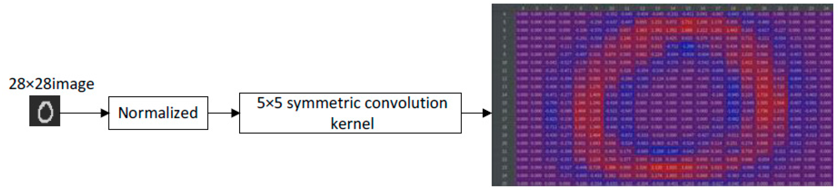
Due to the difference in size and format between the input images, it needs to be preprocessed first. This paper normalizes the original image uniformly, multiplies it by the symmetrical convolution kernel, and blurs it into a 28 × 28 grayscale image. The pixel value of the image is in the range of [−2, −2], while retaining the input characteristics of the image, such as Figure 2 shows the blurring process performed on the handwritten number “0” with a pixel of 28 × 28.

The input pulse of the network model is represented by time encoding, and a single neuron can only emit a single pulse, which then acts on the post-neuron through weighted connections. In order to convert the input image into the input pulse sequence, the gray value of each pixel needs to be encoded. Time-to-First-Spike (TTFS) coding is a commonly used linear time coding method for grayscale images. The higher the grayscale value of a pixel, the more obvious the input feature is, and the corresponding pulse will be sent earlier. Lower grayscale values will emit later. That is, the pixels whose pixel values are in the range of [−2, −2] after convolution are linearly mapped to the time scale of 0-T in turn. In order to ensure that the initial pulses of all input layers can have a chance to be transmitted to the output layer, the timing of the initial pulses should satisfy.

$$t=\left|\frac{P_{\max }-P}{P_{\max }-P_{\min }}\cdot (T-L+1)\right|$$

(1)

In the formula: P is the gray value corresponding to the input pixel, P_max and P_min are the maximum and minimum values, respectively; T is the processing cycle of a single input image; L is the number of layers of the network model. The result of (1) is rounded down to make it discretized, so as to conform to the discrete-time expression form of the pulse sequence. Whenever a pulse is sent from the input layer at a certain time t, the output layer can respond at least at time t + L − 1, which ensures the continuous transmission of the input features within the period T. Apply the Formula (1) to calculate the time t for each pixel to emit a pulse. 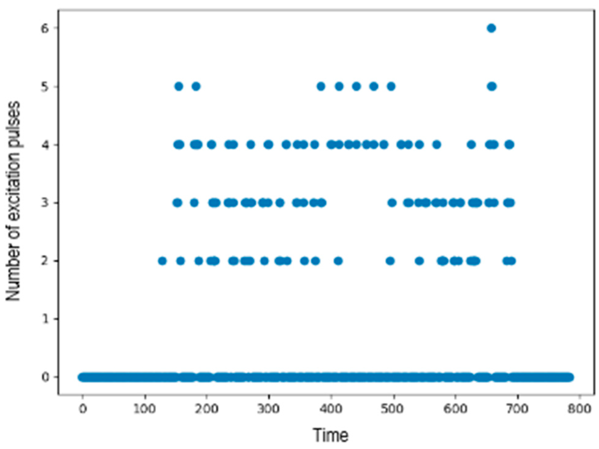During the entire period T, the corresponding pixel generates a pulse every time t. TTFS coding performs discrete linear coding on the gray value for T periods, so that the pixel values in the range of [−2, −2] are projected into the period T, ensuring that most pixels generate pulses within the discrete T discrete time periods. As shown in Figure 3, the number of excitation pulses of the 784 pixels in the picture “0” in the period T, the average number of pulses in the picture is 4.33 through statistical calculation.

2.2. LIF Model with Adaptive Threshold to Update the Electric Potential of Neurons

2.2.1. Neuron Model

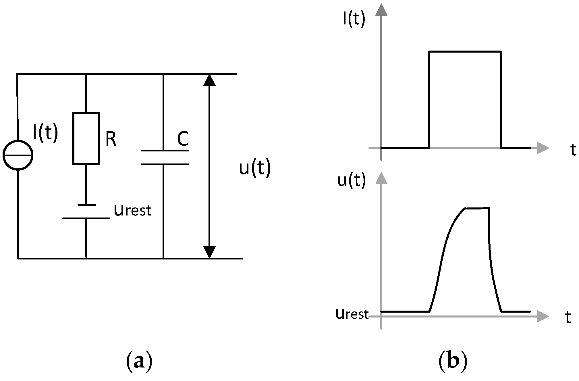
In the LIF model, the cell membrane continuously exchanges ions inside and outside the membrane. When there is only one input, the voltage will leak and slowly fall back to a resting state. The LIF model believes that it first drops below the resting membrane potential, and then rises to the resting potential. This model equates neurons as an RC circuit composed of capacitors (representing neuron cell membranes) and resistors (representing ion channels), as shown in Figure 4a.

Figure 4b depicts the relationship between the neuron’s membrane potential u and the input current I. The transformation process of membrane potential u is described by the following first-order differential equation:

$$I_i(t)=\frac{u_i(t)-u_{reset}}{R_m}+C_m\frac{d{u}_i(t)}{dt}$$

(2)

The standard LIF differential model can be obtained by deforming:

$$\begin{array}{l}{\tau }_{mem}\frac{d{u}_i(t)}{dt}=-(u_i(t)-u_{reset})+R_m{I}_i(t),u_i(t)<u_{th}\\ u_i(t)=u_{reset},u_i(t)\ge u_{th}\end{array}$$

(3)

where $u_i(t)$ represents the cell membrane potential of the neuron $i$ at time t, $u_{reset}$ represents the resting membrane voltage, and ${\tau }_{mem}=R_m{C}_m$ is the cell membrane time constant. When the cell membrane potential $u_i$ exceeds the threshold $u_{th}$, the neuron emits pulses and resets to $u_{reset}$.

2.2.2. Adaptive Threshold

In unsupervised learning, because the activation amount of each picture mode is different, as shown in

Table 1. Average Number of Pulses.

Image	Average Number
“0”	4.33
“1”	2.667
“2”	5.667
“3”	4.667
“4”	5
“5”	4
“6”	5
“7”	3
“8”	4.667
“9”	4.33

, it is difficult to train a network. Modes with higher activation tend to win in competitive learning, eclipsing other modes. Therefore, the introduction of variable thresholds reduces them all to the same level, avoiding that the image mode with a high degree of activation always wins. The threshold of each mode is calculated based on the number of activations it contains. The higher the number of activations, the higher the threshold, correspondingly, the lower the number of activations, the lower the threshold.

In this paper, the threshold of each picture is different, and it is updated in real time according to the picture. As shown in Figure 3, considering many zero pulses, the maximum value of the number of pulses does not exceed 10. The tail-cut average method will reduce the number of pulses too low, so the calculation of the threshold adopts the arithmetic average method. Calculate the number of pulses of all pixels in each time step for the picture, accumulate in the entire time period, and finally take the arithmetic average value as the threshold of the picture. Different pictures have different thresholds to adapt to different activation levels of different pictures to avoid excessive activation.

2.3. STDP Algorithm

The important part where neurons come into contact with each other is called synapse, which can be used to transmit information. Among them, presynaptic neurons emit information and post-synaptic neurons receive information. The property of a synapse to continuously change and adjust itself to suit the needs of the body under various stimuli and influences is called synaptic plasticity. The STDP algorithm establishes associations between neural stimuli and modulates synaptic connection weights. Its weight learning mechanism can be expressed as,

$$\Delta w={\displaystyle \sum _{t_{pre}}{\displaystyle \sum _{t_{post}}w(t_{post}-t_{pre})}}$$

(4)

$t_{post}$ represents the time when a post-synaptic neuron generates a pulse, and $t_{pre}$ represents the time when a pre-synaptic neuron generates a pulse. The regulation of synaptic connection weights is specifically described by STDP rules, if pre-synaptic neurons are stimulated before post-synaptic neurons, it will lead to long-term potentiation of synapses (LTP), that is, the weight of the connection between the synapses of two neurons will increase, otherwise it will lead to long-term depression (LTD) of the synapse, that is, the weight of the connection between the synapses of two neurons will decrease. The conventional STDP time function is as follows:

$$\begin{array}{l}w(\Delta t)=A_{+}\exp (\frac{\Delta t}{{\tau }_{+}}),\Delta t\ge 0\\ w(\Delta t)=A_{-}\exp (\frac{\Delta t}{{\tau }_{-}}),\Delta t<0\end{array}$$

(5)

Among them, $\Delta t$ represents the time when the post-synaptic neuron generates pulses, $A_{+}$ and $A_{-}$ represent the range of weight adjustment, ${\tau }_{+}$ and ${\tau }_{-}$ represent the constant of different neuron models.

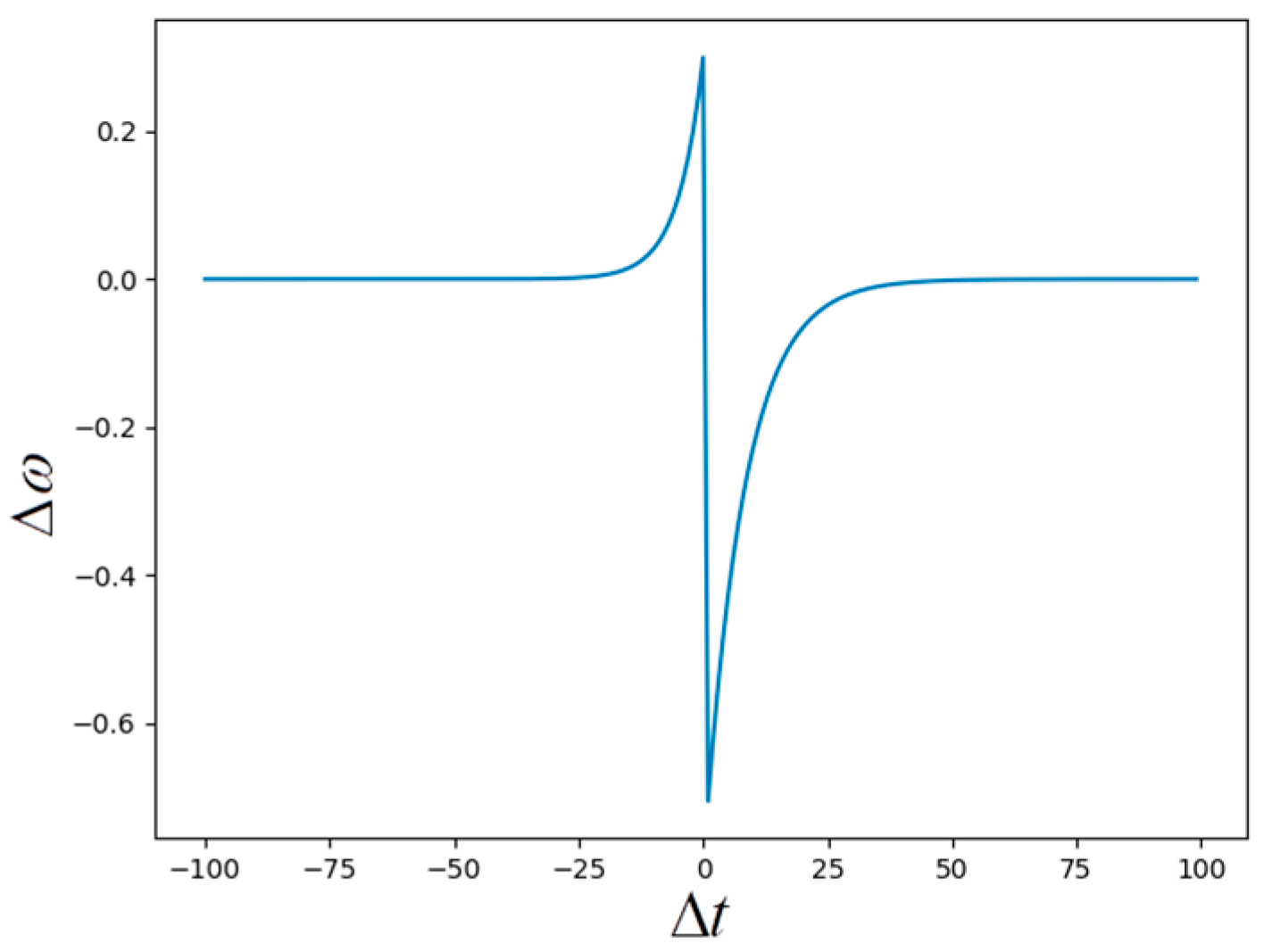
The parameter values in the STDP algorithm are shown in

Table 2. Learning Parameters of STDP.

Parameters	Values
$t_{pre}$	20
$t_{post}$	0
$A_{+}$	0.8
$A_{-}$	0.3
${\tau }_{+}$	8
${\tau }_{-}$	5

, and the STDP algorithm curve chart obtained under the parameters is shown in Figure 5. It can be seen from the figure that when $\Delta t<0$ there is a causal connection between the pre-neuron and the post-neuron, the synapse weight increment increases exponentially, and the shorter the pulse time interval is, the closer the connection is, and the more the corresponding synapse weight increases. When $\Delta t\ge 0$ there is an inverse causal connection between the front and back neurons, and the weight increment decreases exponentially, and the shorter the time difference, the more the weight decreases.

2.4. Lateral Inhibition Mechanism

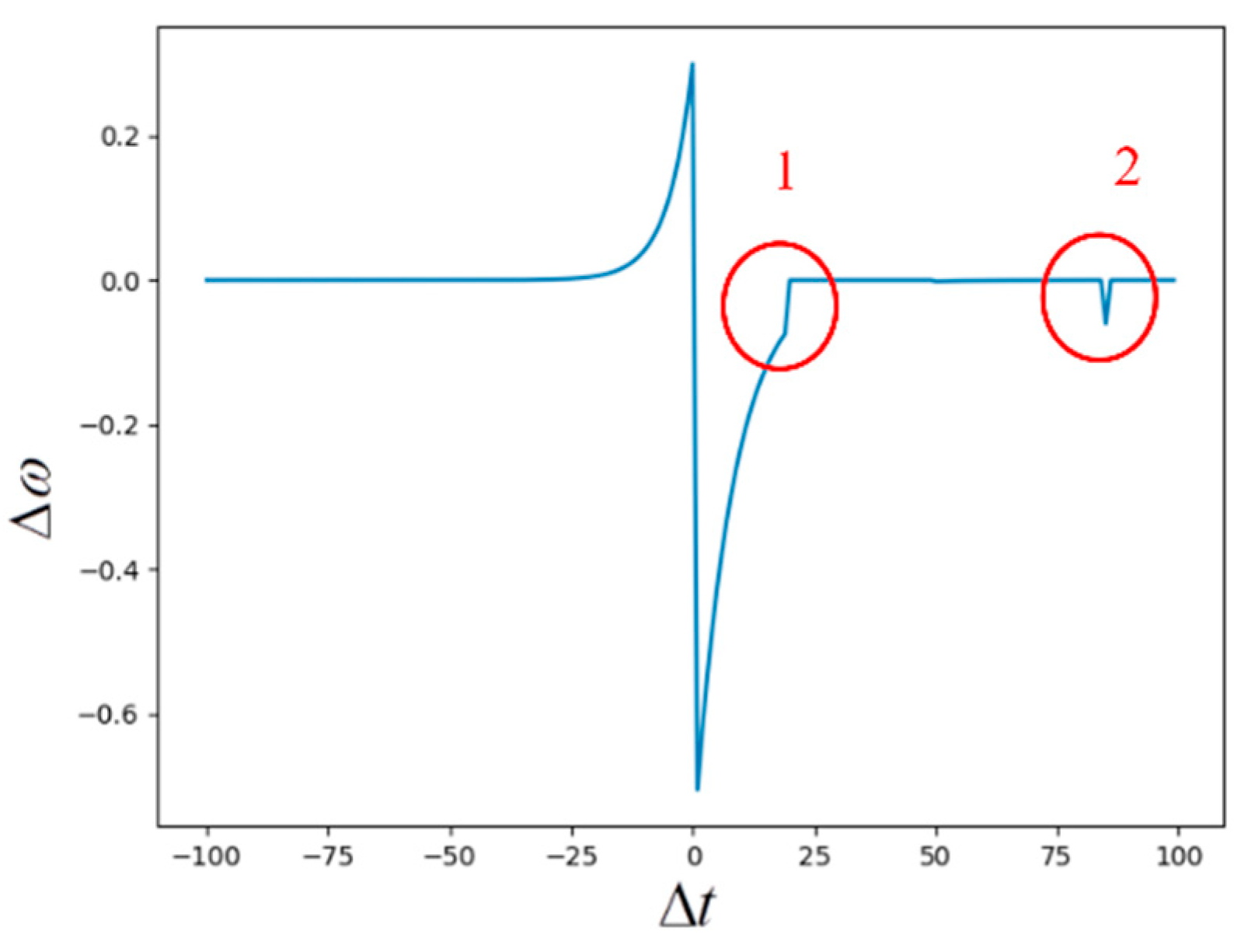
In order to make the excited neurons more prominent, this paper proposes a lateral inhibition algorithm. Lateral inhibition is to allow excited neurons to inhibit other neurons in the same layer, that is, to reduce the activity of neighboring neurons, so that the action potential cannot spread from the excited neuron to the neighboring neurons in the lateral direction. First, determine whether there is a neuron excitation pulse. In some cases, subtract the lateral inhibition attenuation value (value −0.06) from the weight of the neighbor neuron to reduce its weight. The red circle in Figure 6 is the excited neuron that causes the neighbor neuron to inhibit laterally. 1 is to accelerate the attenuation of the neighbor neuron’s weight, and 2 is where the neuron’s increment is zero, and the attenuation does not satisfy the STDP algorithm, so it is restored to zero.

3. Experimental Verification and Analysis

The experimental environment of this article is: Ubuntu19 operating system, 32 G memory, Inter^® Core TM i5-5200U CPU 2.20 Hz, 2 GTX 1080 Ti graphics cards. Use Python2.7.5 as the environment to build the SNN model for Lateral Suppression of STDP with Adaptive Threshold, and conduct verification experiments on the MNIST data set. The network parameters used in the experiment are shown in

Table 3. Parameters of SNN Model Network.

Parameters	Values
Time Step	200
Integration Time	0.005
Resting Voltage	0
Threshold Voltage	variable
Time Constant of Cell membrane	0.05

. Take the training data of the MNIST data set, and iterate it in the SNN model 1000 times to obtain the classification of numbers 0–9, test the classification of the test data of the MNIST data set, and use the correct rate of the classification of the test data as the performance evaluation index of the model. At the same time, record the accuracy of the test data set for reference.

All synapses connected to neurons in the output layer, if scaled to appropriate values and rearranged in the form of images, will describe the pattern that the neuron has learned and how to distinguish the pattern. After training the network with the MNIST data set, zoom all the weights of the neurons connected to the output layer, enlarge the weights to form a 28 × 28 image, and obtain a gray-scale neuron, which can more intuitively see the algorithm classification effect. 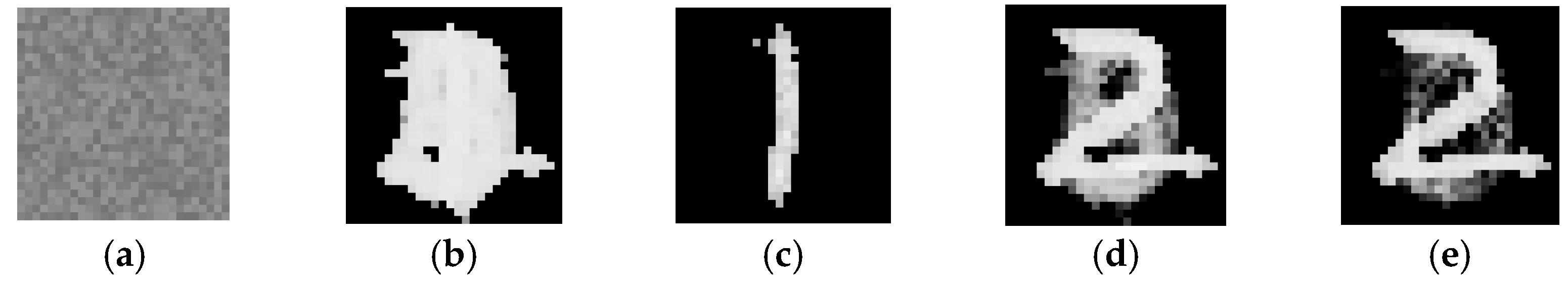Figure 7 is a comparison diagram of pulse thresholds, and Figure 8 is a corresponding reconstruction diagram of weights. The red line in Figure 7 is the threshold, the blue line is the number of pulses, and Figure 7a,b is the case of a fixed threshold. In Figure 7a, the threshold is too high, resulting in no pulses reaching the threshold, and the result becomes noise as shown in Figure 8a; in Figure 7b, the threshold is too low, causing the number of pulses to be too high, and there are too many pulses reaching the threshold. The result will be as shown in Figure 8b, the contours of the displayed digits are recognized, but the specific digits are not recognized; Figure 7c–e uses a variable threshold, and different thresholds are used for different pictures to avoid the occurrence of excessively high or low pulse numbers such as Figure 7a,b. Figure 7d does not add the lateral suppression algorithm. It is seen that digital ghosting appears in Figure 8d. The lateral suppression algorithm is used in Figure 7e. The number of pulses that exceed the threshold is further reduced, and the ghosting is also reduced a lot, which is much clearer than Figure 8d.

Since the traditional SNN model has a fixed threshold, the final result is prone to noise or ghosting problems. The threshold is changed into an adaptive threshold, and the variable threshold is adapted to different pictures, avoiding too many or too few pulses that exceed the threshold. At the same time, adding a lateral suppression algorithm can greatly reduce the ghost phenomenon.

Table 4. Algorithm Comparison.

Network Model	Learning Algorithm	Classification Accuracy (%)
SNN	STDP with Fixed Threshold	88.5
SNN	STDP with Adaptive Threshold	95.4
SNN	SNN with Adaptive Threshold Lateral Suppression	96.6

shows the results of six comparative experiments. The results show that compared with the traditional SNN model based on the fully connected structure, the recognition effect of the SNN model with adaptive threshold can be improved to a certain extent. At the same time, the SNN model fused with the lateral suppression algorithm has achieved accuracy that competes with the traditional SNN network model in the EEG recognition task.

In this paper, the scheduling method based on the discretized time domain greatly simplifies the pulse conversion and weight learning process: On the one hand, the pulse mode is limited to T = 200 through TTFS encoding. Compared to the sort encoding, the compression rate has reached 200/256 × 100% = 78.125%. On the other hand, discretizing the pulse sequence interval, which optimize the calculation process of weight update, reduces the complexity from O(n²) to O(1) compared with the classic continuous STDP algorithm. At the same time, this paper introduces a lateral suppression mechanism in the network iteration process to further ensure the sparsity of pulse delivery and the specificity of learning features, which reduce network complexity and training calculations. In addition, the introduction of adaptive thresholds also enables the model to suppress the occurrence of overfitting under limited resources without resorting to additional dynamic learning rates and random inactivation schemes. Compared with SNN model with other algorithm, classification accuracy of the SNN model fused with the lateral suppression algorithm is 96.6. Therefore, the model proposed in this paper can effectively reduce occupancy while ensuring good classification performance, which is more suitable for the realization of edge computing solutions of small intelligent hardware systems with high efficiency and low power consumption.

4. Conclusions

In order to solve the practical constraints such as high resource consumption and complex operation in the existing SNN image classification model, this paper proposes a spiking neural network model with adaptive threshold lateral suppression STDP, and obtains good classification on the MNIST dataset. The experimental results show that, compared with the traditional SNN classification model, this model has the following advantages: (1) The release and transmission of the pulse sequence adopts the discrete-time scheduling scheme, and the TTFS coding strategy simplifies the learning of the pulse pattern and weight, compared with the classical continuous STDP algorithm, the complexity is reduced from O(n²) to O(1); (2) The introduction of adaptive threshold ensures the sparsity of pulse transmission and the specificity of learning features, and effectively suppresses the occurrence of overfitting; (3) Combining the lateral suppression mechanism with the classic STDP algorithm realizes network self-classification without the need for additional classifier; (4) It occupies less network resources, has low model complexity, but classification accuracy is 96.6, superior to SNN models of other algorithms. These features are conducive to the realization of edge computing solutions for small intelligent hardware terminals with high efficiency and low power consumption.