A Grasshopper Plugin for Finite Element Analysis with Solid Elements and Its Application on Gridshell Nodes

Abstract

Linking architectural models to structural analyses can be demanding and time-consuming, especially when the architectural models cannot be accurately analysed using readily available one- or two-dimensional finite elements. This paper presents a tool for finite element analysis using solid elements developed as a plugin for Grasshopper 3D^® that enables designers to include analyses of complex objects within the same software as the design exploration. A benchmark using the tool on a cantilever beam is compared with both ANSYS^® and the theoretical solution, before the versatility of the tool is demonstrated by analyzing the metal part in timber gridshell nodes. The results were satisfying and the tool can prove especially useful for early phase design and collaboration between diciplines.

1. Introduction

Gridshells are shells where the structural members form a grid of linear elements rather than a continuous surface. Nodes are essential parts of a gridshell regarding structural performance, assembly and visual appearance. Due to the many decisions to be made when designing gridshells, including global shape, topology, cross-sections, material selection and node designs, detailed structural analysis of gridshell nodes is often left to later stages of the project. Getting feedback on the structural performance of gridshell nodes is inefficient due to software changes and geometry conversion, and it is hard to find tools that support early integration between architectural design and structural design. This work aims to develop a tool for finite element analysis (FEA) in Grasshopper 3D^®. The tool allows the designers to analyse the structural performance of gridshell nodes with volumetric analysis within the same software used for architectural design. An important feature of the tool is the possibility to automatically transform the architectural model into a structural analytical model through the volumetric meshing of geometries. The tool is evaluated using a benchmark and tested on geometries for the metal part of four gridshell nodes. Although the main focus of this article has been to establish the tool and the methodology applied on gridshell nodes, the tool can be useful in other applications.

2. Background

2.1. Gridshells

Gridshells, like other shell structures, are inherently material-efficient structures. Recent development in digital design tools has made gridshells more accessible amongst architects and engineers, with architects as drivers for interesting shapes and architectural concepts. Engineers are developing new methods for form-finding and analyses of gridshells.

In recent years, the Conceptual Structural Design Group at NTNU (CSDG) has been investigating conceptual design in the collaboration between architects and structural engineers, focusing on gridshells, resulting in both built prototypes and new design tools. In 2016 a temporary pavilion called Printshell was realised for a local festival in Trondheim. It had a footprint of 6 × 6 m and a height of 3 m. It was built from members of 48 × 48 mm of C24 spruce with standardised cuts at the ends and unique lengths. The ends of members were produced in the workshop with saw tables and were connected to 51 unique nodes produced with 3D-printing, hence the name Printshell. The nodes should distribute the forces between the members. As the nodes would be highly visible in the structure, it was essential to be able to visualise the geometries as precise as possible. Manufacture and analysis of the nodes was the key issue and focus of the project.

A parametric model was used to define the geometries for the nodes. The design workflow also included a connection between global and local modelling of the gridshell. The global model evaluated the overall structural performance, representing the gridshell members (beams) as the lines and nodes as the points. The global model enables the designer to preview the volumetric representation of the model. The local model included detailed node geometries. The global model and local geometry generation were done in a parametric environment using Rhinoceros^® and Grasshopper 3D^® [1], with the global structural analysis made in Karamba3D^® [2]. The local analysis on behavior of the nodes was made in ANSYS^® [3]. The design of relatively small elements cannot be done on the global model with readily available one- and two-dimensional finite elements. Therefore a Finite element analysis (FEA) with volumetric finite elements was deemed necessary for the analysis. However, the volumetric analysis was a computationally heavy and slow procedure, demanding changes between software and geometry conversion. The most crucial nodes were exported to ANSYS from Rhinoceros and analysed individually, with little options for automation. 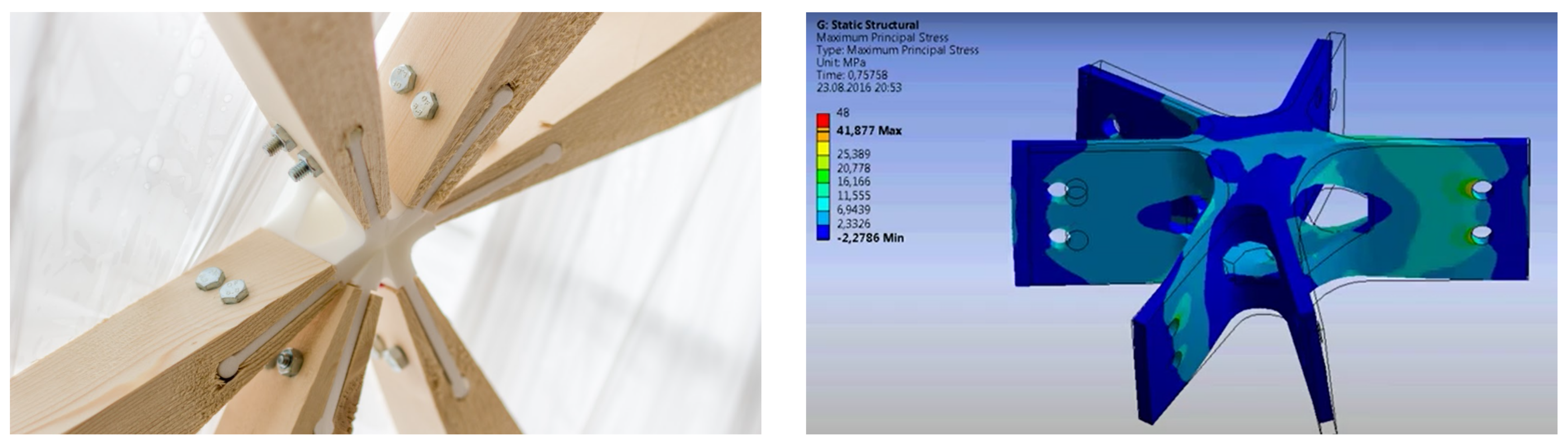Figure 1 shows one of the prindshell nodes, manufactured with 3D-printing, and an example of a node analysis in ANSYS.

2.2. Gridshell Nodes

Gridshell nodes have three main functions. First, they ensure structural integrity by transferring forces between the members; second, they play a key role in the assembly and prefabrication of a gridshell; lastly, they accommodate the small geometry changes between the connecting members. In addition, they can serve as visible objects that enhance the architectural concept.

Gridshells, like other shells, transfer forces primarily through in-plane membrane forces, which in gridshells are subjected to the members as axial forces. Although this enables efficient material usage, the slenderness makes shell structures subjected to compression forces prone to buckling and stability issues. In gridshells, the nodes are an integral part of the structural system. An assumption that these are rigidly connected to all the adjoining members is both an unrealistic and unconservative estimate. Rigid connections imply a complete transmission of bending moments between members and nodes, which causes the analytical model to be significantly stiffer than the actual system. Rigid connections are only possible in practice if all members are welded to the node. In addition, small gaps and imperfections from production allow for small node movements.

Modelling connections as either pinned or rigid is common in almost all practical finite element analyses. After extracting the forces in the node, a connection with the appropriate number of fasteners to withstand the internal forces is selected. By using a more realistic node stiffness based on the actual properties of the connector, the global behaviour of the system will be altered. For larger buildings and structures, the cost of the extra analysis done by the engineer is unfeasible compared to the price of some additional bolts and welds. However, for gridshells, where the form follows the forces, the advantage of accurate accounting for node rigidity is significant. A recent study by Lara-Bocanegra et al. demonstrates this importance on an elastic timber gridshell by comparing the deflections of a full-scale model to those of a numerical analysis [4]. Without considering the joints’ rigidity, the analytical model underestimates the deflections and fails to capture the gridshell’s physical behaviour. Therefore, joint rigidity is an important factor when evaluating gridshells as using pinned joints in the evaluation often leads to unstable structures, and rigid joints could result in too unconservative estimates. Several studies report this, including [5,6,7].

Nodes are also often reported as the most expensive parts in realising gridshells [8,9,10]. Nodes are thus both crucial for the structural integrity and the final cost of a gridshell; however, recent studies by the authors have shown that gridshell nodes are not a pronounced priority in recent research on gridshells [11]. When selecting nodes for a steel and aluminium gridshell, manufacturing companies can provide a set of pre-accepted solutions. For timber gridshells, the nodes are typically developed for each project. Analyses of gridshell nodes are typically done using solid elements as seen in the recent studies by Castriotto et al. [12] and Seifi et al. [7]. Like in the Printshell project presented in Section 2.1, the analyses require exporting to separate tools for performing the meshing and analyses. Structural or mechanical engineers often drive the design of nodes. Harris et al. describe [13] how timber engineers designed the nodes for The Pods sports academy B&K Structures with Westmucket and Hawkes (structural consultants) as sub-contractors for the detailing of the nodes.

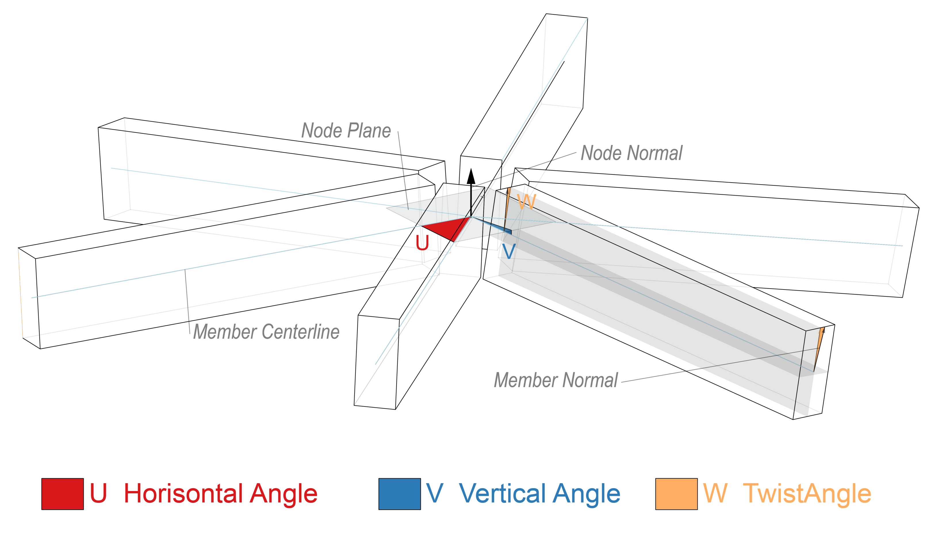
The geometry deviations between the members’- and the node’s plane can be described with three angles, often referred to as the U-, V-, and W-angles [14]. Figure 2 illustrates these three angles. The U-angle represents the horizontal angle, meaning the angle between two members in the node plane, the vertical angle, V, represents the vertical kink between the normal direction of two nodes at each end of a member, and the twist angle, W, represents the twist between the same normal directions. In general, the nodes need high precision in manufacturing to accommodate these angles.

To summarise, gridshell nodes are crucial for both the structural performance and costs of a gridshell, especially in timber gridshells. The main challenge in designing gridshell nodes is the need for analyses with inefficient software changes and geometry conversions. One way to solve this challenge is to include volumetric analyses within the same environment used for the architectural design of the gridshell. With the evaluation of node geometries within the same design environment, the designers, architects and engineers could more easily understand the implications of specific node designs at the global scale and include the design of the nodes as visible objects in the design concept.

2.3. Architectural versus Analytical Models

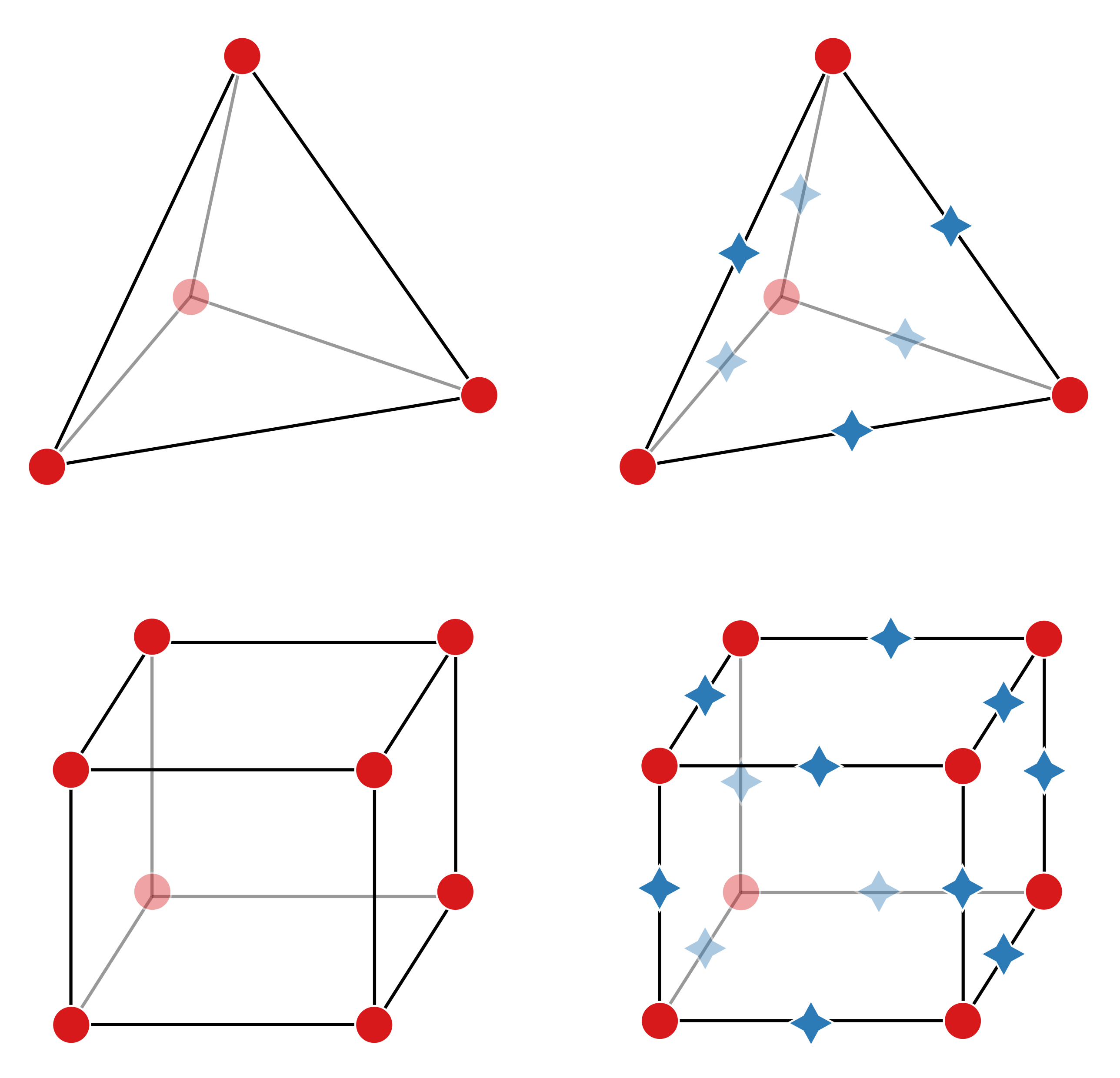
A critical aspect when facilitating close collaboration between architects and engineers is the consideration of model types. The primary purpose of an architectural model is to represent space. On the other side, a structural engineer aims to analyse the strength and stability of the under-laying structure. In an architectural model, all elements such as beams, columns, walls, and roofs generally have a three-dimensional boundary. It is not straightforward to convert these physical elements into elements compatible with an analytical model for finite element analysis. Depending on the problem, different element types may represent the physical situation. Real-world objects are broken down into smaller parts for the analysis, a process known as discretisation. The beam in Figure 3 use used as an example; the architectural beam has a width, depth, and length. Depending on the information sought and expected behaviour, the engineer may use a one-dimensional element such as a beam and bar element consisting of two end nodes connecting a straight line; each end node has degrees of freedom relevant to the problem. In other cases, a two-dimensional model may be more apt. Here the engineer discretises the beam into shell or plate elements. Apart from the type of element selected, the number of elements used will affect the accuracy of the solution. Finally, solid three-dimensional elements can be used as well. Here, all three dimensions represent the physical beam by “populating” it with discrete elements.

In most engineering problems related to architecture, one- and two-dimensional elements are sufficiently accurate and computationally effective. In Grasshopper 3D, there are also plugins for FEA internally or connecting to external FEA software such as Karamba3D, Sofistik^® and FEM-Design^®, respectively. These plugins take line- and surface geometries together with information about cross-sections and material as input for creating structural elements for the analytical model. However, in cases such as the one in this paper where small physical elements, the gridshell nodes, are subjected to sizeable forces, the assumptions necessary for the one- and two-dimensional elements to be valid are no longer applicable. For example, the premise of small deflection and plane sections remaining plane after deformation might not apply in a gridshell node. For these cases, a FEA using solid elements is necessary to evaluate the geometry accurately.

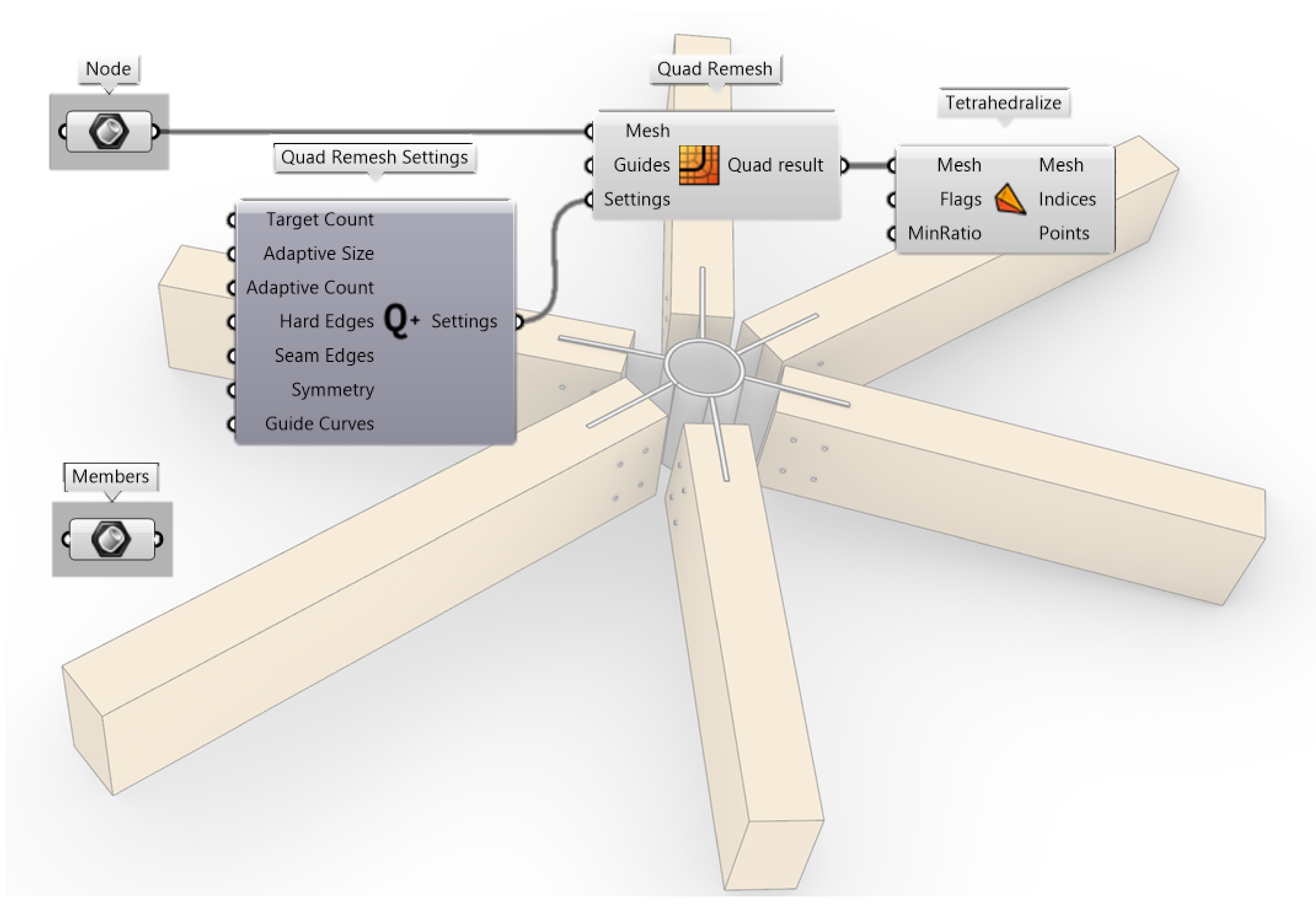
This raises the question of how to discretise a volumetric architectural element into small solid finite elements while working in the same software as the architect to maintain close collaboration. Most computer-aided design (CAD) software can easily discretise curves into a series of straight elements or a surface into a mesh of triangular or quad faces. Dividing a volumetric element into a solid mesh element is significantly more complicated. Normally, one would export the object and use different specialised software. As seen for Printshell discussed in Section 2.1, this is a timely procedure which impedes the creativity necessary in a conceptual design phase. Luckily, one of Grasshopper 3D’s greatest strengths is the possibility for third-party developers to create their own plugins within the program. The website food4Rhino.com [15] is a marketplace where these are distributed among users, often free of charge for non-commercial purposes. Here, the plugin Tetrino can be found [16]. 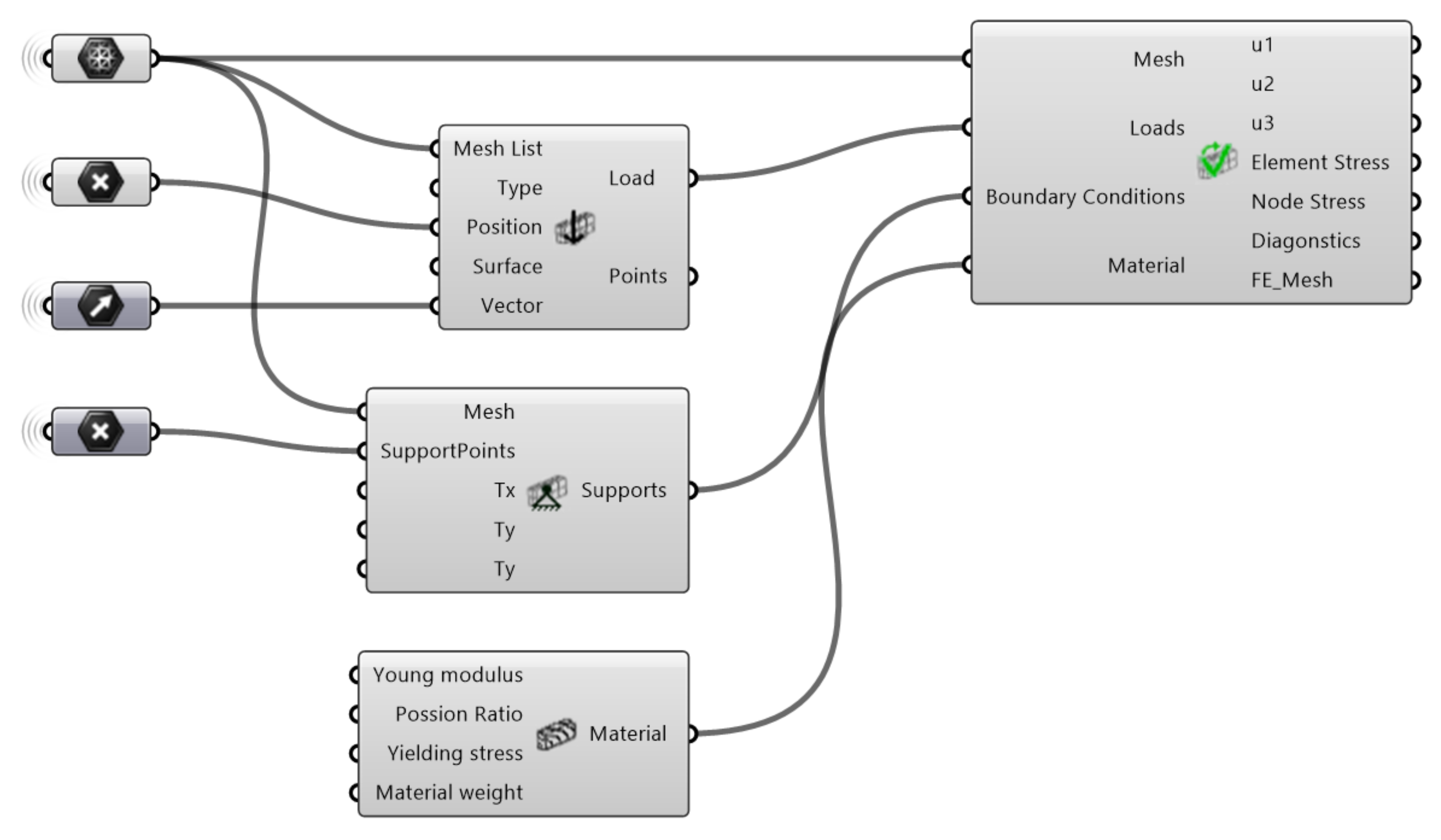This is a plugin working as a wrapper for the TetGen algorithm [17] that allows for the meshing of solid elements directly in Grasshopper 3D. Thus, a change in the architectural model can be automatically updated within Grasshopper 3D for the analytical model of the engineer. Despite the necessary geometric information and different possibilities for generating meshes for an FEA, there exists, to the authors’ knowledge, no tool that performs a complete FEA using solid elements within Grasshopper 3D today. Consequently, this paper presents the work to implement such a tool.

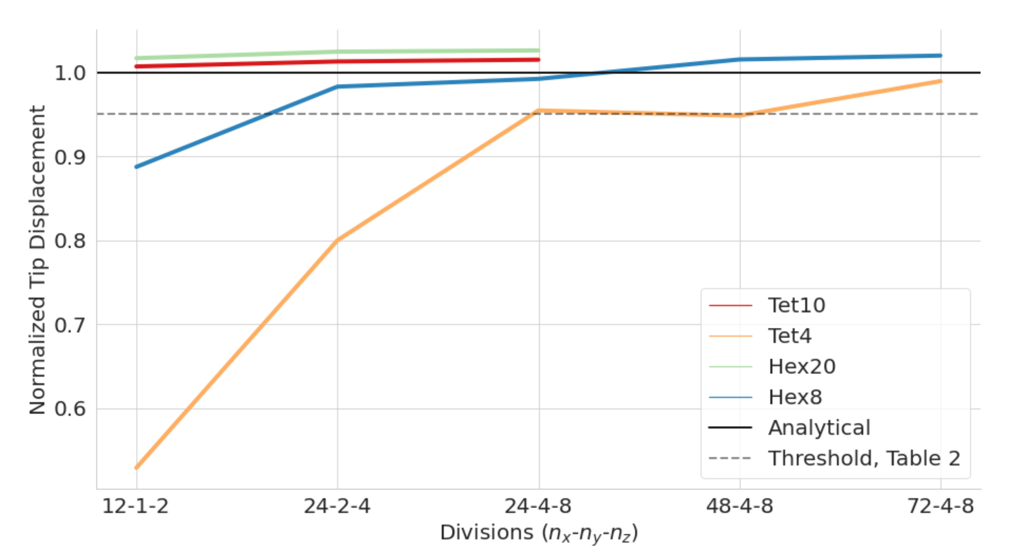
In order to test the efficiency and functionality of the plugin, a series of gridshell node geometries have been examined with the tool. A more thorough description of the methodology for developing gridshell nodes will be presented in another article by the authors. The selected nodes and the results from the case studies are presented in Section 4. The current version of this tool only supports linear analysis using isotropic material such as metal. Implementation of orthotropic material, nonlinearities and contacts are expected to be included in further versions. Due to these limitations, the case studies in this paper only consider the metal part of the nodes without any interaction between fasteners and timber beams.

3. The Solid FEA Plugin

A developed tool for FEA with solid elements is presented in this section as a way to answer the challenges raised in the previous section. The first subsection describes the third-party libraries necessary to handle the matrix operations before the architecture of the developed tool is described. Finally, a guide to using the tool is given together with a practical example in order to familiarise the reader with the concept.

3.1. .Net Libraries

As the finite element solver is dependent on multiple matrix operations, a fast and stable matrix library for .NET is necessary. The stiffness matrix in a structural problem mostly has zero-value entries; such a matrix is defined as a sparse matrix. Consequently, the plugin uses CSparse [18], a library optimised for operations on sparse matrices, as the matrix library. Additionally, the matrix library MathNet [19] is used for minor matrix operations and data storage throughout the library.

3.2. The Class Structure

In addition to Rhinoceros’s native geometry, some extensions are necessary to perform an FEA. Rhinoceros’s existing geometry classes, such as Point3d and Mesh, are used as attributes also for the finite element classes to keep everything as simple as possible. A simplified illustration of the pertinent classes is given in Figure 4. The Element class of the FEM library stores the equivalent Rhino Mesh instance as an attribute. In addition, some information about the local node’s place in the global mesh is necessary; this is the Connectivity field. Its Nodes and Type are also essential information that native Rhinoceros classes cannot provide. The Node-class is comparable to a Point3d, only with additional information regarding whether or not the nodes should be constrained from displacement during the analysis.

The FEMMesh-class stores all the individual elements and nodes of the structure to analyse. Moreover, it needs information about the object’s material. The Material class provides this information. At the moment, only isotropic material is implemented. The FEMesh also stores the results of the FEA. Stresses and displacements in both nodes and elements are stored as lists.

Available Element Types

There are currently four different element types implemented in the solver: First order and second order tetrahedron, Tet4 and Tet10, and first order and second order hexahedron, Hex8 and Hex20. As illustrated in Figure 5, the second order element has an extra node on the midpoint of all element edges in addition to the corner nodes that are shared with the first order element. By adding a middle node on the edges, the shape functions representing the displacement along the element are now nonlinear compared to the linear functions of the first order elements. Second order elements benefit from significantly increasing the accuracy of the analysis while using fewer elements in the mesh. Unfortunately, this comes with the cost of a more computationally expensive analysis, as demonstrated in Section 3.4.

3.3. A Summary of the Finite Element Procedure

The following subsection briefly describes the procedure of the FEA as the basic theory is outside the scope of this paper. The implementation is based on the book The Finite Element Method: its basis and fundamentals by Zienkiewicz et al. For a more elaborate description, refer to this [20].

Numerical integration is used to calculate each element’s local stiffness matrix. Here the element’s Cartesian coordinates are mapped to a dimensionless space where a Gauss quadrature is used for the integration over the volume. A part of the integration process is establishing the Jacobian matrix for each element. This matrix gives information relating to the element’s transformation going from Cartesian to dimensionless coordinates. As the accuracy of the analysis is dependent on relatively even mesh elements, the Jacobian (the determinant of the matrix) gives valuable information about this transformation. Skewed and heavily rotated elements have a negative impact on the accuracy of the analysis. Thus, elements where the Jacobian indicates this are logged as information for the user to keep in mind when interpreting the output. When each element is calculated, the matrix entries are added to the correct position in the global matrix according to the element’s connectivity.

With all the necessary data to establish the global stiffness matrix $\mathit{K}$ and the load vector $\mathit{R}$, the unknown displacement vector, $\mathit{v}$, is solved through the equation $\mathit{Kv}=\mathit{R}$. This is the most computationally expensive part of the algorithm due to the need for inverting the global stiffness matrix. As mentioned above, the CSparse library is used to solve this equation. The global stiffness matrix is converted to compressed column storage to create a lower-upper (LU) decomposition before solving for the array of displacement values in each node. With the nodal displacement in all the nodes, the next step is to calculate nodal strain and stresses. For this, the strains are obtained using each element’s B-matrix evaluated in all Gauss points. These strains are then extrapolated back to the element nodes by multiplying the strains in the Gauss points with the shape function values in each element node. Now, all the elements’ nodal strains in each element are obtained. The final operation is then to assign the stresses to each FE Element and assemble all the information in the FEMesh class, which is the output of the analysis.

From here, all the information required to evaluate the analysed geometry’s performance is available. The evaluation can either be done visually, through a preview component where the displacements and various stresses are illustrated by colours, or numerically by actual values. A combination of both is also an option. Even for users without a technical background, the coloured mesh displaying the utilisation in percentage is particularly useful. With such visualisation, it is possible to intuitively inspect the flow of forces and get an initial expectation of the geometry’s behaviour.

3.4. Introducing the Components: Analysing a Cantilevering Beam

This subsection presents the plugin’s components through a practical example. The cantilevering beam in Figure 6 is analysed, and the performance of the available element types is evaluated and compared to the analytical solution as a benchmark. The beam has a length, L of 1200 mm, and a point load, P, of 150 kN is applied at the end. Further information about the cross section’s widh, w, and height, h, together with the Young’s modulus, E, yield stress, $f_{yd}$, and Poisson’s ratio, $\nu$, are provided in

Table 1. Input data for the cantilever beam.

L [mm]	w [mm]	h [mm]	E [GPa]	${\mathit{f}}_{\mathit{yd}}$ [MPa]	$\mathit{\nu }$	P [kN]
1200	100	200	200	355	0.3	150

.

3.4.1. Establishing the Model

Figure 7 demonstrates the components necessary for establishing the FEA using the presented plugin. A brief description of each step follows.

For the analysis to run, the FEMSolver component requires a list of Rhino meshes. These can be either tetrahedrons or hexahedrons analogous to the first order finite elements Tet4 and Hex8 in Figure 5. In this example, the meshes are generated by a C# script to have complete control of division number and element types, but for more arbitrary and complex geometry, a meshing algorithm is recommended. In this analysis, the number of divisions in the x-, y-, and z-direction is user input, and hexahedral elements are created accordingly. Each hexahedral is divided into six tetrahedrons for tetrahedral elements, i.e., for the same division number, the tetrahedral mesh will have six times as many elements. In cases where the user wants second order elements for the analysis, the mesh input in Figure 7 is passed through a component which adds a node to the middle of all mesh edges seen in Figure 8. This modified mesh is then the mesh input in all the FEA components. Apart from that, everything remains the same.

Next, the mesh points where boundary conditions apply have to be specified. The Support component takes the mesh list as input together with the point to restrain from translation in directions specified by the user. By default, all three translations are restrained, but this can be modified by changing the Boolean values of Tx, Ty, and Tz in the component. The component’s output is a list of 0’s and 1’s representing the constraint from translation in all nodal directions. 0 indicates a free node, whereas 1 indicates a restraint.

Similarly to the boundary conditions, the location of the applied loads needs to be specified. Here, both point and surface loads can be applied. The necessary inputs are the mesh list, the type of load (0 for surface- and 1 for point load), the surface or points to assign the loads to, and the vector specifying the direction of the load. The output is a list corresponding to the global load vector, and a list of points on the mesh where a load is acting for the user to verify the results.

Finally, the object’s material needs to be specified using the Material component. By default, the properties of S355 steel are set as input values, but the user may change these if necessary. With isotropic material, the only necessary inputs are the Young’s modulus, Poisson Ratio, Yield stress, and material weight.

With all necessary parameters defined, the analysis is done by connecting all the above inputs into the FEMSolver. After running the analysis, the results are stored in the FEMesh class, which is also an output of the solver. This can be used later for the visualisation of the results. In addition, the solver outputs lists of nodal displacements in u-, v-, and w- directions, as well as lists of nodal en element stresses. The final output is a list of strings giving information about the analysis.

3.4.2. Results from the Analysis

Having described how each component works to establish an analysis, the section ends by looking at the results using different element types. As a reference, an analytical solution of the beam’s tip deflection, ${\delta }_{max}$, and maximum bending stresses, ${\sigma }_{xx.max}$, are used. The formulas for calculating these values are given as:

$${\delta }_{max}=\frac{P{L}^3}{3EI},{\sigma }_{xx.max}=\frac{6PL}{w{h}^2}$$

(1)

where $I=\frac{1}{12}w{h}^3$ is the second moment of inertia for a rectangular cross section. Inserting the relevant values into (1) results in a maximum deflection of $6.48$ mm and maximum stress of 270 MPa. Below,

Table 2. Overview of the number of elements necessary for different element types to achieve an accuracy of at least 95% compared to the analytical solution of 6.48 mm. The run time for each analysis is included in the rightmost column. Note that $n_{els}$ for Tet4- and 10 are obtained by multiplying the product of Divisions with 6 as each hexahedron is divided into six tetrahedrons.

Element Type	Divisions	${\mathit{n}}_{\mathit{els}}$	${\mathit{\delta }}_{\mathit{max}}$	${\mathit{\sigma }}_{\mathit{xx}}$	Run Time [ms]
Tet4	24-4-8	4608	0.95	0.89	5007
Tet10	12-1-2	144	1.01	1.04	127
Hex8	24-2-4	192	0.98	0.98	171
Hex20	12-1-2	24	0.98	1.04	233

presents the the elements’ normalised displacements and bending stresses, with respect to the analytical values, for the minimum number of elements, $n_{els}$, where the accuracy is at least 95% of the analytical solution.

As expected, the linear tetrahedron element, Tet4, has the lowest accuracy and longest computational time. The extremely high computational time is caused by the number of elements being more than ten times greater than both the Tet10 and Hex8 elements. For a bending problem with linear stress distribution over the beam’s height, there is a need for many linear elements as they only have the ability to represent constant stress within each element. It is worth noting that for a uniformly distributed load along the top of the beam, the Tet4 element is expected to perform even worse with the bending moment along the beam length varying with a quadratic instead of linear shape. Thus, an even higher number of elements is necessary to approximate the exact stress distributions within the beam. Using Tet10 elements, both the efficiency and accuracy drastically increase. Here, only 144 elements are necessary to achieve satisfying results, with a run time of 127 milliseconds. For the hexahedral elements, the same trend is visible. A finer mesh with more elements is necessary to achieve accurate results for the linear Hex8 element. The Hex20 only need 24 elements, but comes at the cost of more computational time.

Figure 9 shows the convergence of displacement of the different element types toward the analytical solution. This plot further emphasises the need for more linear elements shown in Table 2. Both Tet10 and Hex20 can reproduce accurate solutions for a coarse mesh, whereas the linear elements have slower convergence towards the exact solution. As this plot shows, the user should pay extra attention when working with linear tetrahedral elements in problems where bending moments are present, such as this cantilevering beam.

To summarise the chapter, it is relatively straightforward to establish an analysis from the existing Grasshopper geometries. A list of tetrahedral or hexahedral mesh instances is created, and the nodes or surfaces where the loads and boundary conditions are applied are selected together with constraints and load vectors. Finally, an isotropic material is given together with the other input to the solver component. The output is an instance of the finite element mesh with results and lists of displacements and stresses in both nodes and elements. Using nonlinear elements such as Tet10 and Hex20 yields better accuracy but comes at the cost of computation time. Depending on the problem at hand, the user should select a mesh accordingly.

4. Analysing Gridshell Nodes with Solid Elements

This section presents the application of the proposed tool on gridshell nodes. Four nodes with differing concepts for manufacturing procedure and load transfer have been selected. As discussed in Section 2.2, the assumption of rigid connections between nodes and elements is not a conservative one. Moreover, with the architect exploring novel node designs, the node’s behaviour is generally interesting. In such cases, a detailed analysis of this part is necessary. All the nodes are proposed for a timber gridshell with metal nodes, but in these case studies, only the metal part has been examined due to limitations with the tool as mentioned in Section 2.3. The following subsection presents a typical workflow using selected nodes.

4.1. Node Proposals for Evaluation

The Glued Finger node, shown in Figure 10a, has pre-assembled grippers glued to the timber. The grippers incorporate a wedge used for mechanical attachment to the node. The node-angles are handled by the twist and tilt of the node, whereas the grippers are all equal. The node itself is a star-like object with an even thickness along the flanges. The Mero ZK, shown in Figure 10b, is a hollow cup that handles the node angles. It has flat machined sides that flush with the member end faces and connects to the members with bolts inserted from the inside of the cup that attaches to glued in double-threaded rods in the members. The Starnode, shown in Figure 10c, is a monolithic core that connects to the members using threaded rods. The node handles the node-angles and attaches to the members to the end faces. The node is hollow to reduce weight and produced using casting. The Polo-1, shown in Figure 10d, is an adaptation of a very common gridshell node. It is produced from a hollow tube with welded vertical splices. The splices have holes for attaching to the timber with bolts.

4.2. Global to Local Gridshell Analysis

The node geometries of interest in Figure 10 are developed as separate Grasshopper scripts. The first part of the analysis involves an initial analysis of the global gridshell model using beam elements with the Grasshopper^® plugin Karamba3D. From this, a single node and the belonging elements of interest are extracted together with the normal- (N) and shear (V) forces, and moments (M) coming into the node from each element. The forces for the relevant members are presented in

Table 3. The forces at each of the members that are attached to the selected node.

Bar ID	N (Fx) kN	V (Fv) kN	M (My) kNm
2328	68.6	3.04	−15.79
2410	−16.12	−0.35	−0.99
2407	−5.52	−0.6	−2.3
2340	62.99	−2.19	−14.49
2327	−14.27	0.7	−3.05
2326	−7.37	0.08	−0.54

, together with the global ID of each bar. Given the architectural model of the same part of the gridshell, the remainder of this section illustrates how the presented tool can link the architectural model to an FEA with solid elements directly in Grasshopper.

4.3. Preparing the Node Geometries

Figure 11 illustrates the architectural model of geometries provided by the architect, one brep (boundary representation) representing the node and six breps for the members, together with the meshing of the node. Here, the Tetrino plugin discussed in Section 2.3 is used to create a mesh of tetrahedrons from the brep after an initial surface meshing of the brep with the Quad Remesh component.

The next step is to identify the mesh’s nodes for which we want to apply loads and boundary conditions. There are several ways of doing this in Rhino; for this example, all vertices of the tetra mesh are projected onto each member, and the vertices that have translated below a specified limit distance are selected as the load or boundary nodes. Subsequently, the element forces must be distributed as nodal forces onto the appropriate nodes and in the correct direction. Again, the existing information in the architectural file is utilised. This time, using the plane of the breps’ surface that faces the node’s plane. U- and v-vectors of this planar face correspond to the direction vectors of the normal and shear forces. Finally, the moments are simplified as pairs of opposite forces along the members’ x-axis. With this, all the necessary input data corresponding to Figure 7 is available, and the user can evaluate the performance of the proposed nodes.

4.4. The Meshing and Analysis of the Nodes

With the script presented above, the outcome is the meshed nodes presented in Figure 12. Although the connections between the beams and nodes are different for the various types, the algorithm automatically identifies the contact areas and applies both loads and boundary conditions. The red points on each mesh illustrate points where a load or boundary is added.

Figure 13 shows the nodes after analysis with a colour map of the magnitude of displacement in each meshed node. This map can be used to identify which parts of a connector that is deflecting the most for a given load case. In addition to the colouring, the displacements can be simulated by scaling the translation of the mesh in the Rhinoceros viewport using a slider. When combined, this gives the user a solid understanding of how the node behaves under the present loading condition. Another, more advanced possibility, when working on a linear analysis, is to extract the deflection of specific nodes when subjected to a pre-defined load to estimate the rotational- and translational stiffness of the elements as well. This can then be used to update the rigidity of the global model in order to understand the gridshells’ behaviour better.

Finally, the stresses and utilisation in the node can be visualised similarly to the displacements, as shown in Figure 14. Here, the ${\sigma }_{xx}$ stresses are illustrated. Moreover, the user can select utilisation based on Von Mises, ${\sigma }_{yy}$, ${\sigma }_{zz}$, ${\sigma }_{xy}$, ${\sigma }_{xz}$, and ${\sigma }_{yz}$. As for the displacements, the numerical values can be extracted as lists with indices corresponding to the ID of each node and element. With the given load case from Table 1, two of the incoming members have significantly greater forces than the remaining four. This can be seen in the stress plots as well, with the colour intensity being greatest in two of the six arms. As the colour map of the stresses illustrates, the different types of nodes have high stress concentrations in different areas of the node as well. For the Glued Finger node in Figure 14a, the short distance between the timber part and the node’s centre gives relatively uniform compression stresses close to the centre compared to Starnode in Figure 14c, which has more significant stress closer to the beams. In the Polo-1 node, Figure 14d, the arms of the nodes are “pushing” and “pulling” on the inner ring and deforming this. For the Mero ZK, Figure 10b, the local stresses where the bolts connect node and members were modelled. This results in significantly higher stresses in this area compared to the rest of the node, as shown in Figure 14b—indicating that the bolt dimension and metal thickness in this node are critical parts of the connection.

Although not a complete design verification, this section has demonstrated how the architectural and analytical model can be linked using the presented tool inside Grasshopper 3D. The opportunity to get performance feedback during design exploration is believed to enhance the final result as well as the collaboration between architect and engineer.

5. Conclusions

This paper presented a novel tool for volumetric FEA implemented as a plugin for Grasshopper. The challenges of working with architectural and analytical models in the same environment were discussed. Especially for problems where existing FEA software using one- and two-dimensional finite elements are insufficient. The nodes in a gridshell are an example; in a global structural model, these are normally assumed as rigid joints between elements, resulting in a “too stiff” global model. Subsequently, the proposed FEA tool using solid finite elements was presented and verified on a cantilevering beam example. After that, a case study demonstrated how the presented tool could be used to evaluate several proposals for gridshell nodes directly in Grasshopper 3D, provided only the geometry model and forces from a global structural analysis.

Although the tool has great potential, the development of the tool is at an early stage. Consequently, there are bugs in the analysis, and multiple functions are missing that would further strengthen the tool. For the finite element framework, the inclusion of more element types, orthotropic material, selective reduced integration of the elements, hourglass control, and contact problems are common in most commercial finite element software and would also significantly improve the proposed tool’s efficiency. Another limitation is the number of elements in the meshed geometry that the solver can compute for a solution in Grasshopper 3D. When exceeding approximately 18,000 elements, the component can no longer establish the global stiffness matrix of the system. To remedy this, future work and updates of the tool includes both an optimised architecture of the developed components and parallel threading which can allow denser mesh and larger objects in the analysis. Moreover, future work should utilise the tool in physical prototyping of gridshell nodes. Finally, the aim is to publish the tool and make it publicly available on food4Rhino. Despite its limitations, the tool provided quick analyses on gridshell nodes where the geometry was defined within Grasshopper 3D. We are certain that many other applications will be found when the tool is made publicly available.

References

1. Rutten, D.; McNeel, R. Grasshopper3D; Robert McNeel & Associates: Seattle, WA, USA, 2007. [Google Scholar]
2. Preisinger, C. Linking structure and parametric geometry. Archit. Des. 2013, 83, 110–113. [Google Scholar] [CrossRef]
3. Kohnke, P. Ansys. In Finite Element Systems; Springer: Berlin/Heidelberg, Germany, 1982; pp. 19–25. [Google Scholar]
4. Lara-Bocanegra, A.J.; Majano-Majano, A.; Ortiz, J.; Guaita, M. Structural Analysis and Form-Finding of Triaxial Elastic Timber Gridshells Considering Interlayer Slips: Numerical Modelling and Full-Scale Test. Appl. Sci. 2022, 12, 5335. [Google Scholar] [CrossRef]
5. Lopez, A.; Puente, I.; Aizpurua, H. Experimental and analytical studies on the rotational stiffness of joints for single-layer structures. Eng. Struct. 2011, 33, 731–737. [Google Scholar] [CrossRef]
6. Fan, F.; Ma, H.; Cao, Z.; Shen, S. A new classification system for the joints used in lattice shells. Thin-Walled Struct. 2011, 49, 1544–1553. [Google Scholar] [CrossRef]
7. Seifi, H.; Rezaee Javan, A.; Xu, S.; Zhao, Y.; Xie, Y.M. Design optimization and additive manufacturing of nodes in gridshell structures. Eng. Struct. 2018, 160, 161–170. [Google Scholar] [CrossRef]
8. El-Sheikh, A. Development of a new space truss system. J. Constr. Steel Res. 1996, 37, 205–227. [Google Scholar] [CrossRef]
9. Cuvilliers, P.; Douthe, C.; du Peloux, L.; Roy, R.L. Hybrid structural skin: Prototype of a GFRP elastic gridshell braced by a fiber-reinforced concrete envelope. J. Int. Assoc. Shell Spat. Struct. 2017, 58, 65–78. [Google Scholar] [CrossRef]
10. Bo, P.; Pottmann, H.; Kilian, M.; Wang, W.; Wallner, J. Circular Arc Structures. ACM Trans. Graph. 2011, 30, 101. [Google Scholar] [CrossRef]
11. Dyvik, S.H.; Manum, B.; Rønnquist, A. Gridshells in Recent Research—A Systematic Mapping Study. Appl. Sci. 2021, 11, 11731. [Google Scholar] [CrossRef]
12. Castriotto, C.; Tavares, F.; Celani, G.; Larsen, O.P.; Browne, X. Clamp links: A novel type of reciprocal frame connection. Int. J. Archit. Comput. 2021, 14780771211054169. [Google Scholar] [CrossRef]
13. Harris, R.; Gusinde, B.; Roynon, J. Design and construction of the pods sports academy, Scunthorpe, England. In Proceedings of the World Conference of Timber Engineering 2012, Auckland, New Zealand, 15–19 July 2012. [Google Scholar]
14. Stephan, S.; Sánchez-Alvarez, J.; Knebel, K. Reticulated structures on free-form surfaces. Stahlbau 2004, 73, 562–572. [Google Scholar] [CrossRef]
15. Food4Rhino. Available online: https://www.food4rhino.com/en (accessed on 20 May 2022).
16. Svilans, T. Tetrino. 2022. Available online: https://github.com/tsvilans/tetrino (accessed on 20 May 2022).
17. Hang, S. TetGen, a Delaunay-based quality tetrahedral mesh generator. ACM Trans. Math. Softw. 2015, 41, 11. [Google Scholar]
18. Davies, T. CSparse. 2022. Available online: https://github.com/DrTimothyAldenDavis/SuiteSparse/tree/master/CSparse (accessed on 20 May 2022).
19. Ruegg, C. MathNet.Numerics. 2022. Available online: https://github.com/mathnet/mathnet-numerics (accessed on 20 May 2022).
20. Zienkiewicz, O.C.; Taylor, R.L.; Zhu, J.Z. The Finite Element Method: Its Basis and Fundamentals; Elsevier: Amsterdam, The Netherlands, 2005. [Google Scholar]
Figure 1. The node at the Printshell project and the ANSYS analysis at the project.
Applsci 12 06037 g001
Figure 2. Illustration of the node angles U, V and W.
Applsci 12 06037 g002
Figure 3. The architectural model of a beam represented as 1D, 2D, and 3D analytical elements.
Applsci 12 06037 g003
Figure 4. Class diagram showing the classes used to generate the FEA.
Applsci 12 06037 g004
Figure 5. Currently available element types in the plugin. (Top): First and second order tetrahedron. (Bottom): First and second order hexahedron.
Applsci 12 06037 g005
Figure 6. Illustration of benchmark problem. A cantilevering beam with a cross-section of 100 mm × 200 mm. The theoretical solution, using beam theory, is used as a reference for the analysis.
Applsci 12 06037 g006
Figure 7. Necessary components for establishing an FEA. The left column represents containers for native Rhino geometry, the middle column the components for creating loads and supports, while the right component assembles and analyses the mode.
Applsci 12 06037 g007
Figure 8. The component that adds a middle node on all mesh edges for quadratic finite elements.
Applsci 12 06037 g008
Figure 9. Convergence plot of the available element types for the normalised displacements of the cantilever example. The analytical solution is plottet as a straight line, while the threshold value for Table 2 is dashed.
Applsci 12 06037 g009
Figure 10. The four node geometries that will be evaluated using this section’s proposed workflow. (a) Illustration of the Glued Finger Node. (b) Illustration of the Mero ZK. (c) Illustration of the Starnode. (d) Illustration of the Polo-1.
Applsci 12 06037 g010
Figure 11. The geometry provided by the architect and the meshing of the node for the analysis.
Applsci 12 06037 g011
Figure 12. Meshed versions of the four node proposals. Red dots indicate positions where loads or boundary conditions are applied. (a) Meshed Glued Finger Node. (b) Meshed Mero ZK. (c) Meshed Starnode. (d) Meshed Polo-1.
Applsci 12 06037 g012
Figure 13. Displacement plots of the nodes. The hue of the colour illustrates the magnitude of displacements. (a) Displacements in the Glued Finger Node. (b) Displacements in the Mero ZK. (c) Displacements in the Starnode. (d) Displacements in the Polo-1.
Applsci 12 06037 g013
Figure 14. Stress plots for the nodes. The intensity of colours matches the intensity of stresses. (a) Stress concentrations in the GF Node. (b) Stress concentrations in the Mero ZK. (c) Stress concentrations in the Starnode. (d) Stress concentrations in Polo-1.
Applsci 12 06037 g014