Modified A-Star (A*) Approach to Plan the Motion of a Quadrotor UAV in Three-Dimensional Obstacle-Cluttered Environment

Abstract

Motion-planning algorithms play a vital role in attaining various levels of autonomy for any ground or flying agent. Three-dimensional (3D) motion-planning is interesting, but rather complex, especially for flying agents such as autonomous unmanned aerial vehicles (UAVs), due to the increased dimensionality of space and consideration of dynamical constraints for a feasible trajectory. Usually, in 3D path search problems, it is hard to avoid extra expanded nodes due to increased dimensionality with various available search options. Therefore, this paper discusses and implements a modified heuristic-based A* formalism that uses a truncation mechanism in order to eradicate the mentioned problem. In this formalism, the complete motion planning is divided into shortest path search problem and smooth trajectory generation. The shortest path search problem is subdivided into an initial naïve guess of the path and the truncation of the extra nodes. To find a naïve shortest path, a conventional two-dimensional (2D) A* algorithm is augmented for 3D space with six-sided search. This approach led to the inclusion of extra expanded nodes and, therefore, it is not the shortest one. Hence, a truncation algorithm is developed to further process this path in order to truncate the extra expanded nodes and then to shorten the path length. This new approach significantly reduces the path length and renders only those nodes that are obstacle-free. The latter is ensured using a collision detection algorithm during the truncation process. Subsequently, the nodes of this shortened path are used to generate a dynamically feasible and optimal trajectory for the quadrotor UAV. Optimal trajectory generation requires that the plant dynamics must be differentially flat. Therefore, the corresponding proof is presented to ensure generation of the optimal trajectory. This optimal trajectory minimizes the control effort and ensures longer endurance. Moreover, quadrotor model and controllers are derived as preliminaries, which are subsequently used to track the desired trajectory generated by the trajectory planner. Finally, results of numerical simulations which ultimately validate the theoretical developments are presented.

1. Introduction

Scientific developments in the field of micro unmanned aerial vehicles (UAVs) have made it possible to accomplish numerous daily life challenges for which human deployment may possess a probable life risk, e.g., surveillance of damaged nuclear reactors, reconnaissance missions in hostile environments, surveillance of damaged buildings in earthquake-affected areas, etc. [1,2,3,4,5,6]. In recent warfare zones, UAVs can act as smart mobile weapons, which can search for a specific target by recognizing the facial features or other prescribed characteristics of the target. Due to its vertical takeoff and landing (VTOL), perching ability, and quasi-stationary flight attributes, the quadrotor UAV has garnered much attention from the research community as compared to other UAVs [7,8]. For any robot, the central motive for novelties and research expansions is to bring about ultimate autonomy and intelligence. Therefore, during the past several years, researchers have contributed significantly in the fields of design, intelligent control, trajectory generation, and motion-planning to enhance the autonomy level of micro quadrotor UAVs [9,10,11,12,13,14,15].

Motion-planning has widely been investigated for robots operating in various kinds of environments, and several methods exist to search for a path in obstacle-cluttered environments [16,17,18,19,20]. Dijkstra is an earlier and simpler version developed to find the shortest path on a map. Later, it was improved, and the subsequently developed algorithm is known as a greedy best-first search algorithm, which works in a similar fashion as does Dijkstra. However, the latter incorporates guided search through heuristics, which helps in estimating how far the goal is from any current vertex. The Dijkstra algorithm works in all directions simultaneously and is therefore computationally costly for three-dimensional motion-planning. However, it is guaranteed to find the shortest path. Contrarily, greedy best-first search algorithm works in a guided direction and runs quickly. However, the path found is not guaranteed to be the shortest. Therefore, it only focuses on the cost to reach the goal point and ignores the cost of the path, which is the major drawback of this algorithm. The promising solution is the combination of both aforementioned algorithms, and the consequence is known as A* algorithm, i.e., A-star. A* is the most popular algorithm in pathfinding problems, and it has been used extensively in numerous ground robotic path search applications [17,18,19,20,21,22]. Extension of A* to 3D space poses the issue of exploration of extra nodes that result in a suboptimal path. Such suboptimal paths will render a trajectory that increases the control effort of the UAV and obviously reduces the flight endurance.

Autonomous navigation of a micro quadrotor UAV through obstacles cluttered in a three-dimensional space requires fast search algorithms featuring the ability of map-reading in order to generate a shortest collision-free path between initial and final positions. The generated shortest path must be dynamically feasible, smooth, and optimal [23,24,25,26,27,28]. A typical motion-planning problem involves two entities; one is the determination of the shortest collision-free path between start and final goal positions using the search algorithm, and the other is the generation of a dynamically feasible trajectory by taking into account the found shortest path [29,30,31]. Most of the commonly used search algorithms for solving autonomous robot navigation problems are graph-theory-based, and the generated shortest path always contains infinite curvatures [32,33,34,35]. This ultimately implies certain unwanted limitations on quadrotor mission profile, i.e., quadrotor dynamics cannot handle infinite curvatures and it must stop at these points. To eradicate this limitation in our work, the shortest path found by the search algorithm is handed over to a trajectory generation algorithm, which generates a dynamically feasible and optimal trajectory with finite and smooth curvatures. The vibration of the UAV frame [36,37] and the motion of a robot manipulator mounted on the UAV [38] might affect the system dynamics and motion planning, and this will be investigated in future works. In particular, a reactionless motion of the manipulator [39,40,41,42] will be beneficial because it will not significantly affect the system dynamics.

Most of the search algorithms present in the literature have only been investigated for ground robotic applications, and therefore, their implementation is limited only to two-dimensional cases. However, this paper augments a heuristic-based A* search algorithm from a two-dimensional scenario to three-dimensional space, and this work specifically involves a quadrotor UAV traversing the generated shortest path. The major contribution of this paper is the development of modified A* formalism in order to plan a motion for a quadrotor UAV in a 3D space. This includes the generation of a dynamically feasible trajectory to reduce the control effort as well. In 3D space, a conventional A* approach may expand extra nodes if its expansion is kept to six neighboring sides. Therefore, in many scenarios, the searched 3D path may not be the shortest one and can involve extra nodes. In this work, we have modified the conventional approach of an A* algorithm by developing a truncation algorithm which takes the path nodes computed using A* as input. The modified approach guarantees a collision free shortest possible path by truncating the extra nodes. These nodes of the determined shortest path are then used to generate a dynamically feasible trajectory using the differential flatness theorem. Various constraints have been considered in order to generate an optimal trajectory using the Euler–Lagrange formalism. This optimal trajectory reduces control effort and enhances the flight endurance of the UAV. Subsequently, the generated trajectory is followed autonomously by a micro quadrotor UAV in order to validate the developments of this work.

The rest of the paper is organized as follows: Section 2 presents a dynamical model of micro quadrotor UAV and controller structure which are subsequently used to traverse the generated trajectory. Section 3 explains the modified A* algorithm and trajectory generation. Section 4 illustrates the results of numerical simulations performed in MATLAB. Finally, Section 5 concludes the contribution and developments of this study.

2. Preliminaries

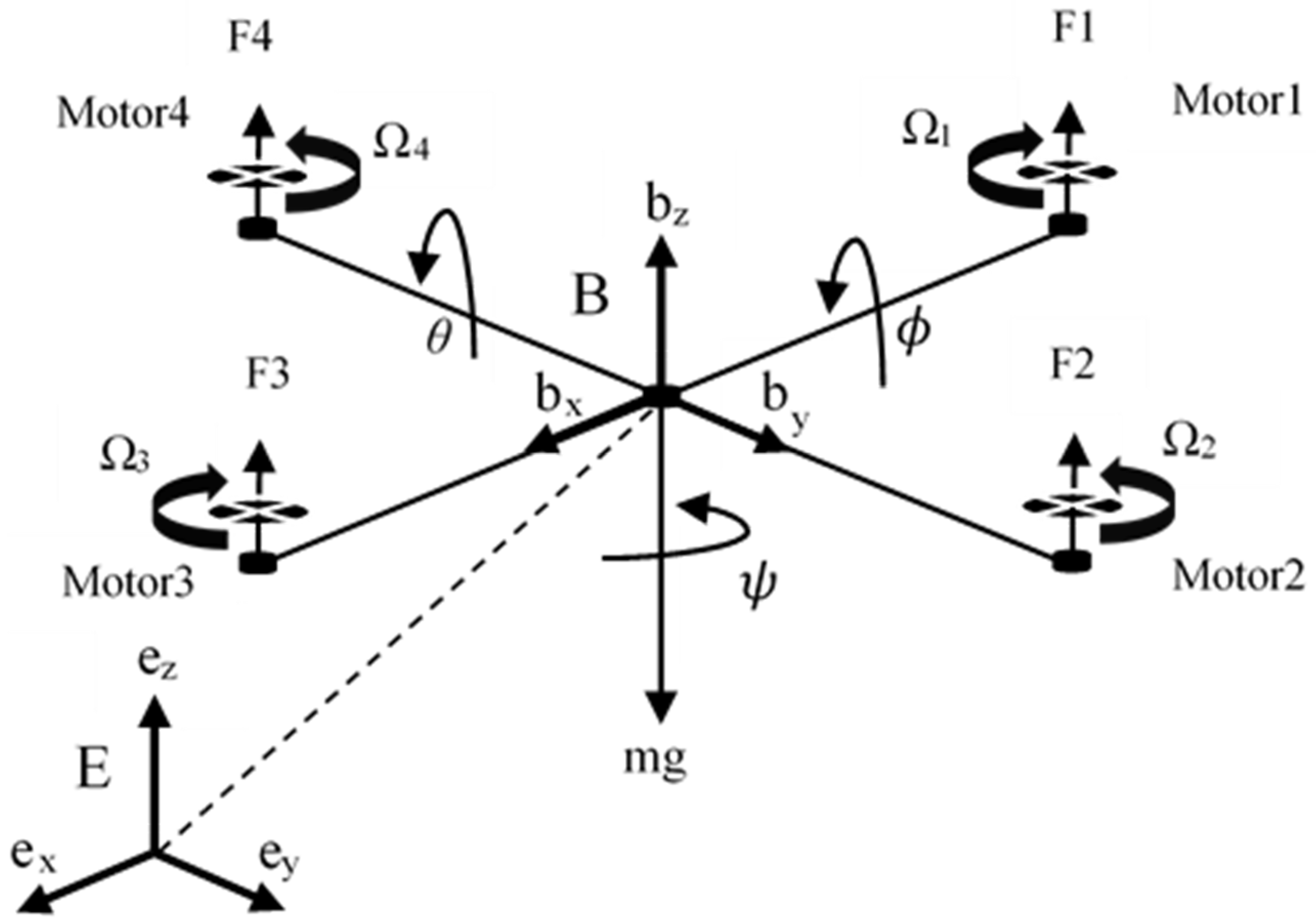
2.1. Modeling

A brief discussion on quadrotor modeling is presented in this section. The model is derived using Newton–Euler methodology, which has subsequently been used to derive a model-based flight controller. Referring to Figure 1, two reference frames are used to describe the motion of the aerial vehicle. The frame fixed to body is represented by $B=\left[\begin{array}{ccc}{b}_x& b_y& b_z\end{array}\right]$, while the frame attached to the earth is characterized by $E=\left[\begin{array}{ccc}{e}_x& e_y& e_z\end{array}\right]$. The earth-fixed frame is also known as inertial reference frame in most of the studies. The rotational motions across x, y and z-axes are called roll, pitch and yaw, respectively. These are symbolized by vector ${[\begin{array}{ccc}\varphi & \theta & \psi \end{array}]}^T$, and the corresponding body angular rates are represented by ${\omega }_B={[\begin{array}{ccc}p& q& r\end{array}]}^T$.

From Newton–Euler equations, the position ${\zeta }_O^E$ of the center of quadrotor body and velocity $V_O^E$ can be expressed as:

$$\raisebox{1ex}{$d{\zeta }_O^E$}\!\left/ \!\raisebox{-1ex}{$dt$}\right.=V_O^E$$

(1)

$$\raisebox{1ex}{$d{V}_O^E$}\!\left/ \!\raisebox{-1ex}{$dt$}\right.=-g{e}_z+R\frac{F_B}{m}{e}_z$$

(2)

$$\raisebox{1ex}{$dR$}\!\left/ \!\raisebox{-1ex}{$dt$}\right.=R S\left({\omega }_B\right)$$

(3)

where $g$ is gravity, $F_B$ is vertical thrust, $m$ is body mass, R is rotation matrix and $S\left({\omega }_B\right)$ is a skew symmetric matrix.

$$S\left({\omega }_B\right)=\left[\begin{array}{ccc}0& -r& q\\ r& 0& -p\\ -q& p& 0\end{array}\right]$$

(4)

In the inertial reference frame, the rate of change of angular momentum of the quadrotor body relative to its origin is equal to the total moment that results from all external forces that acts on the quadrotor body. This can be written as:

$$\raisebox{1ex}{$d^E{H}_O^E$}\!\left/ \!\raisebox{-1ex}{$dt$}\right.={\tau }_B$$

(5)

The ${\tau }_B$ is the net moment of the body produced by the external forces and torques about the origin O, while $H_O^E$ is the angular momentum in inertial reference frame E and is equal to $I_O{\omega }_B^E$. The term $I_O$ denotes an inertia tensor with O as its origin; ${\omega }_B^E$ is body angular rates in the inertial reference frame and is equal to $p{b}_x+q{b}_y+r{b}_z$.

Equation (5) can be written in the body reference frame as follows:

$$\raisebox{1ex}{$d^E{H}_O^E$}\!\left/ \!\raisebox{-1ex}{$dt$}\right.={\tau }_B$$

(6)

where $\raisebox{1ex}{$d^B{H}_O^B$}\!\left/ \!\raisebox{-1ex}{$dt$}\right.=I_x\dot{p}{b}_x+I_{y}q{b}_y+I_{z}r{b}_z$, ${\omega }_B\times H_O^B$ is the Coriolis effect and $\omega \times \lceil \begin{array}{c}0\\ 0\\ I_r{\mathsf{\Omega }}_r\end{array}\rceil$ is gyroscopic effect.

$$\lceil \begin{array}{ccc}{I}_x& 0& 0\\ 0& I_y& 0\\ 0& 0& I_z\end{array}\rceil \lceil \begin{array}{c}\dot{p}\\ \dot{q}\\ \dot{r}\end{array}\rceil +\lceil \begin{array}{ccc}0& -r& q\\ r& 0& -p\\ -q& p& 0\end{array}\rceil \lceil \begin{array}{ccc}{I}_x& 0& 0\\ 0& I_y& 0\\ 0& 0& I_z\end{array}\rceil \lceil \begin{array}{c}p\\ q\\ r\end{array}\rceil +\lceil \begin{array}{c}q{I}_r{\mathsf{\Omega }}_r-0\\ 0-p{I}_r{\mathsf{\Omega }}_r\\ 0\end{array}\rceil =\lceil \begin{array}{c}{\tau }_{B\varphi }\\ {\tau }_{B\theta }\\ {\tau }_{B\psi }\end{array}\rceil$$

(7)

As the name suggests, a quadrotor possesses four actuator entities called rotors, which produce two major dynamic terms. One is vertical thrust, or the lift force, and the other is the moment around the axis of rotation of the rotors. Lift force is central to performing any type of quadrotor maneuver, and its various combinations give the following four control terms:

$$\begin{array}{l}{F}_B=b\left({\mathsf{\Omega }}_1^2+{\mathsf{\Omega }}_2^2+{\mathsf{\Omega }}_3^2+{\mathsf{\Omega }}_4^2\right)\\ {\tau }_{B\varphi }=lb\left({\mathsf{\Omega }}_4^2-{\mathsf{\Omega }}_2^2\right)\\ {\tau }_{B\theta }=lb\left({\mathsf{\Omega }}_3^2-{\mathsf{\Omega }}_1^2\right)\\ {\tau }_{B\psi }=d\left({\mathsf{\Omega }}_4^2+{\mathsf{\Omega }}_2^2-{\mathsf{\Omega }}_3^2-{\mathsf{\Omega }}_1^2\right)\end{array}\}$$

(8)

where b and d represent thrust and drag factors, respectively, while ${\mathsf{\Omega }}_i$ represents propeller speed.

The rotation sequence $R\left(z,\psi \right)\times R\left(x,\varphi \right)\times R\left(y,\theta \right)$ is used for rotation matrix R and the transformation from Euler angular rates to body angular rates is $\lceil \begin{array}{c}p\\ q\\ r\end{array}\rceil =\lceil \begin{array}{ccc}\cos \theta & 0& -\cos \varphi \sin \theta \\ 0& 1& \sin \varphi \\ \sin \theta & 0& \cos \varphi \cos \theta \end{array}\rceil \lceil \begin{array}{c}\dot{\varphi }\\ \dot{\theta }\\ \dot{\psi }\end{array}\rceil$.

Characterizing l as the distance of rotors from the center of mass of the body, replacing $F_B$ with $U_1$ and ${\left[\begin{array}{ccc}{\tau }_{B\varphi }& {\tau }_{B\theta }& {\tau }_{B\psi }\end{array}\right]}^T$ with ${\left[\begin{array}{ccc}l{U}_2& l{U}_3& U_4\end{array}\right]}^T$ and assuming transformation from Euler angular rates to body angular rates as identity, we can extract the following mathematical model of the quadrotor UAV from Equations (1)–(8):

$$\ddot{x}=\left(\cos \psi \sin \theta +\cos \theta \sin \varphi \sin \psi \right)\frac{1}{m}{U}_1$$

(9a)

$$\ddot{y}=\left(\sin \psi \sin \theta -\cos \psi \cos \theta \sin \varphi \right)\frac{1}{m}{U}_1$$

(9b)

$$\ddot{z}=-g+\left(\cos \varphi \cos \theta \right)\frac{1}{m}{U}_1$$

(9c)

$$\ddot{\varphi }=\dot{\theta }\dot{\psi }\left(\frac{I_y-I_z}{I_x}\right)-\frac{I_r}{I_x}\dot{\theta }{\mathsf{\Omega }}_r+\frac{l}{I_x}{U}_2$$

(10a)

$$\ddot{\theta }=\dot{\varphi }\dot{\psi }\left(\frac{I_z-I_x}{I_y}\right)+\frac{I_r}{I_y}\dot{\varphi }{\mathsf{\Omega }}_r+\frac{l}{I_y}{U}_3$$

(10b)

$$\ddot{\psi }=\dot{\varphi }\dot{\theta }\left(\frac{I_x-I_y}{I_z}\right)+\frac{1}{I_z}{U}_4$$

(10c)

where $I_x,I_y$ and $I_z$ are the terms of inertia tensor, $I_r$ symbolizes rotor inertia and ${\mathsf{\Omega }}_r$ is the relative speed of cross coupled rotor pairs and is equivalent to ${\mathsf{\Omega }}_2+{\mathsf{\Omega }}_4-{\mathsf{\Omega }}_1-{\mathsf{\Omega }}_3$.

2.2. Controller Design

The controller equations derived here incorporate the control law partitioning scheme from [43], which yields an affine nonlinear type of flight controller by cancelling the nonlinear terms. The cancellation of these terms renders a system with unit mass. This facilitates the tuning of the controller gains, as these become independent of system parameters. The whole control structure of the flight controller is divided into two blocks: inner and outer loop blocks. The inner loop block holds three attitude states (roll, pitch and yaw) and one Cartesian state (altitude state), while the outer loop block holds two remaining Cartesian states (x and y). The partitioning scheme is only applied to the inner block, while a linearization assumption is made in order to derive a relationship between the inner and outer control blocks.

2.2.1. Inner Loop Controller

To devise a controller for attitude states, considering attitude dynamics from Equation (10) and by writing moment equation for each corresponding state, we have

$$\lceil \begin{array}{c}{\tau }_{\varphi }\\ {\tau }_{\theta }\\ {\tau }_{\psi }\end{array}\rceil =\lceil \begin{array}{c}l{U}_2\\ l{U}_3\\ U_4\end{array}\rceil =\lceil \begin{array}{c}{I}_x\ddot{\varphi }\\ I_y\ddot{\theta }\\ I_z\ddot{\psi }\end{array}\rceil +\lceil \begin{array}{c}\dot{\theta }{I}_z\dot{\psi }-\dot{\psi }{I}_y\dot{\theta }\\ \dot{\psi }{I}_x\dot{\varphi }-\dot{\varphi }{I}_z\dot{\psi }\\ \dot{\varphi }{I}_y\dot{\theta }-\dot{\theta }{I}_x\dot{\varphi }\end{array}\rceil +\lceil \begin{array}{c}\dot{\theta }{I}_r{\mathsf{\Omega }}_r-0\\ 0-\dot{\varphi }{I}_r{\mathsf{\Omega }}_r\\ 0\end{array}\rceil$$

(11)

$$\lceil \begin{array}{c}{\tau }_{\varphi }\\ {\tau }_{\theta }\\ {\tau }_{\psi }\end{array}\rceil =\lceil \begin{array}{ccc}{I}_x& 0& 0\\ 0& I_y& 0\\ 0& 0& I_z\end{array}\rceil \lceil \begin{array}{c}\ddot{\varphi }\\ \ddot{\theta }\\ \ddot{\psi }\end{array}\rceil +\lceil \begin{array}{ccc}{I}_z-I_y& 0& 0\\ 0& I_x-I_z& 0\\ 0& 0& I_y-I_x\end{array}\rceil \lceil \begin{array}{c}\dot{\theta }\dot{\psi }\\ \dot{\varphi }\dot{\psi }\\ \dot{\varphi }\dot{\theta }\end{array}\rceil +\lceil \begin{array}{c}\dot{\theta }{I}_r{\mathsf{\Omega }}_r\\ -\dot{\varphi }{I}_r{\mathsf{\Omega }}_r\\ 0\end{array}\rceil$$

(12)

$$\tau =I_1\ddot{\mathsf{\Theta }}+I_2\mathsf{\Lambda }\left(\dot{\varphi },\dot{\theta },\dot{\psi }\right)+G\left(\dot{\varphi },\dot{\theta },\dot{\psi },I_r{\mathsf{\Omega }}_r\right)$$

(13)

where $\tau =\lceil \begin{array}{c}{\tau }_{\varphi }\\ {\tau }_{\theta }\\ {\tau }_{\psi }\end{array}\rceil$, $I_1=\lceil \begin{array}{ccc}{I}_x& 0& 0\\ 0& I_y& 0\\ 0& 0& I_z\end{array}\rceil$, $\ddot{\mathsf{\Theta }}=\lceil \begin{array}{c}\ddot{\varphi }\\ \ddot{\theta }\\ \ddot{\psi }\end{array}\rceil$, $I_2=\lceil \begin{array}{ccc}{I}_z-I_y& 0& 0\\ 0& I_x-I_z& 0\\ 0& 0& I_y-I_x\end{array}\rceil$, $\mathsf{\Lambda }\left(\dot{\varphi },\dot{\theta },\dot{\psi }\right)=\lceil \begin{array}{c}\dot{\theta }\dot{\psi }\\ \dot{\varphi }\dot{\psi }\\ \dot{\varphi }\dot{\theta }\end{array}\rceil$, and $G\left(\dot{\varphi },\dot{\theta },\dot{\psi },I_r{\mathsf{\Omega }}_r\right)=\lceil \begin{array}{c}\dot{\theta }{I}_r{\mathsf{\Omega }}_r\\ -\dot{\varphi }{I}_r{\mathsf{\Omega }}_r\\ 0\end{array}\rceil$.

The model-based part of the partitioning control scheme generates the following input command, which, in fact, is a computed torque term:

$$\tau =\alpha {\tau }^{\prime }+\beta$$

(14)

where $\alpha =I_1$ and $\beta =I_2\mathsf{\Lambda }\left(\dot{\varphi },\dot{\theta },\dot{\psi }\right)+G\left(\dot{\varphi },\dot{\theta },\dot{\psi },I_r{\mathsf{\Omega }}_r\right)$.

Equations (10) and (11) lead to following:

$$\ddot{\mathsf{\Theta }}={\tau }^{\prime }$$

(15)

By defining error as $e={\mathsf{\Theta }}_d-\mathsf{\Theta }$, where ${\Theta }_d=\lceil \begin{array}{c}{\varphi }_d\\ {\theta }_d\\ {\psi }_d\end{array}\rceil$ and $\Theta =\lceil \begin{array}{c}\varphi \\ \theta \\ \psi \end{array}\rceil$, we can formulate the servo part of the adopted control scheme as:

$${\tau }^{\prime }={\ddot{\mathsf{\Theta }}}_d+K_d\dot{e}+K_{p}e$$

(16)

$$\ddot{\mathsf{\Theta }}={\ddot{\mathsf{\Theta }}}_d+K_d\dot{e}+K_{p}e$$

(17)

The following equation is derived from (17):

$$\ddot{e}+K_d\dot{e}+K_{p}e=0$$

(18)

Equation (18) is a second-ordered differential equation in the error space and holds two coefficients (gains). The careful tuning of these gains allows to obtain the desired response.

2.2.2. Outer Loop Controller

In order to formulate a partitioning-based control scheme for the outer loop, first considering altitude state and replacing $U_1$ with $f$, we can write the following from Equation (9c):

$$\left(\cos \varphi \cos \theta \right)U_1=m\ddot{z}+mg$$

(19)

$$f={\left(\cos \varphi \cos \theta \right)}^{-1} m\left(\ddot{z}+g\right)$$

(20)

$$f=\alpha f^{\prime }+\beta$$

(21)

with $\alpha =m{\left(\cos \varphi \cos \theta \right)}^{-1}$ and $\beta =mg{\left(\cos \varphi \cos \theta \right)}^{-1}$.

Thus, we can derive the following affine nonlinear controller equation:

$$\ddot{z}=f^{\prime }$$

(22)

Altitude error is defined as $e=z_d-z$, where $z_d$ is desired altitude and $z$ is current altitude. We can write the servo portion of the control law as:

$$f^{\prime }={\ddot{z}}_d+K_d\dot{e}+K_{p}e$$

(23)

$$\ddot{z}={\ddot{z}}_d+K_d\dot{e}+K_{p}e$$

(24)

The final controller equation will assume the following form:

$$f=m{\left(\cos \varphi \cos \theta \right)}^{-1}\left({\ddot{z}}_d+K_d\dot{e}+K_{p}e\right)+mg{\left(\cos \varphi \cos \theta \right)}^{-1}$$

In order to formulate a correspondence between translational states Equation (9a,b) and rotational states Equation (10a,b), a linearization assumption is made by considering small roll and pitch angles, i.e., it is assumed that the UAV is around hovering state. This assumption leads to following from translational dynamics represented by Equation (9a,b):

$$\ddot{x}=g\left(\Delta \varphi \sin \psi +\Delta \theta \cos \psi \right)$$

(25)

$$\ddot{y}=g\left(\Delta \theta \sin \psi -\Delta \varphi \cos \psi \right)$$

(26)

Furthermore, we can extract the following desired roll and pitch commands:

$${\varphi }_d=\frac{1}{g}\left(\ddot{x}\sin {\psi }_d-\ddot{y}\cos {\psi }_d\right)$$

(27)

$${\theta }_d=\frac{1}{g}\left(\ddot{x}\cos {\psi }_d+\ddot{y}\sin {\psi }_d\right)$$

(28)

In order to force the system to follow desired trajectory commands, the following controller equations can be formulated:

$$\ddot{x}={\ddot{x}}_d+K_d\dot{e}+K_{p}e$$

(29)

$$\ddot{y}={\ddot{y}}_d+K_d\dot{e}+K_{p}e$$

(30)

The final forms of Equations (27) and (28) are:

$${\varphi }_d=\frac{1}{g}\left(\left({\ddot{x}}_d+K_d\dot{e}+K_{p}e\right)\sin {\psi }_d-\left({\ddot{y}}_d+K_d\dot{e}+K_{p}e\right)\cos {\psi }_d\right)$$

(31)

$${\theta }_d=\frac{1}{g}\left(\left({\ddot{x}}_d+K_d\dot{e}+K_{p}e\right)\cos {\psi }_d+\left({\ddot{y}}_d+K_d\dot{e}+K_{p}e\right)\sin {\psi }_d\right)$$

(32)

In order to track a specified trajectory, a complete trajectory profile must be generated from waypoints in an autonomous system. For a minimum snap trajectory, the desired profile is $\left(x_d,{\dot{x}}_d,{\ddot{x}}_d,x_d^{\left(iii\right)},x_d^{\left(iv\right)},y_d,{\dot{y}}_d,{\ddot{y}}_d,y_d^{\left(iii\right)},y_d^{\left(iv\right)},z_d,{\dot{z}}_d,{\ddot{z}}_d,{\psi }_d,{\dot{\psi }}_d,{\ddot{\psi }}_d\right)$.

3. Motion Planning

Moving from 2D to 3D poses various challenges, e.g., computational cost increases substantially depending on the lattice size of the map and on the chosen strategy to visit the neighboring vertices. Usually, in cases when classical path finding algorithms are computationally slow, the problem can be solved quickly by incorporating a heuristic function into classical approach. A heuristic function defines alternative branches in a graph on the basis of available information and decides which branch needs to be followed. It is quite probable that such an algorithm renders an exact possible solution of the problem. The key objective of using a heuristic approach is to provide a reasonable solution in a short time frame. Such a solution may not be superior to other possible solutions of the problem; however, more quickly obtaining an approximation of the exact solution is quite valuable in most applications. For a 3D case without any heuristics—e.g., a Dijkstra algorithm—we may opt to include or exclude diagonal search along with the normal six-sided search around a current voxel. The inclusion of the diagonal search increases the case from a six-sided search to a 18-sided search, as shown in Figure 2. The latter strategy increases the computational cost significantly. Obviously, an admissible heuristic can minimize this search to find the next vertex, but it will still explore diagonal vertices and will increase the computational cost. A* algorithm faces this same problem and poses a great computational cost while performing 18-sided search. On the other hand, six-sided search has less computation, but at the cost of extra expanded nodes which results in longer paths. This section presents the key work of this paper: modifying the A* approach in order to solve the problem that was just mentioned.

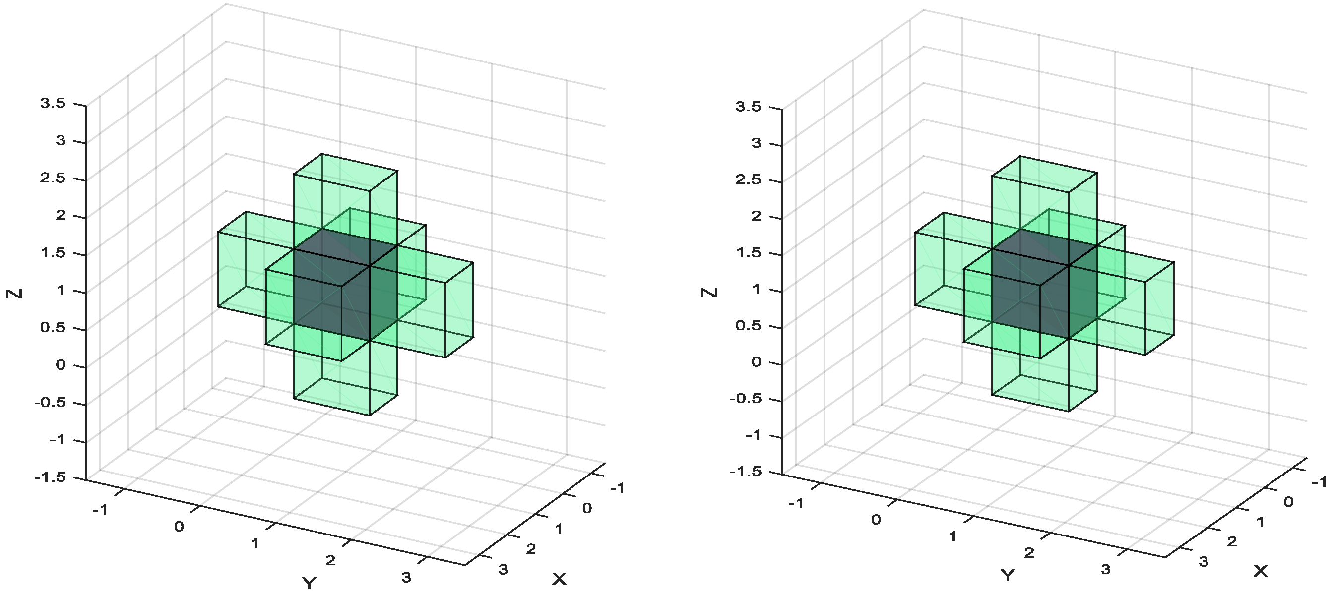
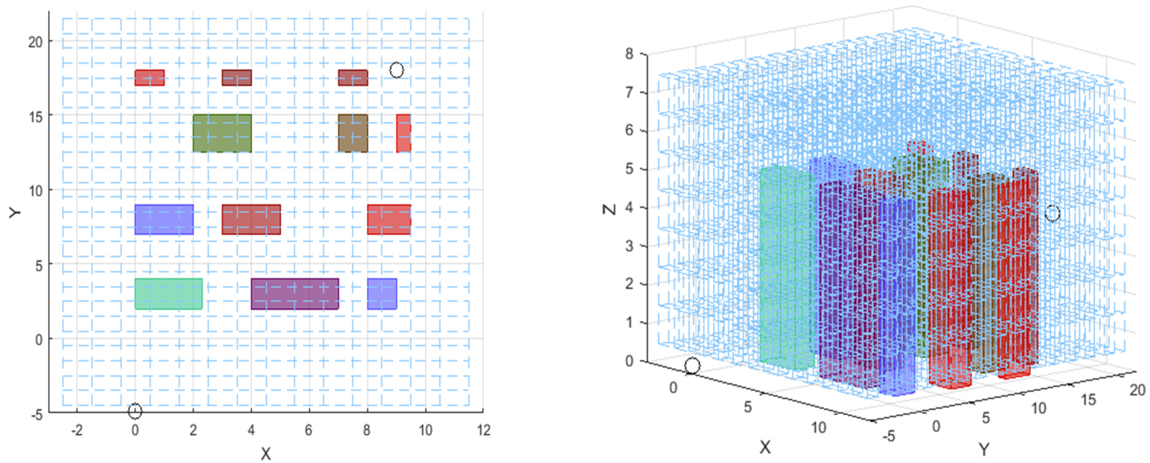
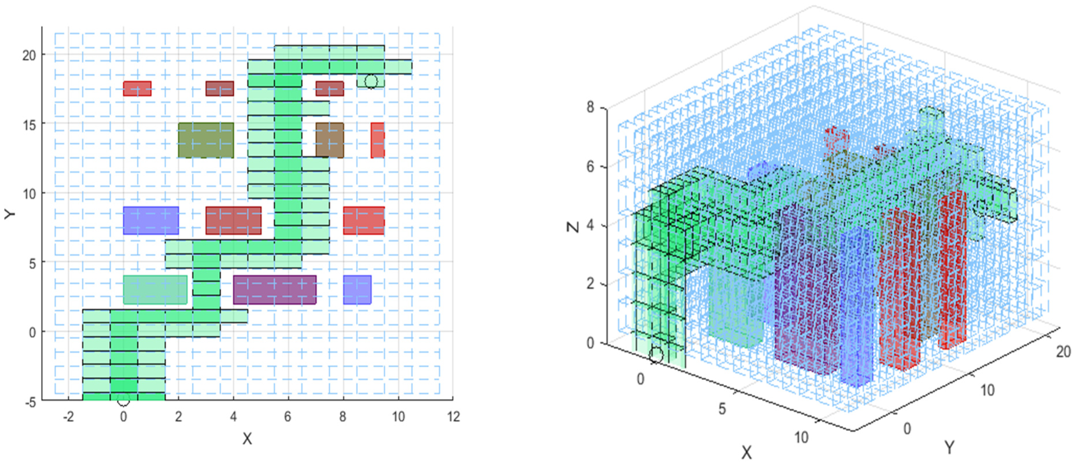
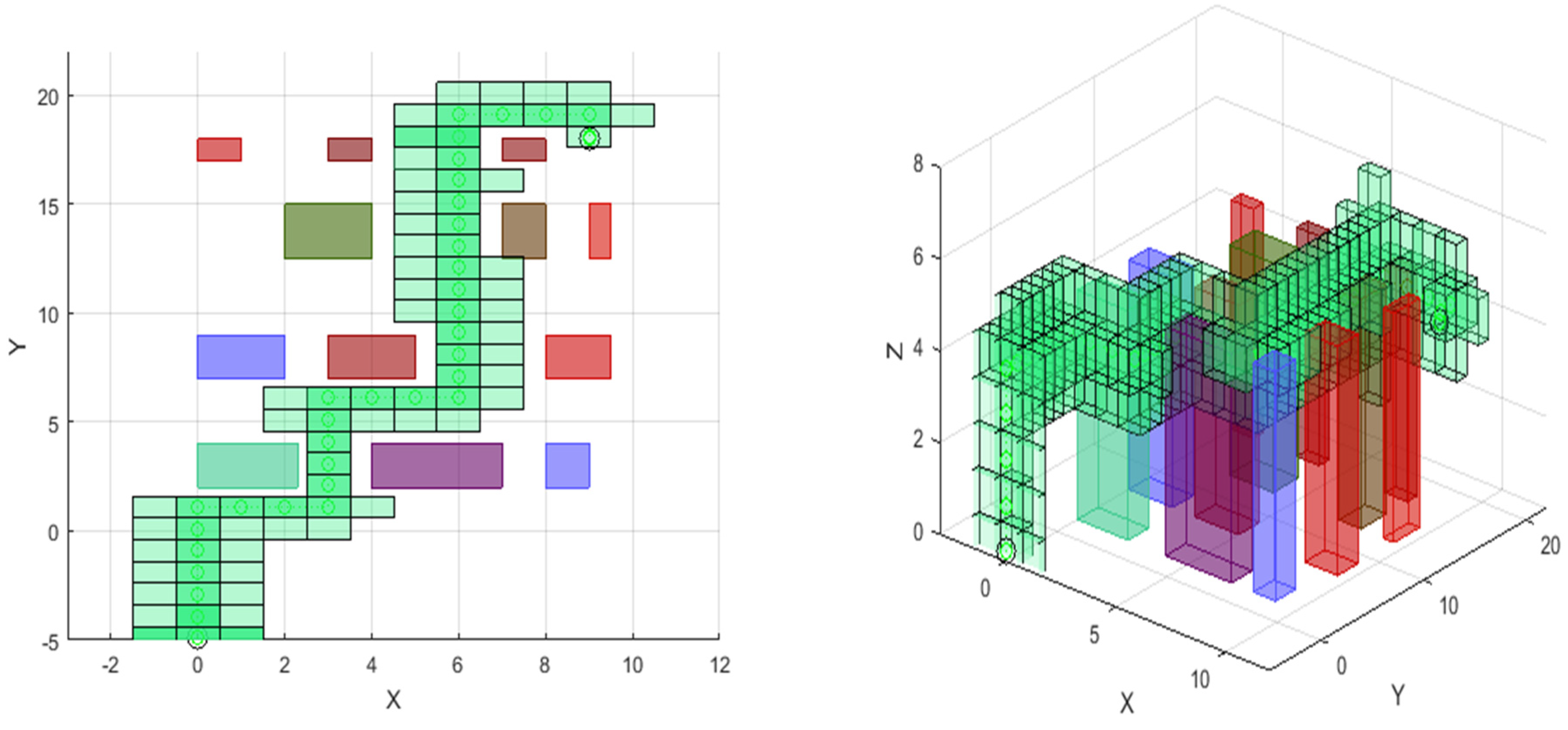
3.1. Three−Dimensional Path Search Using Modified A−Star Approach

Definition 1.

A heuristic refers to an estimate of the cost with the least value from any arbitrary current vertex to the goal vertex.

Mathematically, a simplified version of the heuristic function can be written as follows:

$$f\left(n\right)=g\left(n\right)+h\left(n\right)$$

(33)

where $g\left(n\right)$ is cost of the path from starting point to current node n, and $h\left(n\right)$ is the estimate of the cost from current node to goal node.

Remark 1.

In case, if $h\left(n\right)$ = 0, then only $g\left(n\right)$ plays a role in the algorithm, and A* is rendered to the Dijkstra algorithm. On the other hand, if the value of $h\left(n\right)$ is substantially large, the A* will behave like the greedy best-first search algorithm. The value of $h\left(n\right)$ plays a substantial role in expanding the nodes. If its value is relatively smaller, the algorithm will expand more nodes, which will make the path search slower. Contrarily, if its value is exactly equal to the cost of reaching from current vertex to goal, it finds the best and shortest possible path without expanding extra nodes. This ideality is difficult to achieve in three-dimensional (3D) cases, yet this algorithm is used in most applications due to its substantial fast path search ability.

In the abovementioned perspective, a heuristic is a method of providing the algorithm with some extra evaluative statistics in order to find a better path without thoroughly searching every possible vertex. The Dijkstra algorithm does not incorporate any heuristic function; it grows outwards from the start node and scans every vertex in the map to discover the shortest path. This is why it can be computationally expensive. Therefore, specifically for a 3D search problem, an admissible heuristic is central. In this work, the adopted heuristic relies on Euclidean distance estimation.

Definition 2.

A Euclidean heuristic gives a direct distance between current and goal points. For a three-dimensional case, it can be written as:

$$h=sqrt\lceil {\left(v_{x\left(n\right)}-v_{x\left(g\right)}\right)}^2+{\left(v_{y\left(n\right)}-v_{y\left(g\right)}\right)}^2+{\left(v_{z\left(n\right)}-v_{z\left(g\right)}\right)}^2\rceil$$

(34)

Another formalism known as the Manhattan heuristic gives summation of absolute differences in current and goal coordinates. For three-dimensional cases, we can write this mathematically as:

$$h=abs\left(v_{x\left(n\right)}-v_{x\left(g\right)}\right)+abs\left(v_{y\left(n\right)}-v_{y\left(g\right)}\right)+abs\left(v_{z\left(n\right)}-v_{z\left(g\right)}\right)$$

(35)

where $v_{i\left(n\right)}$ and $v_{i\left(g\right)}$ denote current and goal nodes, respectively.

Definition 3.

A heuristic function is known as monotone or consistent if its estimate for any current node is equal to or less than the estimated cost of reaching the goal from any neighbor of the current node plus the cost consumed in reaching that neighboring vertex from current node.

Mathematically, for any current node n and neighboring node i, we can write a consistent heuristic function as follows:

$$h\left(n\right)\le \mathrm{cost}\left(n,i\right)+h\left(i\right)$$

(36)

$$h\left(g\right)=0$$

(37)

where $\mathrm{cost}\left(n,i\right)$ is the step cost of reaching vertex i from n.

It is important to note that a heuristic function must essentially be admissible, i.e., it should never overestimate the cost of reaching the goal point. A consistent or monotonic function is always admissible. However, an admissible heuristic is not always consistent and therefore, it is made a consistent heuristic using the path-max equation as follows:

$$h^{\prime }\left(i\right)=\max \left(h\left(i\right), h\left(n\right)-\mathrm{cost}\left(n,i\right)\right)$$

(38)

An A* algorithm for three-dimensional path search is given in Algorithm 1. For 3D cases, it expands more nodes than the required ones and this ultimately increases the path length. Therefore, we have proposed another algorithm to cope with this problem in order to generate an accurate and shortest possible path.

In Algorithm 1, fewer than six vertices have been visited in the neighborhood of the current vertex in determining the next vertex on the route. This strategy allows us to restrain the search algorithm from entering into a long computational mode, as there is a possibility of visiting diagonal vertices in the neighborhood of current vertex. Diagonal search will enable us to find a path that is closer to the exact solution, i.e., the shortest possible path, at the cost of higher computation. However, paying a higher computational cost does not guarantee an exact solution to our problem. Contrarily, nondiagonal searching affects the searched path substantially, but a tradeoff has been determined between computational cost and extra nodes. The computed path generated by the search algorithm is not fully optimal and not even the shortest one. This can be seen in Figure 3, where path ABCD searched by the augmented A* is not the shortest; path ACD is shorter compared to path ABCD. After further iterations, we see that we can construct another route (the path AD) which is the shortest one. The feasibility of all these iterated paths has been checked via a collision detection algorithm (Algorithm 2) presented subsequently. Performing so few iterations can provide an even shorter path, and we can skip some of the extra path nodes. For this purpose, we have developed a truncation algorithm (Algorithm 3). Refined path nodes can then be connected using any interpolation method. Any order of the polynomial can be used for the purpose just conferred depending on the dynamical constraints of the quadrotor [44]. We, in this work, have used differential flatness theory to build the smooth trajectory.

Algorithm 1 A* algorithm for three-dimensional path search (with 6-sided search).

1: Function P(n) = Astar3D(3D_Environment, start, goal)

2: list_open = nodes to be evaluated; %initially only starting node is present

3: list_closed = nodes which have been examined; % initially empty

4: list_open (start_node) = 0;

5: while (list_open =! empty) do

6:  search the node with least f in list_open % the value of h(n) is same only for 6 neighbors, here one can plan the strategy for 18-sided search as well.

7:  n = node with least value of f;

8:  remove n from the list_open

9:  search the adj_cells of n  % adj_cells infer adjacent cells

10: for (each adj_cell)

% for three-dimensional case 6 adjacent cells have been visited in this work, however these can be up to 18 adjacent cells including the cells at the edges of a voxel holding the current vertex.

11:  if (adj_cell = goal) then

12:     stop the search

13:     adj_cell.g = n.g + dis_adj_cell;

14:     adj_cell.h = distance between adj_cell and goal;

15:     adj_cell.f = Adj_cell.g + Adj_cell.h;

16:  else if (node with same position as of adj_cell in list_open)

17:         if (node.f < adj_cell.f)

18:           skip adj_cell

19:         end if

20:  else if (node with same position as of adj_cell in list_closed)

21:         if (node.f < adj_cell.f)

21:           skip adj_cell

22:         else

23:           add node to list_open

24:         end if

25: end if

26: end for loop

27: add n to list_closed

28: end while

29: P(n)= list_closed

30: return P(n)

31: end function

Obstacles cluttered in a three-dimensional environment can be defined as follows:

$$\left[{\mathsf{\eta }}_{xyz}\right]=\left[\begin{array}{ccc}{\mathsf{\eta }}_x& {\mathsf{\eta }}_y& {\mathsf{\eta }}_z\end{array}\right]$$

(39)

where ${\left[{\mathsf{\eta }}_{xyz}\right]}_{min}={\left[\begin{array}{ccc}{\mathsf{\eta }}_x& {\mathsf{\eta }}_y& {\mathsf{\eta }}_z\end{array}\right]}_{min}$ and ${\left[{\mathsf{\eta }}_{xyz}\right]}_{max}={\left[\begin{array}{ccc}{\mathsf{\eta }}_x& {\mathsf{\eta }}_y& {\mathsf{\eta }}_z\end{array}\right]}_{max}$ represent lower and upper boundaries of obstacles in a three-dimensional environment, respectively.

The lower values of safe margins corresponding to lower boundaries can be calculated as follows:

$$\left[S_{min}\right]={\left[\begin{array}{ccc}{\mathsf{\eta }}_x& {\mathsf{\eta }}_y& {\mathsf{\eta }}_z\end{array}\right]}_{min}-\left[\begin{array}{ccc}{\delta }_x& {\delta }_y& {\delta }_z\end{array}\right]-\left[\begin{array}{ccc}{\mathsf{\Gamma }}_x& {\mathsf{\Gamma }}_y& {\mathsf{\Gamma }}_z\end{array}\right]$$

(40)

Similarly, upper safe margins are

$$\left[S_{max}\right]={\left[\begin{array}{ccc}{\mathsf{\eta }}_x& {\mathsf{\eta }}_y& {\mathsf{\eta }}_z\end{array}\right]}_{max}+\left[\begin{array}{ccc}{\delta }_x& {\delta }_y& {\delta }_z\end{array}\right]+\left[\begin{array}{ccc}{\mathsf{\Gamma }}_x& {\mathsf{\Gamma }}_y& {\mathsf{\Gamma }}_z\end{array}\right]$$

(41)

where $\left[\begin{array}{ccc}{\delta }_x& {\delta }_y& {\delta }_z\end{array}\right]$ denotes safety margins, which must be kept between the UAV and the obstacles during flight, while $\left[\begin{array}{ccc}{\mathsf{\Gamma }}_x& {\mathsf{\Gamma }}_y& {\mathsf{\Gamma }}_z\end{array}\right]$ is UAV size.

The boundary of the three-dimensional environment can be defined as $\left[B_{xyz}\right]=\left[\begin{array}{ccc}{B}_x& B_y& B_z\end{array}\right]$. The lower and upper boundaries of the three-dimensional environment can be written as ${\left[B_{xyz}\right]}_{min}={\left[\begin{array}{ccc}{B}_x& B_y& B_z\end{array}\right]}_{min}$ and ${\left[B_{xyz}\right]}_{max}={\left[\begin{array}{ccc}{B}_x& B_y& B_z\end{array}\right]}_{max}$, respectively.

Lemma 1.

If $\left[\begin{array}{ccc}{C}_x\left(n\right)& C_y\left(n\right)& C_z\left(n\right)\end{array}\right]$ is greater than or equal to $\left[S_{min}\right]$ and $\left[\begin{array}{ccc}{C}_x\left(n\right)& C_y\left(n\right)& C_z\left(n\right)\end{array}\right]$ is less than or equal to $\left[S_{max}\right]$, the collision will occur. $\left[\begin{array}{ccc}{C}_x\left(n\right)& C_y\left(n\right)& C_z\left(n\right)\end{array}\right]$ represents the coordinates of current vertex.

Lemma 2.

If the coordinates of current vertex $\left[\begin{array}{ccc}{C}_x\left(n\right)& C_y\left(n\right)& C_z\left(n\right)\end{array}\right]$ are less than the lower boundaries of the three-dimensional environment coordinates ${\left[B_{xyz}\right]}_{min}$, the collision will occur.

Lemma 2 specifically defines the limits of the environment. A UAV is considered in collision if it is outside the lower limits of the environment. Therefore, a mission is considered successful only when a UAV stays inside its defined environment.

Lemma 3.

If current vertex $\left[\begin{array}{ccc}{C}_x\left(n\right)& C_y\left(n\right)& C_z\left(n\right)\end{array}\right]$ is greater than the upper boundaries of the environment ${\left[B_{xyz}\right]}_{max}$, the collision will occur.

With the exceptions of Lemmas 1–3, the collision will not take place. Therefore, it is necessary for any safe flight of quadrotor UAV in a three-dimensional obstacle-cluttered environment to not lie among the abovementioned lemmas. Based on these lemmas, a collision detection algorithm is presented in Algorithm 2.

Algorithm 2 Collision detection algorithm.

1: input (3D_Environment, current vertex)

2: E = 3D Environment;

3: C(n) = current vertex;

4: E_min = min(E.obstacles);   %lower boundary of the obstacles

5: E_max = max(E.obstacles);    %upper boundary of the obstacles

6: minEo = E_min – margins – UAV_size;

7: maxEo = E.max + margins + UAV_size;

8: minEb = lower boundary of 3D Environment;

9: maxEb = upper boundary of 3D Environment;

10: if (Cx(n), Cy(n), Cz(n) ≥ minEo && Cx(n), Cy(n), Cz(n) ≤ maxEo)

11:         return collision;

12:  else if (Cx(n), Cy(n), Cz(n) < minEb)

13:         return collision;

14:  else if (Cx(n), Cy(n), Cz(n) > maxEb)

15:         return collision;

16:  else

17:         return collision_free;

18: End if

The rule of selecting the nodes, which constitutes the shortest path from the nodes explored by the heuristic search algorithm, follows the equation:

$$dP=p\left(k\right)-p\left(k-1\right)$$

(42)

where $dP$ denotes distance between the consecutive nodes, $p\left(k\right)$ is the current node and $p\left(k-1\right)$ is the previous node.

Remark 2.

If $dP$ follows either of the three lemmas mentioned previously, the node $p\left(k-1\right)$ lies on the shortest path and hence will be used to generate the shortest trajectory.

Remark 3.

If $dP$ does not follow any of the three lemmas, the next node on the list provided by the heuristic search algorithm will be examined using $dP=p\left(k\right)-p\left(k-1\right)$.

Based on Equation (42), Remarks 2 and 3, the proposed algorithm is presented as Algorithm 3. This algorithm will truncate the extra nodes of the path that has previously been obtained using the conventional A* algorithm. This proposed algorithm modifies the conventional approach of the A* algorithm and produces the shortest possible path in three-dimensional scenarios.

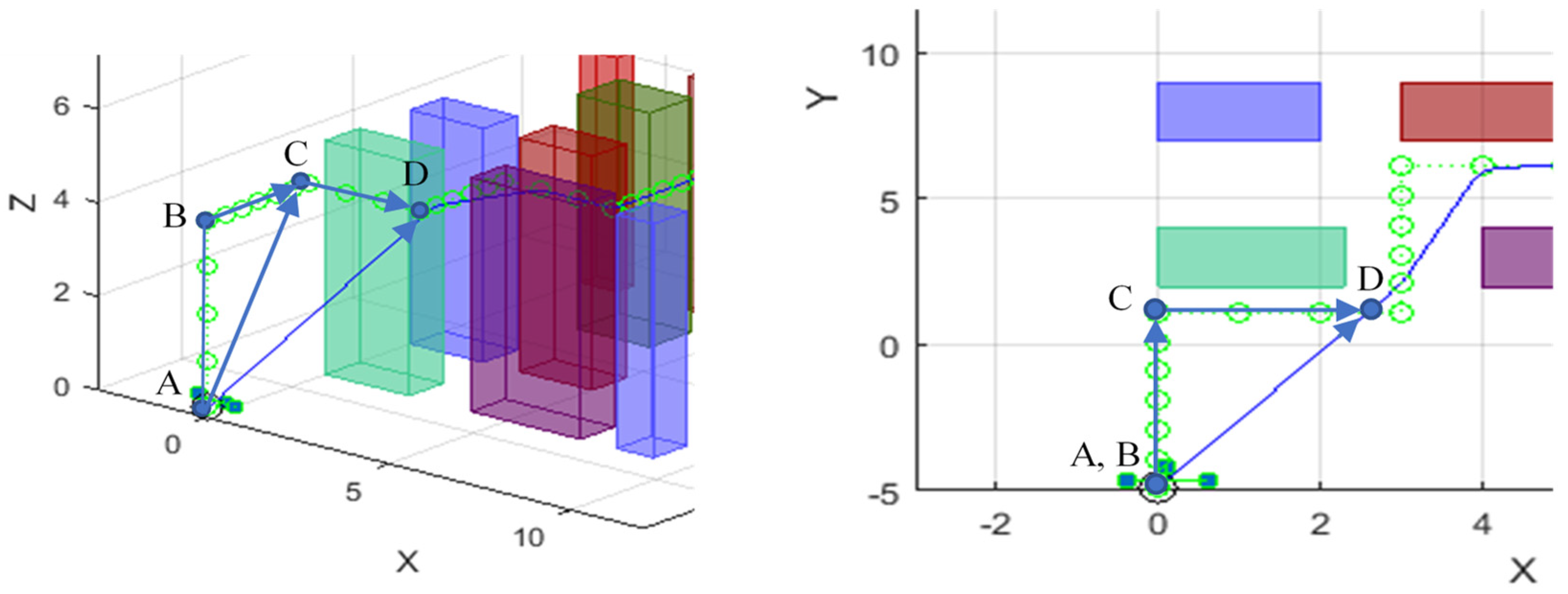
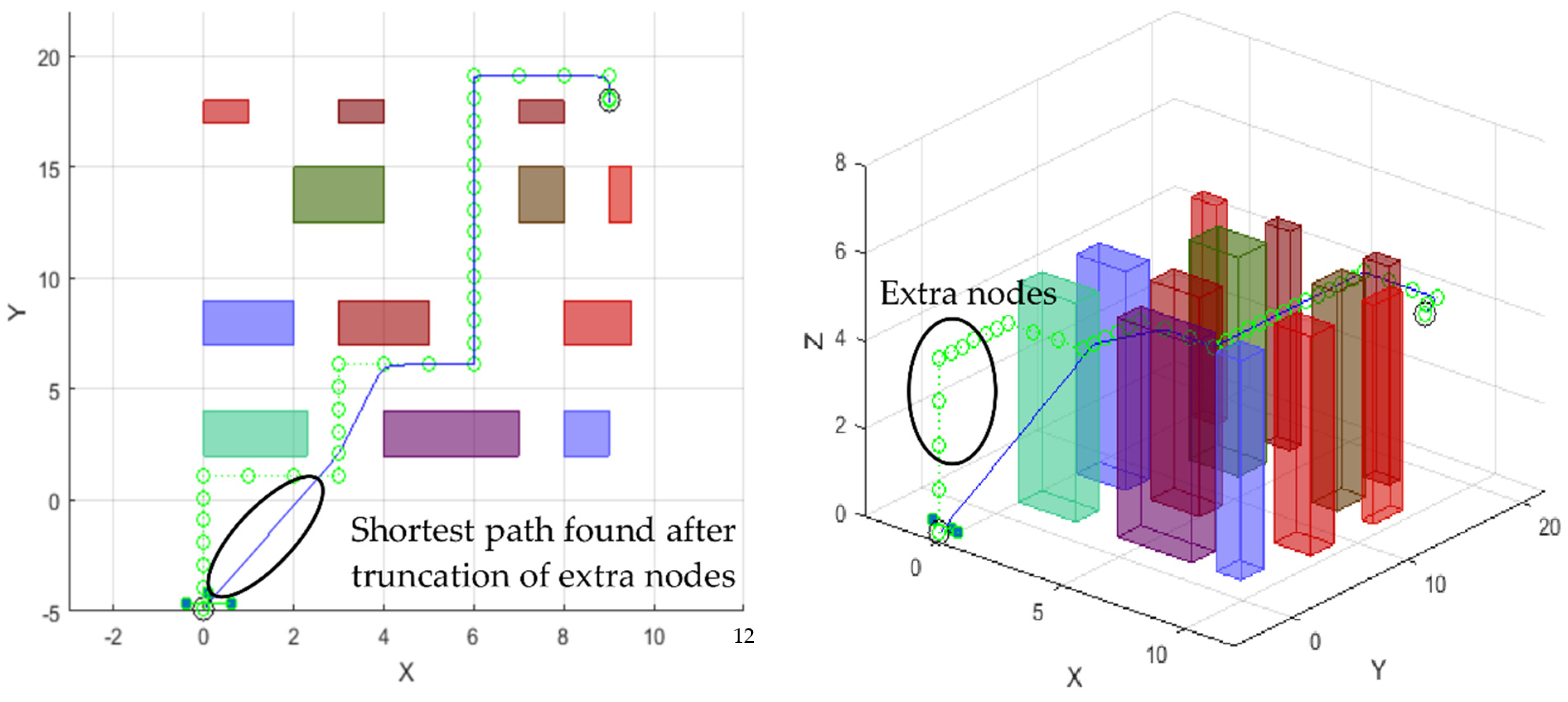
Algorithm 3 Proposed algorithm to refine the path obtained from conventional A* approach

1: function truncated_path = truncation(3D_Environment, P(n))

2: Truncated_path = P(1);

3: E.obstacles = 3D_Environment.obstacles;

4: for i = 2: length of path

5:     P = P(i) − P(1);

6:     if (collision between E.obstacles and P)

7:       Truncated _path = P(i − 1) % store the node explored just before collision-node into the truncated path list.

8:     else if (i == length of path)

9:       Truncated _path = P(i); % store last node in the truncated list

10:     else

11:       continue;

12:     end if

13: end for loop

3.2. Trajectory Generation

For optimal trajectory generation, the following functional can be used:

$$\chi \left(t\right)=argmi{n}_{\left(x\left(t\right)\right)}\underset{0}{\overset{T}{{\displaystyle \int }}}ℒ\left(x^n,x^{n-1}, x^{n-2},\dots \dots ,\dot{x},x,t\right).dt$$

(43)

In order to generate optimal trajectory $\chi \left(t\right)$, the following Euler–Lagrange equation must be satisfied:

$$\frac{\partial ℒ}{\partial x}-\frac{d}{dt}\left(\frac{\partial ℒ}{\partial \dot{x}}\right)+\frac{d^2}{d{t}^2}\left(\frac{\partial ℒ}{\partial \ddot{x}}\right)+\dots +{\left(-1\right)}^n\frac{d^n}{d{t}^n}\left(\frac{\partial ℒ}{\partial x^{\left(n\right)}}\right)=0$$

(44)

For a quadrotor UAV, n = 4 inputs create a fourth-order system with x and y states, and this can be proved by the following differential flatness theorem.

Theorem 1.

The inputs of the quadrotor are the function of selected flat outputs and their derivatives.

Proof of Theorem 1.

Recalling translational states from Equation (9) and assuming the linearized equation as:

$$m\ddot{x}=\left(\theta \cos \psi +\varphi \sin \psi \right)U_1$$

(45)

$$m\ddot{y}=\left(\theta \sin \psi -\varphi \cos \psi \right)U_1$$

(46)

$$\ddot{z}=-g+\left(\cos \varphi \cos \theta \right)\frac{1}{m}{U}_1$$

(47)

The fourth derivative is taken as:

$$\begin{array}{ll}m{x}^{\left(iv\right)}=& (\theta cos\psi +\varphi \sin \psi ){\ddot{U}}_1+2(\dot{\theta }\cos \psi -\theta \sin \psi \dot{\psi }+\dot{\varphi }\sin \psi +\varphi \cos \psi \dot{\psi }){\dot{U}}_1\\ & +(\ddot{\theta }\cos \psi -\dot{\theta }\sin \psi \dot{\psi }-\theta \sin \psi \ddot{\psi }-\theta \cos \psi {\dot{\psi }}^2+\ddot{\varphi }\sin \psi \\ & +\dot{\varphi }\cos \psi \dot{\psi }+\varphi \cos \psi \ddot{\psi }-\varphi \sin \psi {\dot{\psi }}^2)U_1\end{array}$$

(48)

$$\begin{array}{ll}m{y}^{\left(iv\right)}=& (\theta sin\psi -\varphi \cos \psi ){\ddot{U}}_1+2(\dot{\theta }\sin \psi +\theta \cos \psi \dot{\psi }-\dot{\varphi }\cos \psi +\varphi \sin \psi \dot{\psi }){\dot{U}}_1\\ & +(\ddot{\theta }\sin \psi +\dot{\theta }\cos \psi \dot{\psi }+\theta \cos \psi \ddot{\psi }-\theta \sin \psi {\dot{\psi }}^2-\ddot{\varphi }\cos \psi \\ & +\dot{\varphi }\sin \psi \dot{\psi }+\varphi \sin \psi \ddot{\psi }+\varphi cos\psi {\dot{\psi }}^2)U_1\end{array}$$

(49)

$$\begin{array}{ll}m{z}^{\left(iv\right)}=& -2(\dot{\theta }\cos \varphi \sin \theta +\dot{\varphi }\sin \varphi \cos \theta ){\dot{U}}_1+2(\dot{\varphi }\dot{\theta }\sin \varphi \sin \theta )U_1\\ & -({\dot{\varphi }}^2+{\dot{\theta }}^2)U_1\cos \varphi \cos \theta +(\cos \varphi \cos \theta ){\ddot{U}}_1\\ & -(\ddot{\varphi }\sin \varphi \cos \theta +\ddot{\theta }\cos \varphi \sin \theta )U_1\end{array}$$

(50)

Simplifying the rotational dynamics of quadrotor from Equation (10), we have:

$$\begin{array}{l}\ddot{\varphi }=\frac{l}{I_x}{U}_2\\ \ddot{\theta }=\frac{l}{I_y}{U}_3\\ \ddot{\psi }=\frac{1}{I_z}{U}_4\end{array}\}$$

(51)

For brevity, normalizing the inertial and length terms in Equation (51), we find a direct relation between the inputs and angular acceleration states. From Equations (48)–(51), we can write:

$$\begin{array}{r}m\lceil \begin{array}{c}{x}^{\left(iv\right)}\\ y^{\left(iv\right)}\\ z^{\left(iv\right)}\end{array}\rceil =\lceil \begin{array}{c}\left(-\dot{\theta }\sin \psi \dot{\psi }-\theta \cos \psi {\dot{\psi }}^2+\dot{\varphi }\cos \psi \dot{\psi }-\varphi \sin \psi {\dot{\psi }}^2\right)U_1+2\left(\dot{\theta }\cos \psi -\theta \sin \psi \dot{\psi }+\dot{\varphi }\sin \psi +\varphi \cos \psi \dot{\psi }\right){\dot{U}}_1\\ \left(\dot{\theta }\cos \psi \dot{\psi }-\theta \sin \psi {\dot{\psi }}^2+\dot{\varphi }\sin \psi \dot{\psi }+\varphi \cos \psi {\dot{\psi }}^2\right)U_1+2\left(\dot{\theta }\sin \psi +\theta \cos \psi \dot{\psi }-\dot{\varphi }\cos \psi +\varphi \sin \psi \dot{\psi }\right){\dot{U}}_1\\ \left(2\right(\dot{\varphi }\dot{\theta }\sin \varphi \sin \theta )-({\dot{\varphi }}^2+{\dot{\theta }}^2\left)\cos \varphi \cos \theta \right)U_1-2(\dot{\theta }\cos \varphi \cos \theta +\dot{\varphi }\sin \varphi \cos \theta ){\dot{U}}_1\end{array}\rceil \\ +\lceil \begin{array}{cccc}\left(\theta \cos \psi +\varphi \sin \psi \right)& \sin \psi & \cos \psi & \left(-\theta \sin \psi +\varphi \cos \psi \right)\\ \left(\theta \sin \psi -\varphi \cos \psi \right)& -\cos \psi & \sin \psi & \left(\theta \cos \psi +\varphi \sin \psi \right)\\ \cos \varphi \cos \theta & -\left(\sin \varphi \cos \theta \right)U_1& -\left(\cos \varphi \sin \theta \right)U_1& 0\end{array}\rceil \lceil \begin{array}{c}{\ddot{U}}_1\\ U_2\\ U_3\\ U_4\end{array}\rceil \end{array}$$

(52)

The translational states of the quadrotor create a fourth-order system; therefore, the control input directly relates to the snap of the position states. This completes the proof of Theorem 1. □

In order to achieve minimum control effort, we must minimize the snap of the translational states. To attain the goal just mentioned, the optimal trajectory $\chi \left(t\right)$ will assume the following form:

$$\chi \left(t\right)=argmi{n}_{\left(x\left(t\right)\right)}\underset{0}{\overset{T}{{\displaystyle \int }}}ℒ\left(x^{\left(iv\right)},x^{\left(iii\right)},\ddot{x},\dot{x},x,t\right)·dt$$

(53)

where $ℒ\left(x^{\left(iv\right)},x^{\left(iii\right)},\ddot{x},\dot{x},x,t\right)·dt$ is equal to ${\left(x^{\left(iv\right)}\right)}^2·dt$ for minimum snap trajectory.

Now the Euler—Lagrange equation can be solved as:

$$\frac{\partial ℒ}{\partial x}-\frac{d}{dt}\left(\frac{\partial ℒ}{\partial \dot{x}}\right)+\frac{d^2}{d{t}^2}\left(\frac{\partial ℒ}{\partial \ddot{x}}\right)-\frac{d^3}{d{t}^3}\left(\frac{\partial ℒ}{\partial x^{\left(3\right)}}\right)+\frac{d^4}{d{t}^4}\left(\frac{\partial ℒ}{\partial x^{\left(4\right)}}\right)=0$$

(54)

This will yield the following condition:

$$x^{\left(viii\right)}=0$$

(55)

The solution of Equation (55) yields the optimal trajectory of the following form:

$$\chi \left(t\right)={\lambda }_0+{\lambda }_{1}t+{\lambda }_2{t}^2+\cdots +{\lambda }_m{t}^m\hspace{1em}\mathrm{where} m=7$$

(56)

The trajectory computed above is one-dimensional and serves only for one segment. However, for a quadrotor UAV, to perform an autonomous flight through obstacles, the dimensionality of the trajectory is four and includes $x\left(t\right), y\left(t\right), z\left(t\right),\psi \left(t\right)$. Moreover, for a shortest path search problem, there are usually n trajectory segments for n + 1 number of waypoints, including start and goal points. We can formulate a trajectory for multiple dimensions and multiple segments as:

$$p_i{\left(t\right)}_{x\left(t\right),y\left(t\right),z\left(t\right),\psi \left(t\right)}={\lambda }_{i0}+{\lambda }_{i1}t+{\lambda }_{i2}{t}^2+\cdots +{\lambda }_{im}{t}^m\hspace{1em}\forall i=0\cdots n \mathrm{and} m=7$$

(57)

$$p_i{\left(t\right)}_{x\left(t\right),y\left(t\right),z\left(t\right),\psi \left(t\right)}={\displaystyle \sum }_{j=0}^m{\lambda }_{ij}{t}^j$$

(58)

Using Equation (57), a complete trajectory can be formulated over various time slots as follows:

$$P{\left(t\right)}_{x\left(t\right),y\left(t\right),z\left(t\right),\psi \left(t\right)}=\{\begin{array}{cc}{\displaystyle {\displaystyle \sum }_{j=0}^m}{\lambda }_{0j}{t}^j& t_0\le t<t_1\hfill \\ {\displaystyle {\displaystyle \sum }_{j=0}^m}{\lambda }_{1j}{t}^j& t_1\le t<t_2\hfill \\ ⋮& \\ {\displaystyle {\displaystyle \sum }_{j=0}^m}{\lambda }_{nj}{t}^j& t_n\le t<t_{n+1}\hfill \end{array}$$

(59)

where $m$ defines the degree of polynomial.

To solve the coefficients of Equation (59), some constraints must inevitably be considered. These constraints are explained subsequently.

3.2.1. Constraints on Positions

For n + 1 intermediate points, there are usually n trajectory sections, and in this case, each trajectory section is represented by a seventh-order polynomial. These polynomials lie between intermediate points, and the positions of these points are well defined. Therefore, these polynomials must pass through these well-defined positions of the intermediate points at various allocated time stamps. Mathematically, we can write this as follows:

$$p_i\left(t_{i-1}\right)={\xi }_{i-1}$$

(60a)

$$p_i\left(t_i\right)={\xi }_i$$

(60b)

where $i=1\cdots n$, $t_{i-1}$ is the initial time and $t_i$ denotes the final time for ith polynomial, while the terms ${\xi }_{i-1}$ and ${\xi }_i$ are the initial and the final positions for ith polynomial, respectively.

3.2.2. Constraints on Derivatives

For the higher-ordered dynamics of the quadrotor, it is pertinent to guarantee smooth transitions at intermediate points from one trajectory section to the next. Therefore, in order to serve the purpose just mentioned, successive derivatives of adjacent polynomials at each intermediate point must be kept equal. The order of the plant dynamics defines the derivative indices that will ensure the smooth switching between adjacent trajectory sections.

$$p_{i-1}^{\left(k\right)}\left(t_i\right)=p_i^{\left(k\right)}\left(t_i\right)\hspace{1em}\mathrm{where} i=1\cdots n, \mathrm{and} \mathrm{for} m=7, 1\le k\le 4$$

(61)

3.2.3. Constraints on Start and Goal Points

In a trajectory of multiple segments, there are always start and goal points, and a quadrotor must be at rest in these points. Therefore, we can impose the constraints on these points with respect to the position of these points and their kth successive derivates.

$$p_i^{\left(k\right)}\left(0\right)=0$$

(62a)

$$p_i^{\left(k\right)}\left(t_n\right)=0$$

(62b)

where the derivative index is $0\le k\le 3$ for the seventh-degree polynomial.

Applying the abovementioned constraints to the nodes, which are obtained after the truncation process in the shortest path search problem, we can formulate the problem in the following form to calculate the coefficients of the optimal trajectory:

$${\mathsf{\lambda }}_{n\left(m+1\right)\times 1}=T_{n\left(m+1\right)\times n\left(m+1\right)}^{-1}·{\xi }_{n\left(m+1\right)\times 1}$$

(63)

where $\lambda$ is the coefficients’ matrix, $T$ is the time series matrix, and $\xi$ denotes defined values of positions and their successive derivatives.

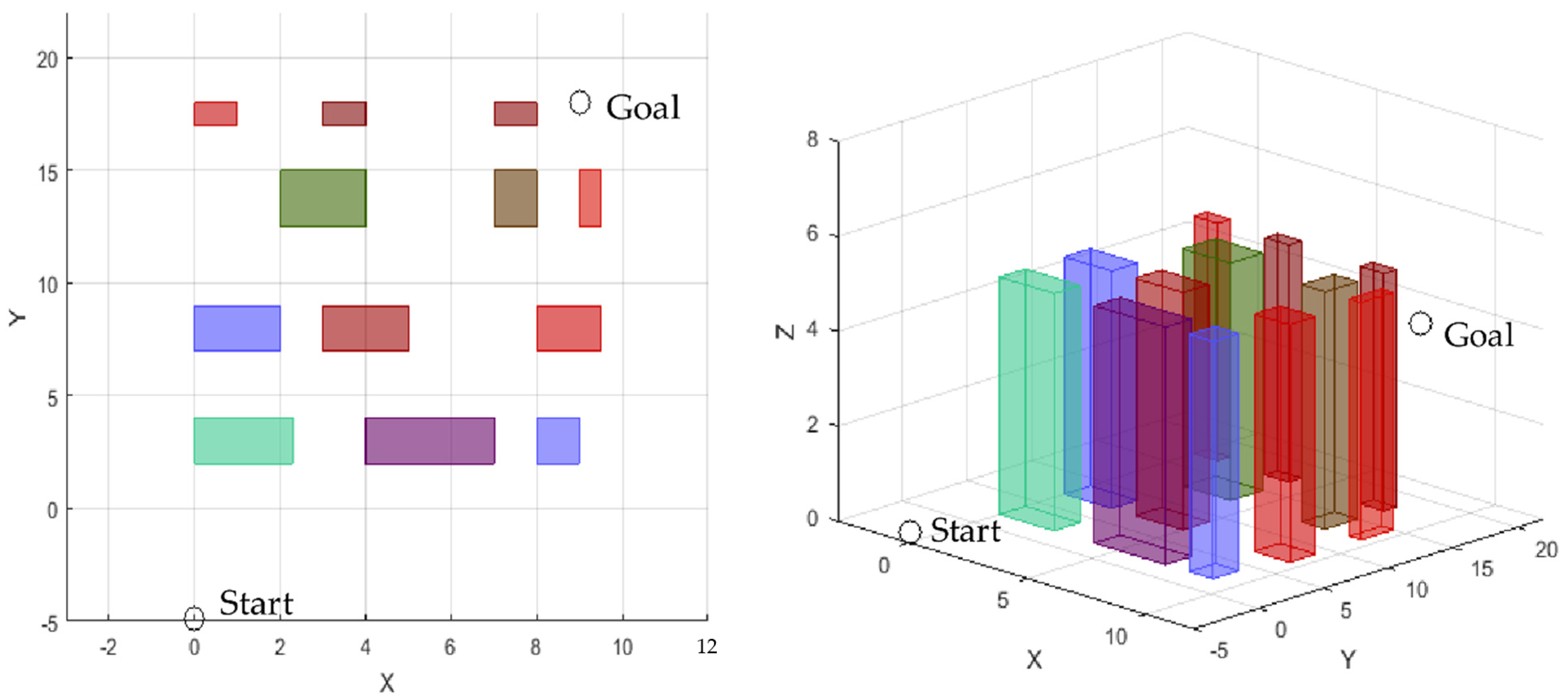
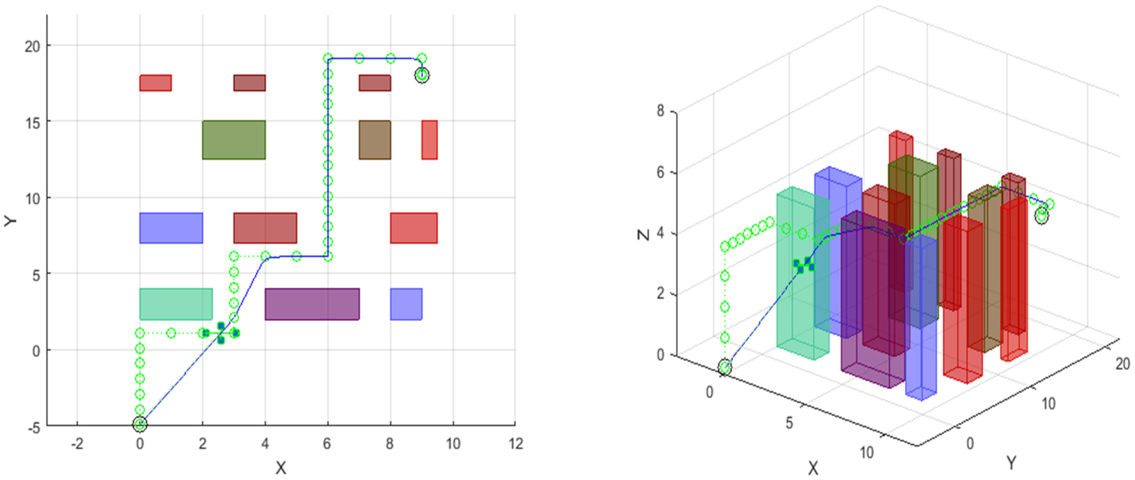
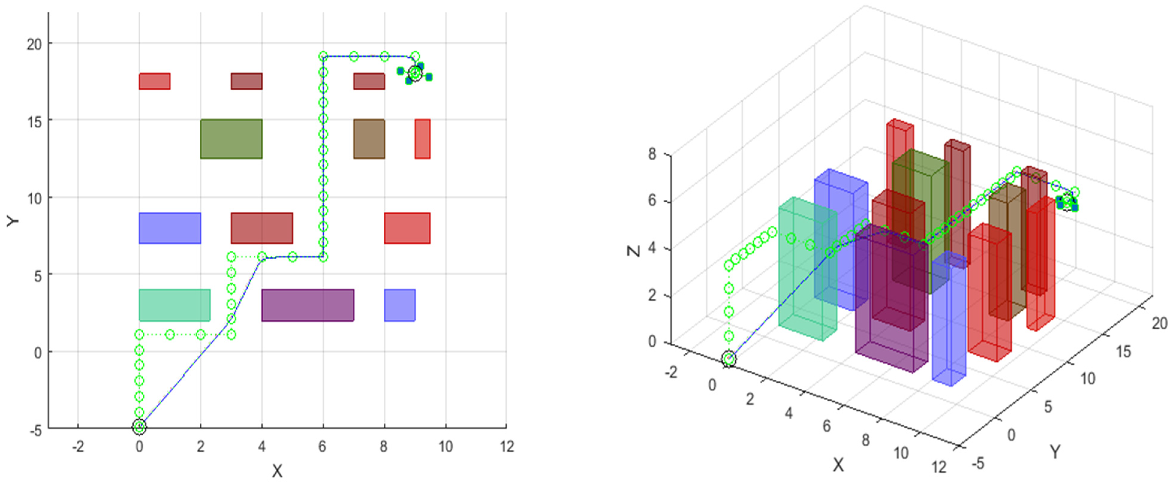
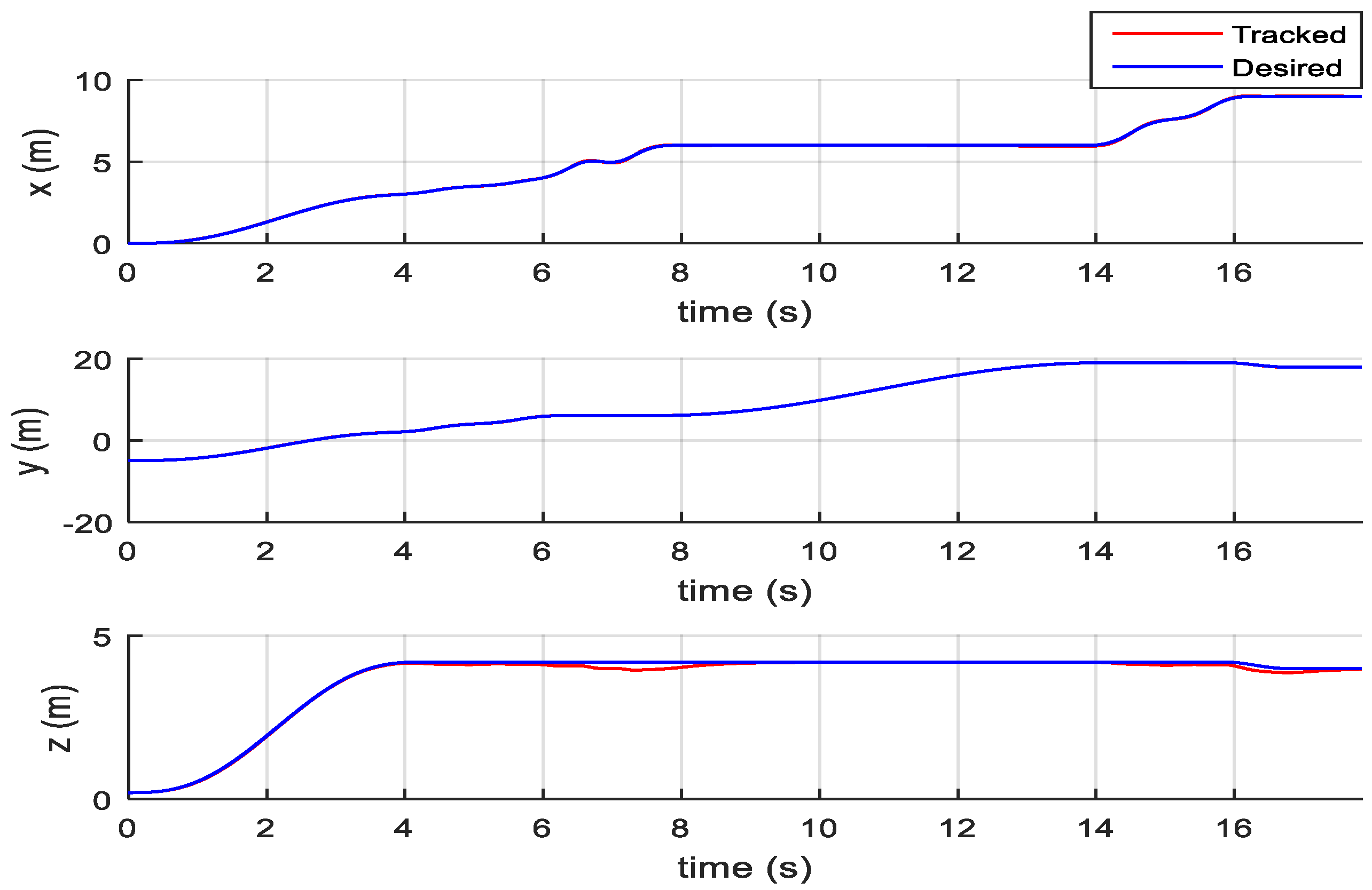
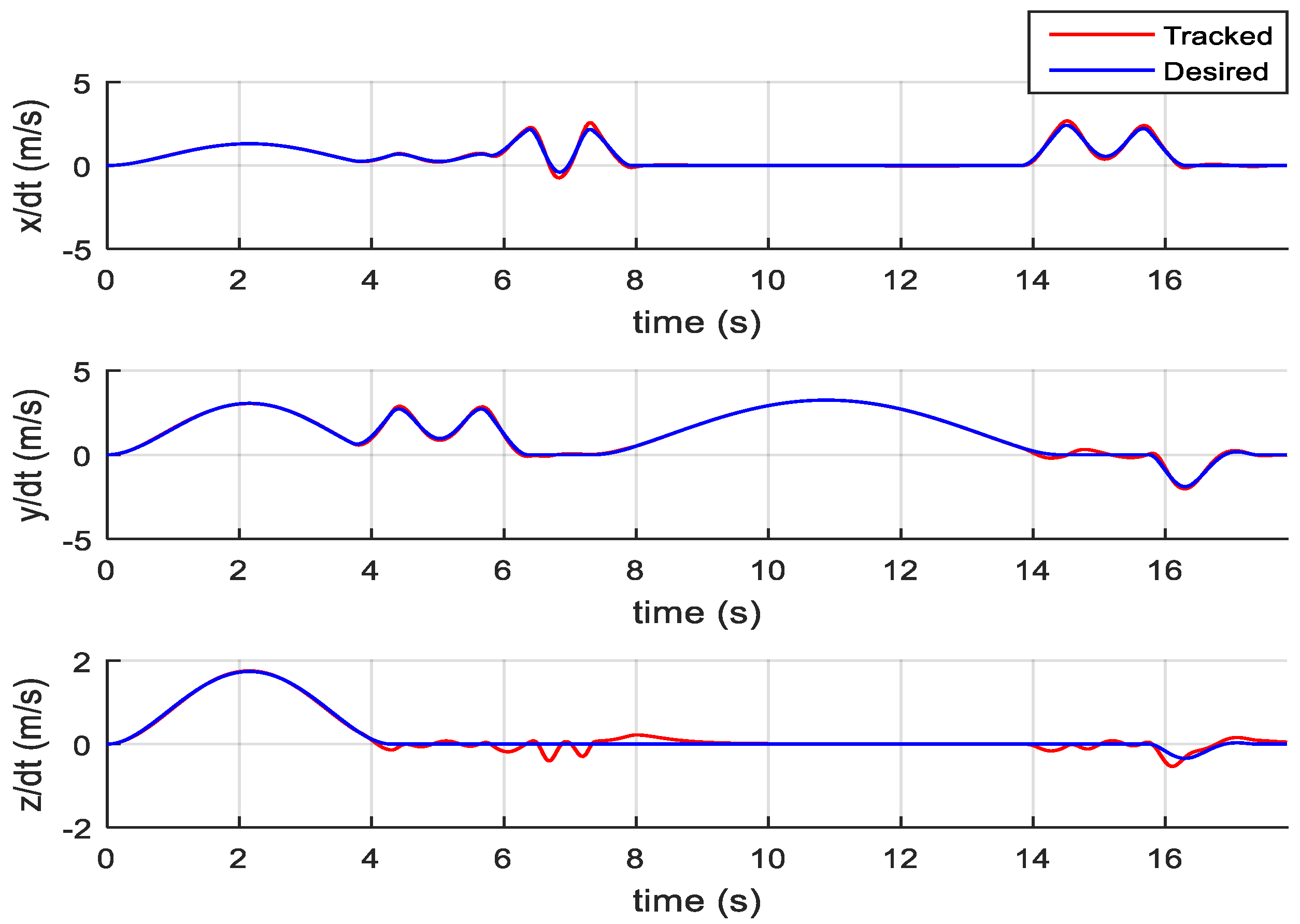
4. Simulations

This section presents the results of numerical simulations, and MATLAB is used to elaborate upon the findings and developments of this paper. Initially, the controller conferred earlier was developed along with the model of the quadrotor UAV in order to track the computed final trajectory. The model parameters and controller gains, that have been used in the simulation environment, are listed in

Table 1. Model parameters.

Parameter	Value	Unit
Mass (m)	0.2	kg
Arm length (l)	0.09	m
Inertia (Ix)	0.00026	kgm2
Inertia (Iy)	0.00026	kgm2
Inertia (Iz)	0.00040	kgm2
Gravity (g)	9.81	m/s2

and

Table 2. Controller gains.

Controller	Parameter	Value
Outer Loop Controller	$K_p$(x, y, z)	2
Outer Loop Controller	$K_d$(x, y, z)	1.4
Inner Loop Controller	$K_p$$(\varphi ,\theta ,\psi$)	7
Inner Loop Controller	$K_d$($\varphi ,\theta ,\psi$)	0.3

, respectively. Because any path search algorithm requires a map and start and goal points, a three-dimensional environment containing the obstacles was modelled in MATLAB. The concept of real-time tall buildings is used to model the obstacles. Subsequently, the start point and the goal point were defined in the constructed obstacle-cluttered environment. Figure 4 illustrates the 2D and 3D views of the environment. Before handing this map over to the search algorithm, meshing is performed, which divides the whole map into small, cubical, interconnected blocks. Mesh size is decisive in performing the computation. A relatively smaller mesh size would compute a more optimal and shorter path but would do so at the cost of heavy computational power. Figure 5 demonstrates the map environment with meshing. This map is handed over to the A* search algorithm, which subsequently finds a shorter path between start and goal points. Figure 6 shows the progression of the search algorithm in 2D and 3D views. The shortest path found by the augmented A* algorithm is illustrated in Figure 7, which shows 2D and 3D views.

Technically, after the completion of the algorithmic search, the path found is still not the optimized version. Specifically, in a three-dimensional case, the path can further be optimized depending on the situation. Moreover, the shortest path found after the truncation process contains infinite curvatures at the corner points and traversal of the path using any quadrotor UAV is rather challenging. This requires smoothing of these corner points by incorporating any higher-ordered polynomial. The fifth-order polynomial is used to shape these corner points to reduce the curvatures to a finite extent. Consequently, the found shortest path is optimized further by smoothing the corner points. The 2D and 3D views of this process can be seen in Figure 8.

The final version of the generated trajectory is then given to the conferred flight controller as desired Cartesian commands. The controller successfully traverses the trajectory and steers the quadrotor UAV through the obstacle-cluttered space autonomously. The progression of trajectory traversal can be seen in Figure 9. After the follow-up of the desired trajectory, the quadrotor UAV successfully reaches the goal point, as shown in Figure 10. Finally, the controller performance is illustrated in Figure 11, where the desired and tracked Cartesian states of the model are displayed. The desired and tracked velocities are shown in Figure 12. The results verify the effectiveness and the promising formulation of the flight controller.

5. Conclusions

Motion-planning is central for any autonomous robotic system, and most of the search algorithmshave only been studied for two-dimensional applications in the literature. In this paper, a detailed implementation and design of a modified A* search algorithm for three-dimensional cases have been presented. With a conventional A* approach, 3D search poses the issue of exploration of extra nodes, which results in a suboptimal path. Such suboptimal paths render a trajectory that increases the control effort of the UAV and obviously reduces flight endurance. This issue has been solved by proposing a modified A* approach based on a truncation algorithm that renders the shortest possible path by removing extra nodes. To generate a dynamically feasible trajectory for a quadrotor, a detailed proof of differential flatness has been presented. Subsequently, path nodes obtained by the modified A* approach were further processed by a flatness-based trajectory generator in order to have a smooth and dynamically feasible trajectory, i.e., a trajectory with finite curvatures. The adopted modified approach significantly reduced the path length (see figures in the paper) and control effort of the UAV (as per the Euler–Lagrange constraints). This obviously enhances flight endurance. A micro quadrotor UAV model is then used to demonstrate the autonomous trajectory generation and tracking through cluttered obstacles in a three-dimensional space. This study can be further enhanced by incorporating other path-planning algorithms, e.g., potential gradient, D*, D-lite, etc.

References

- Farid, G.; Mo, H.; Ali, S.M.; Liwei, Q. A review on linear and nonlinear control techniques for position and attitude control of a quadrotor. Control. Intell. Syst. 2017, 45, 43–57. [Google Scholar]
- Kendoul, F. Survey of advances in guidance, navigation, and control of unmanned rotorcraft systems. J. Field Robot. 2012, 29, 315–378. [Google Scholar] [CrossRef]
- Liu, P.; Chen, A.Y.; Huang, Y.N.; Han, J.Y.; Lai, J.S.; Kang, S.C.; Wu, T.H.; Wen, M.C.; Tsai, M.H. A review of rotorcraft Unmanned Aerial Vehicle (UAV) developments and applications in civil engineering. Smart. Struct. Syst. 2014, 13, 1065–1094. [Google Scholar] [CrossRef]
- Özbek, N.S.; Önkol, M.; Efe, M.Ö. Feedback control strategies for quadrotor-type aerial robots: A survey. Trans. Inst. Meas. Control. 2016, 38, 529–554. [Google Scholar] [CrossRef]
- Zhang, X.; Li, X.; Wang, K.; Lu, Y. A Survey of Modelling and Identification of Quadrotor Robot. Abstr. Appl. Anal. 2014, 2014, 16. [Google Scholar] [CrossRef]
- Bullo, F.; Frazzoli, E.; Pavone, M.; Savla, K.; Smith, S.L. Dynamic Vehicle Routing for Robotic Systems. Proc. IEEE 2011, 99, 1482–1504. [Google Scholar] [CrossRef] [Green Version]
- Mo, H.; Farid, G. Nonlinear and adaptive intelligent control techniques for quadrotor UAV—A survey. Asian J. Control 2019, 21, 989–1008. [Google Scholar] [CrossRef]
- Tokekar, P.; Hook, J.V.; Mulla, D.; Isler, V. Sensor planning for a symbiotic UAV and UGV system for precision agriculture. In Proceedings of the 2013 IEEE/RSJ International Conference on Intelligent Robots and Systems, Tokyo, Japan, 3–7 November 2013; pp. 5321–5326. [Google Scholar]
- Alexis, K.; Nikolakopoulos, G.; Tzes, A. On Trajectory Tracking Model Predictive Control of an Unmanned Quadrotor Helicopter Subject to Aerodynamic Disturbances. Asian J. Control 2014, 16, 209–224. [Google Scholar] [CrossRef]
- Besnard, L.; Shtessel, Y.B.; Landrum, B. Quadrotor vehicle control via sliding mode controller driven by sliding mode disturbance observer. J. Frankl. Inst. 2012, 349, 658–684. [Google Scholar] [CrossRef]
- Ghommam, J.; Charland, G.; Saad, M. Three-Dimensional Constrained Tracking Control Via Exact Differentiation Estimator of a Quadrotor Helicopter. Asian J. Control 2015, 17, 1093–1103. [Google Scholar] [CrossRef]
- Lee, D.; Jin Kim, H.; Sastry, S. Feedback linearization vs. adaptive sliding mode control for a quadrotor helicopter. Int. J. Control Autom. Syst. 2009, 7, 419–428. [Google Scholar] [CrossRef]
- Mellinger, D.; Michael, N.; Kumar, V. Trajectory generation and control for precise aggressive maneuvers with quadrotors. Int. J. Robot. Res. 2012, 31, 664–674. [Google Scholar] [CrossRef]
- Xiong, J.-J.; Zhang, G. Discrete-time sliding mode control for a quadrotor UAV. Int. J. Light Electron Opt. 2016, 127, 3718–3722. [Google Scholar] [CrossRef]
- Zou, Y. Nonlinear robust adaptive hierarchical sliding mode control approach for quadrotors. Int. J. Robust Nonlinear Control 2017, 27, 925–941. [Google Scholar] [CrossRef]
- Chen, Y.-b.; Luo, G.-c.; Mei, Y.-s.; Yu, J.-q.; Su, X.-l. UAV path planning using artificial potential field method updated by optimal control theory. Int. J. Syst. Sci. 2016, 47, 1407–1420. [Google Scholar] [CrossRef]
- Duchoň, F.; Babinec, A.; Kajan, M.; Beňo, P.; Florek, M.; Fico, T.; Jurišica, L. Path Planning with Modified a Star Algorithm for a Mobile Robot. Procedia Eng. 2014, 96, 59–69. [Google Scholar] [CrossRef] [Green Version]
- Foead, D.; Ghifari, A.; Kusuma, M.B.; Hanafiah, N.; Gunawan, E. A Systematic Literature Review of A* Pathfinding. Procedia Comput. Sci. 2021, 179, 507–514. [Google Scholar] [CrossRef]
- Tang, G.; Tang, C.; Claramunt, C.; Hu, X.; Zhou, P. Geometric A-Star Algorithm: An Improved A-Star Algorithm for AGV Path Planning in a Port Environment. IEEE Access 2021, 9, 59196–59210. [Google Scholar] [CrossRef]
- Zheng, T.; Xu, Y.; Zheng, D. AGV Path Planning based on Improved A-star Algorithm. In Proceedings of the 2019 IEEE 3rd Advanced Information Management, Communicates, Electronic and Automation Control Conference (IMCEC), Chongqing, China, 11–13 October 2019; pp. 1534–1538. [Google Scholar]
- Erke, S.; Bin, D.; Yiming, N.; Qi, Z.; Liang, X.; Dawei, Z. An improved A-Star based path planning algorithm for autonomous land vehicles. Int. J. Adv. Robot. Syst. 2020, 17, 1729881420962263. [Google Scholar] [CrossRef]
- Ghaffari, A. An Energy Efficient Routing Protocol for Wireless Sensor Networks using A-star Algorithm. J. Appl. Res. Technol. 2014, 12, 815–822. [Google Scholar] [CrossRef] [Green Version]
- Castillo-García, P.; Muñoz Hernandez, L.E.; García Gil, P. Chapter 9—Trajectory Generation, Planning &Tracking. In Indoor Navigation Strategies for Aerial Autonomous Systems; Butterworth-Heinemann: Oxford, UK, 2017; pp. 213–241. [Google Scholar]
- Wang, G.-G.; Chu, H.E.; Mirjalili, S. Three-dimensional path planning for UCAV using an improved bat algorithm. Aerosp. Sci. Technol. 2016, 49, 231–238. [Google Scholar] [CrossRef]
- Chen, Y.; Mei, Y.; Yu, J.; Su, X.; Xu, N. Three-dimensional unmanned aerial vehicle path planning using modified wolf pack search algorithm. Neurocomputing 2017, 266, 445–457. [Google Scholar] [CrossRef]
- Contreras-Cruz, M.A.; Ayala-Ramirez, V.; Hernandez-Belmonte, U.H. Mobile robot path planning using artificial bee colony and evolutionary programming. Appl. Soft. Comput. 2015, 30, 319–328. [Google Scholar] [CrossRef]
- Liang, Y.; Juntong, Q.; Xiao, J.; Xia, Y. A literature review of UAV 3D path planning. In Proceedings of the 11th World Congress on Intelligent Control and Automation, Shenyang, China, 29 June–4 July 2014; pp. 2376–2381. [Google Scholar]
- Lu, Y.; Xue, Z.; Xia, G.-S.; Zhang, L. A survey on vision-based UAV navigation. Geo-Spat. Inf. Sci. 2018, 21, 21–32. [Google Scholar] [CrossRef] [Green Version]
- Aggarwal, S.; Kumar, N. Path planning techniques for unmanned aerial vehicles: A review, solutions, and challenges. Comput. Commun. 2020, 149, 270–299. [Google Scholar] [CrossRef]
- Goerzen, C.; Kong, Z.; Mettler, B. A Survey of Motion Planning Algorithms from the Perspective of Autonomous UAV Guidance. J. Intell. Robot. Syst. 2009, 57, 65. [Google Scholar] [CrossRef]
- Zhao, Y.; Zheng, Z.; Liu, Y. Survey on computational-intelligence-based UAV path planning. Knowl. Based Syst. 2018, 158, 54–64. [Google Scholar] [CrossRef]
- Mac, T.T.; Copot, C.; Tran, D.T.; De Keyser, R. Heuristic approaches in robot path planning: A survey. Robot. Auton. Syst. 2016, 86, 13–28. [Google Scholar] [CrossRef]
- Goel, U.; Varshney, S.; Jain, A.; Maheshwari, S.; Shukla, A. Three Dimensional Path Planning for UAVs in Dynamic Environment using Glow-worm Swarm Optimization. Procedia Comput. Sci. 2018, 133, 230–239. [Google Scholar] [CrossRef]
- Kunchev, V.; Jain, L.; Ivancevic, V.; Finn, A. Path Planning and Obstacle Avoidance for Autonomous Mobile Robots: A Review. In Knowledge-Based Intelligent Information and Engineering Systems; Springer: Berlin/Heidelberg, Germany, 2006; pp. 537–544. [Google Scholar]
- Dadkhah, N.; Mettler, B. Survey of Motion Planning Literature in the Presence of Uncertainty: Considerations for UAV Guidance. J. Intell. Robot. Syst. 2012, 65, 233–246. [Google Scholar] [CrossRef]
- Cocuzza, S.; Doria, A. Modeling and Identification of Vibrations in a UAV for Aerial Manipulation. Mech. Mach. Sci. 2021, 91, 182–190. [Google Scholar] [CrossRef]
- Cocuzza, S.; Doria, A. Experimental vibration analysis and development of the dynamic model of a uav for aerial manipulation. Int. J. Mech. Control. 2021, 22, 71–81. [Google Scholar]
- Cocuzza, S.; Rossetto, E.; Doria, A. Dynamic interaction between robot and UAV in aerial manipulation. In Proceedings of the 2020 19th International Conference on Mechatronics—Mechatronika, Prague, Czech Republic, 2–4 December 2020. [Google Scholar] [CrossRef]
- Cocuzza, S.; Pretto, I.; Debei, S. Least-squares-based reaction control of space manipulators. J. Guid. Control. Dyn. 2012, 35, 976–986. [Google Scholar] [CrossRef]
- Tringali, A.; Cocuzza, S. Globally optimal inverse kinematics method for a redundant robot manipulator with linear and nonlinear constraints. Robotics 2020, 9, 61. [Google Scholar] [CrossRef]
- Tringali, A.; Cocuzza, S. Finite-horizon kinetic energy optimization of a redundant space manipulator. Appl. Sci. Switz. 2021, 11, 2346. [Google Scholar] [CrossRef]
- Cocuzza, S.; Menon, C.; Angrilli, F. Free-flying robot tested on ESA parabolic flights: Simulated microgravity tests and simulator validation. In Proceedings of the International Astronautical Federation—58th International Astronautical Congress, Hyderabad, India, 24–28 September 2007; Volume 1, pp. 593–608. [Google Scholar]
- Farid, G.; Mo, H.; Ahmed, M.I.; Ehsan, A. On control law partitioning for nonlinear control of a quadrotor UAV. In Proceedings of the 2018 15th International Bhurban Conference on Applied Sciences and Technology (IBCAST), Islamabad, Pakistan, 9–13 January 2018; pp. 257–262. [Google Scholar]
- Farid, G.; Hamid, H.T.; Karim, S.; Tahir, S. Waypoint-Based Generation of Guided and Optimal Trajectories for Autonomous Tracking Using a Quadrotor UAV. Stud. Inform. Control. 2018, 27, 223–234. [Google Scholar] [CrossRef]