Abstract
Due to their importance in representing, explaining, and analyzing phenomena, statistical lifetime distributions are widely used in science. As a result, this paper discusses a modern lifetime model called Birnbaum–Saunders logistic distribution. This distribution extends the Birnbaum–Saunders distribution, as it has proven to be characterized by great flexibility in data modeling in practice. Different features of this distribution have been discussed. The parameters of the model are estimated using the maximum likelihood and modified moment estimation methods. To evaluate the performance of the methods, a simulation study with data contamination scenarios is presented. Finally, the new model’s flexibility is tested using real datasets.
1. Introduction
Lifetime models are a probability distribution with either a non-negative or positive support which are considered in survival analysis. In the literature, there exist many well-known life models, including, but not limited to, the exponential distribution and its generalization; the Weibull distribution. The main limitation of these two models is that they are not suitable for data with non-monotonic hazard rates. Examples of non-monotonic hazard rates are the bathtub and the upside-down hazard rates. From a medical perspective, the bathtub hazard rate represents three life phases. The first phase is called the infant mortality period which is a duration of time with decreasing hazard rate. The second part is the normal life period in which a constant hazard rate is maintained. The final phase is a period of time in which the hazard rate increases due to aging. Additionally, the upside-down hazard rate can be considered to describe the behavior of malicious diseases, such as cancer. In fact, ref. [1] observed such a hazard rate in the case of a certain type of breast cancer. They concluded that the mortality (i.e., hazard) rate increased to its highest peak which was approximately three years after the cancer was diagnosed. Afterwards, they observed that over a specified amount of time, the mortality rate decreases slowly.
In the literature, skewed life distributions such as the inverse Gaussian, the log-Gaussian, and the Birnbaum–Saunders distribution have been used to model phenomena with an upside-down hazard rate [2]. The latter model, however, received considerable attention from many researchers due to its desirable properties and physical interpretation. In fact, at least 200 articles and a single study monograph have previously been published detailing many aspects and advancements connected to this lifetime model. For more details, see [2]. The Birnbaum–Saunders (BS) distribution [3,4] belongs to a generalized BS (GBS) distribution, which was presented by [5] and later discussed by [6,7].
Researchers today deal with a variety of types and huge amounts of data from different fields, due to recent developments in applied sciences. In practice, there’s no guarantee that these data are free of contamination, such as outliers, since contamination might originate from a variety of sources. Accordingly, estimation efficiency may be affected by this contamination. Therefore, the pollution aspect in data has motivated many researchers to suggest alternative estimators to those derived by the maximum likelihood theory for many distributions; see, for example, [8,9,10,11,12], among other papers.
This paper’s aim is to study a specific instance of the GBS distribution; namely, the BS distribution established on a logistic kernel [13]. The considered model will henceforth be called the Logistic BS (LBS) distribution. The LBS distribution is considered for several reasons: the first is to investigate the behavior of LBS distribution compared to BS distribution in terms of distribution properties such as hazard (failure rate) function (HF). The second is to compare the application of LBS distribution to BS and other well-known distributions by analyzing two real-life medical datasets. Alongside these reasons, we are going to study the properties of the distribution and derive estimators for the model parameters using two estimation methods. Although the LBS distribution was considered previously by [14], this study differs from the latter contribution in a few points. First and foremost, the latter contribution pointed out that the hazard rate has a single nonmonotonic shape (i.e., inverse bathtub shape), while our study indicates that the hazard rate has two forms as shown in a later section. Second, while both [14] and this study derived similar statistical properties (e.g., mean, median, etc.), we have discussed some distributional aspects of the LBS distribution such as the corresponding mean residual life of the LBS distribution as well as the distribution of order statistics. Third, in terms of estimation, Ref. [14] considered six methods of estimation alongside interval estimation. In our study, however, we adopted the maximum likelihood method which is a vital method that was not considered by the previously mentioned study. Finally, ref. [14] analyzed simulated data, while our study analyzed real datasets to examine the distribution’s application. The remaining parts of this article are presented in the following manner: in Section 2, the LBS distribution’s fundamental and statistical properties are described. We also discuss the inference for the distribution by using two methods: Maximum likelihood estimation (MLE) and modified moment estimation (MME) in Section 3. In Section 4, a Monte Carlo simulation study is conducted, followed by a presentation of the real data analysis in Section 5.
2. Properties of the LBS Distribution
This section discusses the LBS distribution’s fundamental and statistical properties.
2.1. Fundamental Properties
If a non-negative random variable X follows the GBS distribution established on an elliptically contoured kernel; say, with shape parameter , scale parameter , and a location parameter , then the associated cumulative distribution function (CDF) is:
Now, assuming , we can substitute the CDF of the logistic distribution for the kernel in (1), then the CDF of a non-negative random variable X represented as:
is said to follow the two-parameter LBS distribution with and as shape and scale parameters, i.e., , and the probability density function (PDF) that corresponds to it is:
For different values of and , Figure 1, Figure 2, Figure 3 and Figure 4 show the various shapes of the PDF and HF of the LBS distribution.
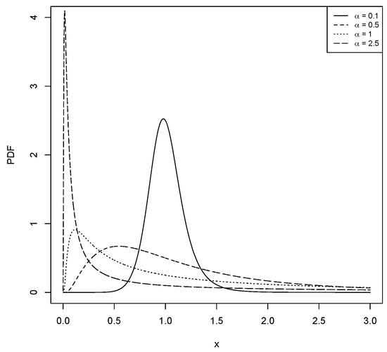
Figure 1.
The PDF for the LBS distribution with different values for and .
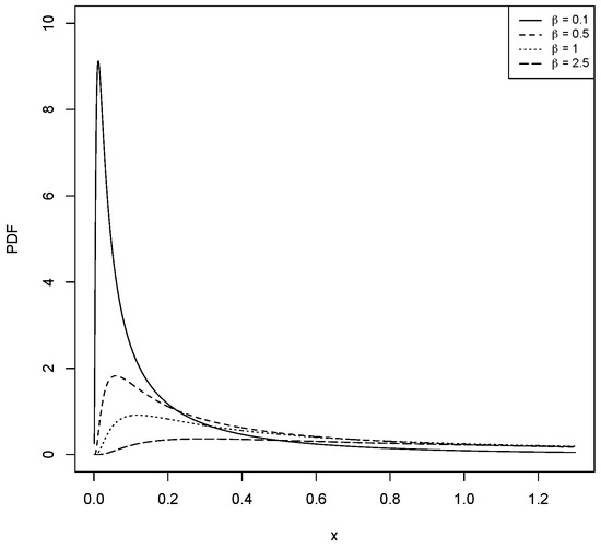
Figure 2.
The PDF for the LBS distribution with different values for and .
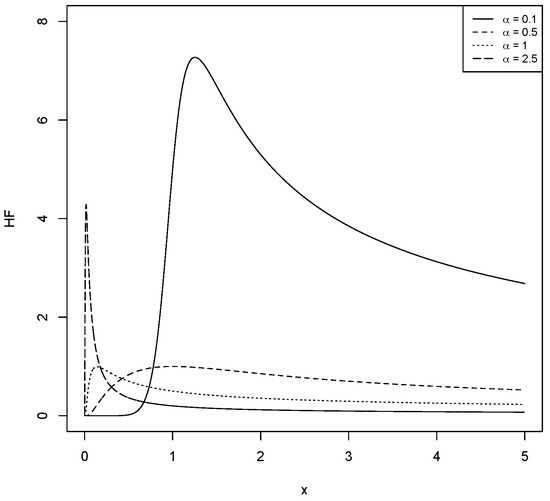
Figure 3.
The HF for the LBS distribution with different values for and .
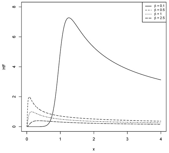
Figure 4.
The HF for the LBS distribution with different values for and .
Evidently, if the quantile function is then as follows:
Clearly, using the inverse probability integral transform on the CDF (2), Equation (4) can be used to construct random variables having as its distribution, where is the inverse of the CDF of the standard logistic distribution. Accordingly, the median will be equal to .
The HF in (5) is unimodal when and decreases when .
Lemma 1.
To study the shape of HF, let us consider the following:
a. The HF is decreasing for all values of x as .
b. If , then the HF is an upside down function with critical point; say , such that when . For the proof of Lemma 1, see [15].
In the reliability analysis, the reliability (survival) function and the mean residual life (MRL) are significant characteristics of a lifetime model. On this basis and using the CDF we can obtain the reliability (survival) function as shown below:
and
respectively, where is the considered distribution’s HF; see [16,17] in this regard. Hence, it can readily conclude from the MRL expression that it has an opposite attitude to the HF.
2.2. Order Statistics
Order statistics are another significant concept in the field of reliability analysis. Therefore, the rth order statistic’s PDF can be computed as follows: Let denote an n-sized random sample having the LBS distribution and indicate the rth order statistic. Ref. [18] define the density of the order statistic, , as:
where refers to the beta function. The of the LBS distribution is produced by substituting Equations (2) and (3) into Equation (8).
2.3. Statistical Properties
Property 1.
If T follows standard logistic distribution, i.e., , then:
Property 1 was used to calculate the LBS distribution’s expected value, variance, skewness, and kurtosis.
Property 2.
If , then
1. ;
2. ;
3. .
Property 3.
If , then, we can show that and . We also can easily obtain and by using Property 2.
3. Inference for the LBS Distribution
This section examines the inference for the LBS distribution using two methods: MLE and MME.
3.1. Maximum Likelihood Estimation
The MLEs for LBS distribution parameters are discussed in this section. Let denote an n-sized random sample having the LBS distribution with unknown parameter vector . Then, for , the log-likelihood function was constructed as follows:
The MLEs of are found by solving the nonlinear systems of equations shown below:
The second derivatives of ℓ can be calculated in the following way:
The observed information matrix is then calculated as follows:
Then, we can approximate the observed variance-covariance matrix as:
Accordingly, and asymptotic joint distribution is approximately bivariate normal, as shown by:
3.2. Modified Moment Estimation
The MMEs were proposed by [19] for BS distribution. Inspired by their research, the MMEs for LBS are proposed here by equalizing and with the relevant sample moments. In this process, the MMEs for and , represented by and , are procured as follows:
where and
The strong law of large numbers states that s and r, respectively, converge to and . The asymptotic joint distribution of and can be determined using CLT as shown below:
where
By using Taylor’s expansion, we get:
We can now calculate the asymptotic joint distribution of by utilizing the asymptotic joint distribution of .
4. Simulation Study
As previously mentioned, it is necessary to assess the estimators’ performance when the data are contaminated. In a similar way to [11,20], we take the following scenarios into consideration:
- Model 1: A model without any contamination.
- Model 2: A model with 10% of upper contamination.
- Model 3: A model with 10% of lower contamination.
- Model 4: A model with 20% of two-tailed contamination.
Therefore, this section presents the findings of the MC simulations study based on M = 10,000 simulation runs with various combinations of shape parameter and sample size values. By multiplying the upper or lower order statistics by 5 or 1/5, data contamination was achieved. In addition, the simulation study uses , , and for each scenario, with no loss of generality. It should be mentioned that all calculations were carried out using an R program, which is accessible from the authors upon request.
The simulated bias and root mean squared error (RMSE) are generated to assess estimation efficiency.
and
The simulation study’s results are visually presented in Figure 5, Figure 6, Figure 7 and Figure 8, and from these figures, we can note the following:
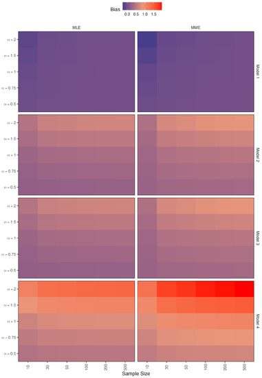
Figure 5.
Simulated biases for the estimators of .
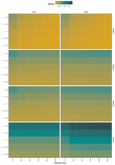
Figure 6.
Simulated RMSEs for the estimators of .
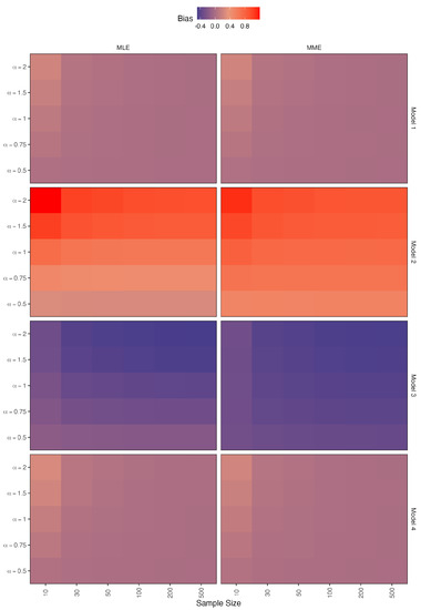
Figure 7.
Simulated biases for the estimators of .
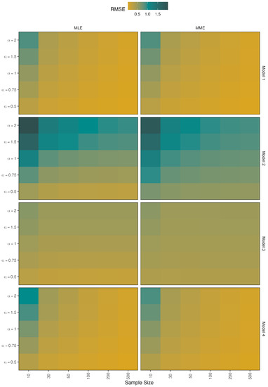
Figure 8.
Simulated RMSEs for the estimators of .
- When there is no contamination in the data, all figures show that when the sample size is increased, all methods perform well;
- The bias values of the parameter increase as the value increases in models 2 and 3;
- In the case of model 4, the bias values show that the MLE method outperforms the MME method, with MLE performing significantly better as the value decreases;
- The RMSE values of the parameter in models 2 and 3 are slightly increased when the value increases in the two methods;
- However, the RMSE values of model 4 indicate that MLE outperforms MME and that this performance improves as decreases;
- In the case of models 1 and 4, the bias values of the parameter appear to be constant around zero for both methods;
- As the value decreases in the MLE method, the bias values of models 2 and 3 approach zero;
- The RMSE values of the parameter perform similarly in the MLE and MME methods, with the values of all models getting closer to zero as the value decreases.
5. Data Analyses
We perform two data analyses in this section to compare the performance of LBS distribution with some other well-known distributions. The first set of data under examination consists of the lifetimes of 42 individuals who were diagnosed with head and neck cancer, which had previously been used by [21]. Cancer that evolves in the mouth, throat, nose, salivary glands or other parts of the head and neck is referred to as head and neck cancer. Table 1 presents the dataset:

Table 1.
Lifetimes of individuals who were diagnosed with Head and Neck Cancer.
It is important to mention that we eliminated data based on participants being lost to follow-up, as indicated by [21]; that is, we have omitted the censored data and considered the remaining ones as a complete sample. Modeling the actual data by [21] (i.e., the case of censored data) is considered for future research.
The second set of data under examination represents the lifetimes of 72 Cavia Porcellus (guinea pigs) injected with various doses of Mycobacterium tuberculosis, which was previously studied by [22] among others researchers. Mycobacterium tuberculosis is a bacterium that causes tuberculosis, a contagious disease that primarily affects the lungs. Table 2 displays the dataset:
Table 2.
Lifetimes of Cavia Porcellus injected with various doses of Mycobacterium Tuberculosis.
First, we estimate the MLEs, Bias, and RMSE of parameters, AIC and BIC of Exponential, Rayleigh, Weibull, BS, and LBS distributions, then depending on the considered dataset, we compute many explanatory data analysis (EDA) measurements, as well as their approximations based on the estimated model parameters.
Table 3 and Table 4 list the estimators of the models’ parameters as well as the AIC and BIC, while Table 5 and Table 6 present the outcomes of EDA measurements. Overall, when comparing these tables, one can observe that the estimated EDA measurements assuming the LBS distribution were very near to their observed counterparts which are calculated from the sample directly. Furthermore, the AIC and BIC indicate that the LBS distribution is a better fit. In comparison to the fitted PDFs, Figure 9 and Figure 10 show the histogram of the datasets. As can be seen in the two figures, the LBS distribution fits the data better than other distributions.
Table 3.
Values of MLEs, AIC and BIC of Exponential, Rayleigh, Weibull, BS, LBS and Laplace BS distributions for Head and Neck Cancer data.
Table 4.
Values of MLEs, AIC and BIC of Exponential, Rayleigh, Weibull, BS, LBS and Laplace BS distributions for Cavia Porcellus data.
Table 5.
EDA outcomes based on Head and Neck Cancer data.
Table 6.
EDA outcomes based on Cavia Porcellus data.
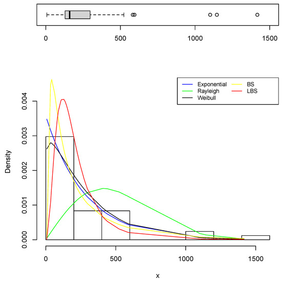
Figure 9.
The fitted PDFs based on Head and Neck Cancer data.
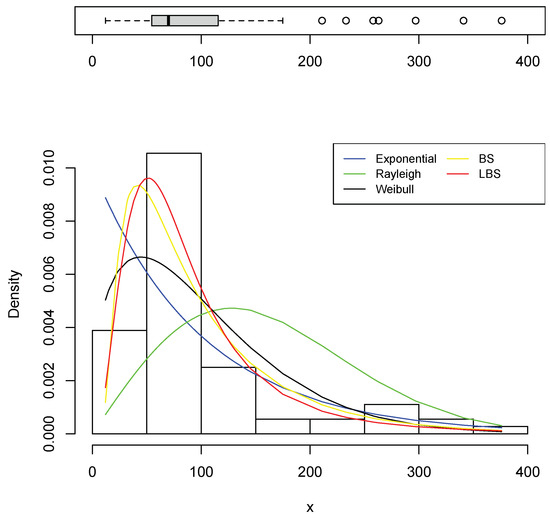
Figure 10.
The fitted PDFs based on Cavia Porcellus data.
6. Conclusions
The features of the LBS distribution and certain associated inferential methods have been discussed in this paper. The PDF of the LBS distribution might take on many shapes due to the inclusion of the shape parameter. It has either a decreasing or a unimodal HF function. When there is no contamination in the data, all approaches perform well, according to the MC simulations study. The contamination in the data may have an impact on the shape and scale parameters, with the exception of two-tailed contamination, which has no impact on the scale parameter. Finally, based on the results of the real data analysis, it is concluded that the LBS distribution, as compared to the well-known distributions, may provide a better fit to real-life data. In practice, data contamination is not the only issue researchers encounter. Another significant research challenge that needs to be addressed in future studies is data censoring, since it negatively impacts estimation efficiency and robustness. Comparing the examined estimators to Bayesian estimation in terms of performance is the last study area that one may consider.
Author Contributions
Under the idea and supervision of the corresponding author F.M.A.A., A.M.A. carried out the numerical calculations. Both F.M.A.A. and A.M.A. contributed to the final version of the manuscript. All authors have read and agreed to the published version of the manuscript.
Funding
This research received no external funding.
Institutional Review Board Statement
Not applicable.
Informed Consent Statement
Not applicable.
Data Availability Statement
Not applicable.
Acknowledgments
The authors express their sincere gratitude to the anonymous reviewers and the editors for providing useful suggestions on earlier versions of this manuscript which resulted in this improved version.
Conflicts of Interest
The authors declare no conflict of interest.
References
- Langlands, A.O.; Pocock, S.J.; Kerr, G.R.; Gore, S.M. Long-term survival of patients with breast cancer: A study of the curability of the disease. Br. Med. J. 1979, 2, 1247–1251. [Google Scholar] [CrossRef] [PubMed] [Green Version]
- Balakrishnan, N.; Kundu, D. Birnbaum–Saunders distribution: A review of models, analysis, and applications. Appl. Stoch. Model. Bus. Ind. 2019, 35, 4–49. [Google Scholar] [CrossRef] [Green Version]
- Birnbaum, Z.W.; Saunders, S.C. A new family of life distributions. J. Appl. Probab. 1969, 6, 319–327. [Google Scholar] [CrossRef]
- Birnbaum, Z.W.; Saunders, S.C. Estimation for a family of life distributions with applications to fatigue. J. Appl. Probab. 1969, 6, 328–347. [Google Scholar] [CrossRef]
- Diáz-Garciá, J.A.; Leiva-Sánchez, V. A new family of life distributions based on the elliptically contoured distributions. J. Stat. Plan. Infer. 2007, 128, 445–457, Erratum in J. Stat. Plan. Infer. 2007, 137, 1512–1513. [Google Scholar] [CrossRef]
- Leiva, V.; Riquelme, M.; Balakrishnan, N.; Sanhueza, A. Lifetime analysis based on the generalized Birnbaum–Saunders distribution. Comput. Stat. Data Anal. 2008, 52, 2079–2097. [Google Scholar] [CrossRef]
- Sanhueza, A.; Leiva, V.; Balakrishnan, N. The generalized Birnbaum–Saunders distribution and its theory, methodology, and application. Commun. Stat. Methods 2008, 37, 645–670. [Google Scholar] [CrossRef]
- Lawson, C.; Keats, J.B.; Montgomery, D.C. Comparison of robust and least-squares regression in computer-generated probability plots. IEEE Trans. Reliab. 1997, 46, 108–115. [Google Scholar] [CrossRef]
- Boudt, K.; Caliskan, D.; Croux, C. Robust explicit estimators of Weibull parameters. Metrika 2011, 73, 187–209. [Google Scholar] [CrossRef] [Green Version]
- Agostinelli, C.; Marazzi, A.; Yohai, V.J. Robust estimators of the generalized log-gamma distribution. Technometrics 2014, 56, 92–101. [Google Scholar] [CrossRef]
- Wang, M.; Park, C.; Sun, X. Simple robust parameter estimation for the Birnbaum–Saunders distribution. J. Stat. Distrib. Appl. 2015, 2, 1–11. [Google Scholar] [CrossRef] [Green Version]
- Alam, F.M.A.; Nassar, M. On Modeling Concrete Compressive Strength Data Using Laplace Birnbaum–Saunders Distribution Assuming Contaminated Information. Crystals 2021, 11, 830. [Google Scholar] [CrossRef]
- Balakrishnan, N. Handbook of the Logistic Distribution; CRC Press: Boca Raton, FL, USA, 1991. [Google Scholar]
- Xu, X.; Wang, R.; Gu, B. Statistical Analysis of Two-Parameter Generalized BS-Logistic Fatigue Life Distribution. J. Syst. Sci. Complex. 2019, 32, 1231–1250. [Google Scholar] [CrossRef]
- Alam, F.M.A.; Almalki, A.M. The hazard rate function of the logistic Birnbaum–Saunders distribution: Behavior, associated inference, and application. J. King Saud Univ.-Sci. 2021, 33, 101580. [Google Scholar] [CrossRef]
- Watson, G.; Wells, W. On the possibility of improving the mean useful life of items by eliminating those with short lives. Technometrics 1961, 3, 281–298. [Google Scholar] [CrossRef]
- Gupta, R.C.; Bradley, D.M. Representing the mean residual life in terms of the failure rate. Math. Comput. Model. 2003, 37, 1271–1280. [Google Scholar] [CrossRef] [Green Version]
- David, H.A.; Nagaraja, H.N. Order Statistics; John Wiley & Sons: Hoboken, NJ, USA, 2004. [Google Scholar]
- Ng, H.; Kundu, D.; Balakrishnan, N. Modified moment estimation for the two-parameter Birnbaum–Saunders distribution. Comput. Stat. Data Anal. 2003, 43, 283–298. [Google Scholar] [CrossRef]
- Dupuis, D.J.; Mills, J.E. Robust estimation of the Birnbaum–Saunders distribution. IEEE Trans. Reliab. 1998, 47, 88–95. [Google Scholar] [CrossRef]
- Efron, B. Logistic regression, survival analysis, and the Kaplan-Meier curve. J. Am. Stat. Assoc. 1988, 83, 414–425. [Google Scholar] [CrossRef]
- Gupta, C.R.; Kannan, N.; Raychaudhuri, A. Analysis of lognormal survival data. Math. Biosci. 1997, 139, 103–115. [Google Scholar] [CrossRef]
Publisher’s Note: MDPI stays neutral with regard to jurisdictional claims in published maps and institutional affiliations. |
© 2022 by the authors. Licensee MDPI, Basel, Switzerland. This article is an open access article distributed under the terms and conditions of the Creative Commons Attribution (CC BY) license (https://creativecommons.org/licenses/by/4.0/).