Rolling Bearing Fault Diagnosis Based on Time-Frequency Compression Fusion and Residual Time-Frequency Mixed Attention Network

Abstract

The traditional rolling bearing diagnosis algorithms have problems such as insufficient information on time-frequency images and poor feature extraction ability of the diagnosis model. These problems limit the improvement of diagnosis performance. In this article, the input of the time-frequency image and intelligent diagnosis algorithms are optimized. Firstly, the characteristics of two advanced time-frequency analysis algorithms are deeply analyzed, i.e., multisynchrosqueezing transform (MSST) and time-reassigned multisynchrosqueezing transform (TMSST). Then, we propose time-frequency compression fusion (TFCF) and a residual time-frequency mixed attention network (RTFANet). Among them, TFCF superposes and splices two time-frequency images to form dual-channel images, which can fully play the characteristics of multi-channel feature fusion of the convolutional kernel in the convolutional neural network. RTFANet assigns attention weight to the channels, time and frequency of time-frequency images, making the model pay attention to crucial time-frequency information. Meanwhile, the residual connection is introduced in the process of attention weight distribution to reduce the information loss of feature mapping. Experimental results show that the method converges after seven epochs, with a fast convergence rate and a recognition rate of 99.86%. Compared with other methods, the proposed method has better robustness and precision.

1. Introduction

Bearing is one of the essential parts of rotating machinery, and its damage causes serious failures of rotating machinery and incalculable consequences. Therefore, the bearing fault diagnosis research has become a hot spot. However, in actual working conditions, the fault signals of rotating machinery are difficult to accurately identify due to the complexity of the working condition and the influence of noise signals.

At present, A series of time-frequency analysis methods are proposed to solve these problems, for example, short-time Fourier transform (STFT) [1], continuous wavelet transform (CWT) [2], s-transform (ST) [3] and so on. The essence of time-frequency the analysis is to transform a one-dimensional time-domain signal into two-dimensional time-frequency image to reflect the variation rule of each frequency component of signal with time. Many scholars have applied it to the study of fault diagnosis. Ma et al. [4] presented a condition monitoring method based on a deep belief network (DBN) optimized by multi-order fractional Fourier transform (FRFT) and sparrow search algorithm (SSA). Firstly, they used fractional Fourier transform based on curve feature segmentation to filter fault vibration signals and extract fault characteristic frequencies. Then, the fault features are input into SSA-DBN model for training and the bearing fault features are classified, recognized and diagnosed. Zhu et al. [5] extracted the time-frequency characteristics of bearing signals through wavelet packet transform (WPT) and formed the time-frequency characteristic matrix of the signals. Secondly, multi-weight singular value decomposition (MWSVD) was constructed using singular value contribution rate and entropy weight to extract further the characteristics of the time-frequency characteristic matrix obtained by WPT. Finally, the extracted feature matrix is used as the input of the support vector machine (SVM) classifier for bearing fault diagnosis. Gituku et al. [6] used refined composite multiscale fuzzy entropy (RCMFE) for cross-domain diagnosis of bearing faults and used self-organizing fuzzy (SOF) classifier for classification. Although these methods are easy to implement, the limitations of Heisenberg’s uncertainty principle [7] prevent them from improving time and frequency resolution. To obtain time-frequency images of vibration signals with better energy concentration, Daubechies et al. [8] suggested the synchronous squeeze wavelet transform (SSWT). In essence, it is a time-frequency analysis method of energy rearrangement. Based on CWT, spectral energy is redistributed and concentrated at instantaneous frequencies [9]. Based on this idea, Huang et al. [10] proposed the synchrosqueezing S transform (SSST). Yu et al. proposed the Multisynchrosqueezing Transform (MSST) [11] and Time-reassigned Multisynchrosqueezing transform (TMSST) [12]. They performed multiple iterations based on synchronous compression transformation. They proved that the error between the time-frequency representation obtained and the ideal case becomes smaller with the increase of iterations. In other words, this method can theoretically approach the ideal time-frequency representation infinitely, which makes it widely used in the field of bearing fault diagnosis [13,14,15,16,17,18].

With the development of artificial intelligence, many scholars inducted deep learning into fault diagnosis.In bearing fault diagnosis, Major deep learning networks include autoencoder [19,20,21,22,23], Convolutional Neural Networks (CNN), generative adversarial network [24,25,26], Recurrent Neural Networks (RNN) and deep transfer learning [27,28,29].

Considering the characteristics of CNN and RNN, more and more scholars have applied them to rolling bearing fault diagnosis. The original one-dimensional vibration signal was collected as input and feature information was extracted adaptively through CNN [30,31,32,33]. However, Khorram et al. [34] combined CNN with short and long duration memory network and proposed a new convolutional short and long duration memory recurrent neural network. In addition, on that basis, some scholars generated the spectrum graph of vibration data through a time-frequency analysis and proposed a lightweight convolutional neural network to classify bearing faults [35,36]. Shenfield and Howarth [37] combined CNN and RNN. They proposed a dual-channel circulating neural network, which solved the problems of domain adaptive and high-frequency noise under actual working conditions. In addition, CNN was also used to extract the features of CWT, STFT and HHT time-frequency images, respectively [38,39,40]. These deep learning methods were novel, but they required more computing resources. Many hyperparameters need to be determined in advance, such as activation function, iteration number, learning rate, convolution kernel size, network layer number, etc.

In summary, in the intelligent fault diagnosis of rolling bearings, many scholars only used one of the methods of frequency compression and time compression. Still, they ignored the different applicable characteristics of the two kinds of methods. The compression along the frequency axis is suitable for signal components with slowly varying frequency (SCSVF). Conversely, compression along the time axis is more suitable for signal components with rapidly varying frequency (SCRVF). Rolling bearing vibration signals collected by sensors are rich and complex, often interwoven with SCSVF and SCRVF. Therefore, the combination of MSST and TMSST can be more conducive to bearing fault diagnosis. In addition, diagnostic models are divided into traditional machine learning models and deep learning models, both of which have advantages and disadvantages. The conventional method is interpreted well, but the process is complicated and has a poor-fitting ability. Deep learning automatically extracts features, but it has a high computational cost and many hyperparameters. Both methods are favored by a large number of researchers. However, the biggest obstacle to their wide application in the field of rolling bearing fault diagnosis is still how to establish a high-precision, and high-efficiency fault diagnosis model [41,42]. Therefore, it is crucial to integrate the information of multiple time-frequency images and diagnostic design models with more vital feature extraction ability and better performance. Meanwhile, the above methods have great advantages in the case of constant speed, but the advantages are not obvious in the case of variable speed. This paper proposes a fault diagnosis algorithm in the case of variable speed.

Given the above problems, this paper proposes time-frequency compression fusion (TFCF) and residual time-frequency mixed attention network (RTFANet). Firstly, two time-frequency images obtained by TMSST and MSST are fused to transform the vibration signals into dual-channel time-frequency images. Then, the attention mechanism is introduced from three aspects of channel, time, and frequency combined with the residual connection. The model can selectively focus on essential time-frequency information, avoid information overload, and extract the practical features under the framework of the convolutional neural network to solve the problem of the weak generalization ability of the model.

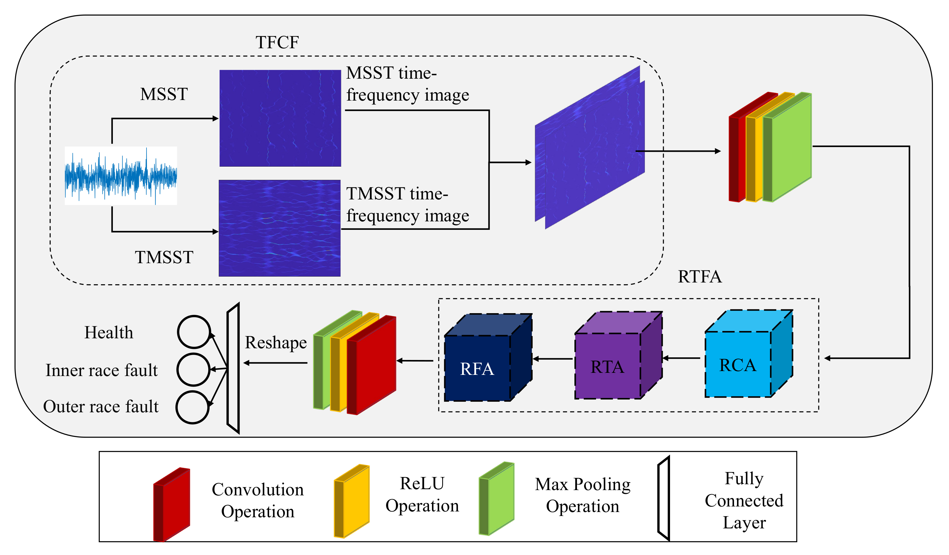
2. The Proposed Method

Figure 1 shows the overall framework of the proposed method, and the following subsections provide details of TFCF and RTFANet. As can be seen from Figure 1, the input of the RTFANet model is a TFCF dual-channel time-frequency image, and the output is the probability of this image belonging to bearing health, inner race fault and outer race fault. RTFANet first carries out the first convolution operation on the input image. After each convolution operation, the nonlinear expression ability of the model is improved by the ReLU activation function, and the parameters of the feature graph are reduced to 1/2 of the original by maximum pooling. Then, the residual time-frequency mixed attention (RTFA) is used to enhance the vital information of feature mapping. After RTFA, the second convolution operation is carried out, and the tensor dimension is reconstructed. A fully connected layer (FC) is input, and the probability of each failure is output by the softmax classifier. The details of TFCF and RTFA in Figure 1 are described in subsequent sections.

2.1. Time-Frequency Compression Fusion

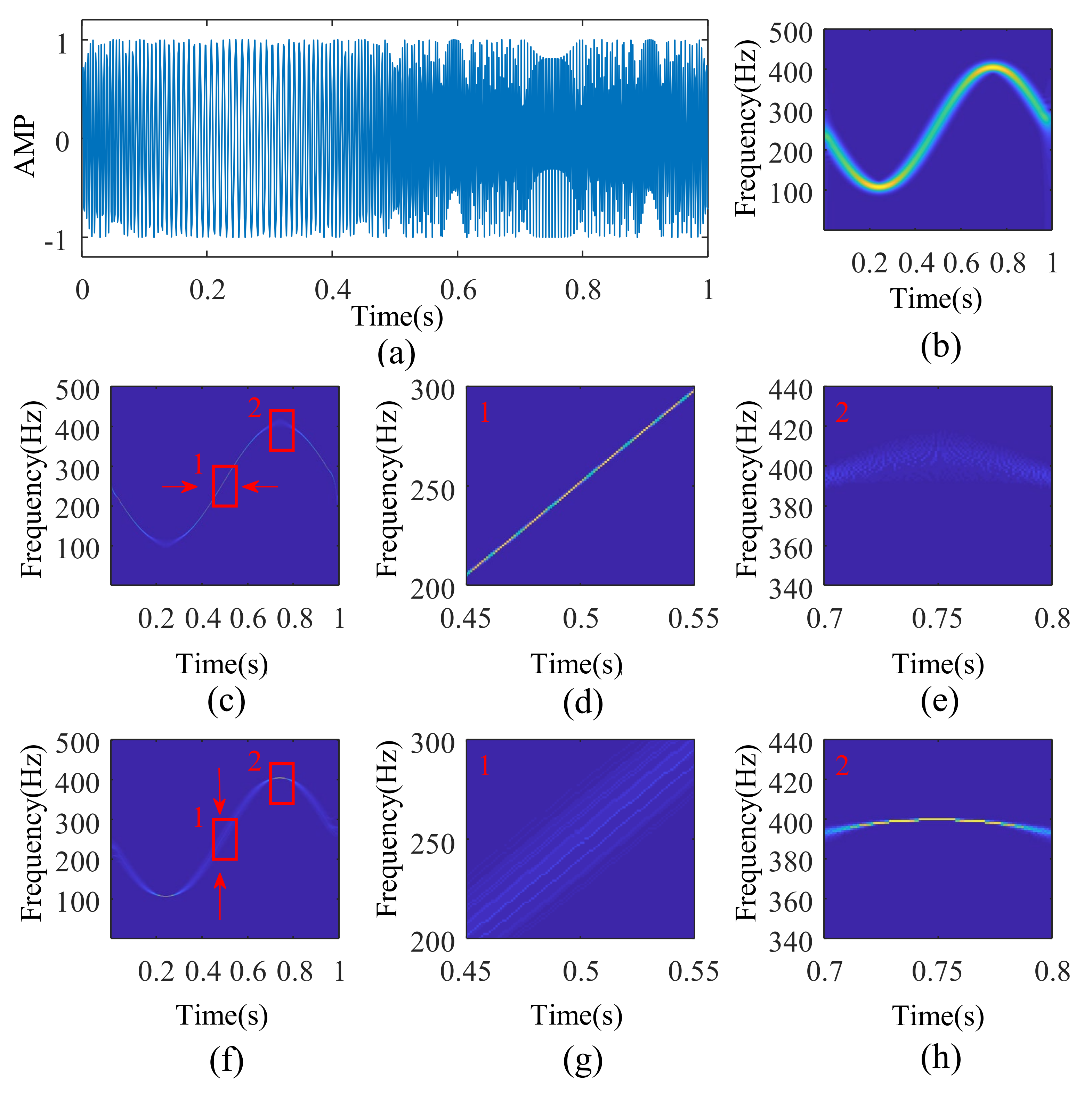
2.1.1. Time-Reassigned Multisynchrosqueezing Transform

TMSST redistributes the coefficients of time-frequency points to the time position indicated by the group delay estimation value to complete asynchronous compression transformation and obtains a new time-frequency plane, on which time redistribution operation is repeated. The group delay estimation of the signal can be expressed as:

$$\widehat{t}(\tau ,v)=j\frac{{\partial }_{v}TSTF{T}_{\delta }(\tau ,v)}{TSTF{T}_{\delta }(\tau ,v)}$$

(1)

where $\tau$ stands for time shift factor and v for frequency shift factor, when the signal does not satisfy the ideal pulse signal, there is some error between the group delay estimation and the real-time calculated by Equation (1). Fortunately, it has been shown in the literature [12] that this error can be reduced by finding a new group delay on the assumption of the original $\widehat{t}(\tau ,v)$ into $\tau$.

$$\left|\widehat{t}(\widehat{t}(\tau ,v),v)-t\right|<\left|\widehat{t}(\tau ,v)-t\right|$$

(2)

where t indicates the actual processing time of the signal, as $\widehat{t}(\widehat{t}(\tau ,v),v)$ is an iteration, this operation can be performed several times. As the number of iterations increases, the estimated group delay is closer to the actual processing time.

$$\left|{\widehat{t}}^{[N+1]}(\tau ,v)-t\right|<\left|{\widehat{t}}^{\left[N\right]}(\tau ,v)-t\right|$$

(3)

where N is a positive integer, indicating the number of iterations. ${\widehat{t}}^{\left[N\right]}(t,v)$ Indicates the group delay estimate obtained after N iterations of the time-frequency point. Specificly, ${\widehat{t}}^{\left[1\right]}(t,v)$ = $\widehat{t}(\tau ,\widehat{t}(\tau ,v))$, ${\widehat{t}}^{\left[2\right]}(t,v)$ = $\widehat{t}(\tau ,\widehat{t}(\tau ,\widehat{t}(\tau ,v)))$, ${\widehat{t}}^{\left[3\right]}(t,v)$ = $\widehat{t}(\tau ,\widehat{t}(\tau ,\widehat{t}(\tau ,\widehat{t}(\tau ,v)))$, and so on, we get ${\widehat{t}}^{\left[N\right]}(t,v)$.

After the new group delay estimation is obtained, the time-frequency coefficients of the traditional STFT can be redistributed, and the process can be expressed as:

$$TMSS{T}^{\left[N\right]}(\tau ,v)={\int }_{-\infty }^{+\infty }TSTFT(t,v)\delta (\tau -{\widehat{t}}^{\left[N\right]}(t,v))dt$$

(4)

where $TSTFT(t,v)$ is the traditional short-time Fourier transform of the model signal. $TMSS{T}^{\left[N\right]}(\tau ,v)$ is the time-frequency representation of the final time redistribution N resynchronization compression transformation. The larger N is, the more compression times and the better energy concentration of the time-frequency image.

2.1.2. Multisynchrosqueezing Transform

Unlike TMSST, MSST redistributes the coefficients of time-frequency points to the frequency position indicated by the instantaneous frequency estimation value to complete asynchronous compression transformation and obtains a new time-frequency plane. The frequency redistribution operation is repeated. The instantaneous frequency estimation of the signal can be expressed as:

$$\widehat{\omega }(\tau ,v)=\frac{\partial \tau MSTFT(\tau ,v)}{jMSTFT(\tau ,v)}$$

(5)

when the signal does not satisfy the complex sine model, there is some error between the instantaneous frequency estimate and the actual frequency calculated by Equation (5). Fortunately, literature [11] has demonstrated that this error can be reduced by obtaining a new instantaneous frequency estimate from the original $\widehat{\omega }(\tau ,v)$ into v.

$$\left|\widehat{\omega }(\tau ,\widehat{\omega }(\tau ,v))-\omega \right|<\left|\widehat{\omega }(\tau ,v)-\omega \right|$$

(6)

where $\omega$ indicates the actual frequency, and the processing of $\widehat{\omega }(\tau ,\widehat{\omega }(\tau ,v))$ can be performed multiple times. As the number of iterations increases, the instantaneous frequency is estimated to be closer to the real frequency. The iterative process is similar to TMSST.

After the new instantaneous frequency estimation is obtained, the time-frequency coefficient of the improved STFT can be redistributed. The process can be expressed as follows:

$$MSS{T}^{\left[N\right]}(\tau ,v)={\int }_{-\infty }^{+\infty }MSTFT(\tau ,\omega )\delta (v-{\widehat{\omega }}^{\left[N\right]}(\tau ,v))d\omega$$

(7)

where $MSTFT(\tau ,\omega )$ is the improved short-time Fourier transform of the model signal. $MSS{T}^{\left[N\right]}(\tau ,v)$ is the time-frequency representation of the final frequency redistribution N resynchronization compression transformation. The larger N is, the more compression times and the better energy concentration of the time-frequency image.

2.1.3. Comparison of the Two Methods

TMSST and MSST adopt different forms of short-time Fourier transform in principle from the perspective of signal reconstruction. Let the direct current component of the window function not equal to zero, that is, $G^{*}\left(0\right)\ne 0$. * is the conjugate symbol. The inverse transformation formula of TMSST can be expressed as:

$$x\left(t\right)=\frac{1}{G^{*}\left(0\right)}{\mathcal{F}}^{-1}\left\{{\int }_{-\infty }^{+\infty }TMSS{T}^{\left[N\right]}(\tau ,v)d\tau \right\}$$

(8)

where ${\mathcal{F}}^{-1}\left\{·\right\}$ represents the inverse Fourier transform operator. Assuming $g^{*}\left(0\right)\ne 0$, the inverse transformation formula of MSST can be expressed as:

$$x\left(t\right)=\frac{1}{2\pi g^{*}\left(0\right)}{\int }_{-\infty }^{+\infty }MSS{T}^{\left[N\right]}(\tau ,v)dv$$

(9)

The proof process of combined Equations (1) and (6) is as follows:

$$\begin{array}{cc}\hfill & \frac{1}{G^{*}\left(0\right)}{\mathcal{F}}^{-1}\left\{{\int }_{-\infty }^{+\infty }TMSS{T}^{\left[N\right]}(\tau ,v)d\tau \right\}\hfill \\ & =\frac{1}{2\pi G^{*}\left(0\right)}{\int }_{-\infty }^{+\infty }\left[{\int }_{-\infty }^{+\infty }TMSS{T}^{\left[N\right]}(\tau ,v)d\tau \right]e^{jvt}dv\hfill \\ \hfill & ={\mathcal{F}}^{-1}\left\{\frac{1}{G^{*}\left(0\right)}{\int }_{-\infty }^{+\infty }{\int }_{-\infty }^{+\infty }TSTFT(t,v)\delta (\tau -{\widehat{t}}^{\left[N\right]}(t,v))dtd\tau \right\}\hfill \\ \hfill & ={\mathcal{F}}^{-1}\left\{\frac{1}{G^{*}\left(0\right)}{\int }_{-\infty }^{+\infty }TSTFT(t,v)dt\right\}\hfill \\ \hfill & ={\mathcal{F}}^{-1}\left\{\frac{1}{G^{*}\left(0\right)}{\int }_{-\infty }^{+\infty }TSTFT(\tau ,v)dt\right\}\hfill \\ \hfill & ={\mathcal{F}}^{-1}\left\{\frac{1}{G^{*}\left(0\right)}{\int }_{-\infty }^{+\infty }{\int }_{-\infty }^{+\infty }x\left(t\right)g^{*}(t-\tau )e^{-jvt}dtd\tau \right\}\hfill \\ \hfill & ={\mathcal{F}}^{-1}\left\{\frac{1}{G^{*}\left(0\right)}{\int }_{-\infty }^{+\infty }x\left(t\right)\left[{\int }_{-\infty }^{+\infty }{g}^{*}(t-\tau )d\tau \right]e^{-jvt}dt\right\}\hfill \\ \hfill & ={\mathcal{F}}^{-1}\left\{\frac{1}{G^{*}\left(0\right)}{\int }_{-\infty }^{+\infty }x\left(t\right){\left[{\int }_{-\infty }^{+\infty }g\left(\tau \right)e^{-j0\tau }d\tau \right]}^{*}{e}^{-jvt}dt\right\}\hfill \\ \hfill & ={\mathcal{F}}^{-1}\left\{\frac{1}{G^{*}\left(0\right)}{\int }_{-\infty }^{+\infty }x\left(t\right)G^{*}\left(0\right)e^{-jvt}dt\right\}\hfill \\ \hfill & ={\mathcal{F}}^{-1}\left\{{\int }_{-\infty }^{+\infty }x\left(t\right)e^{-jvt}dt\right\}\hfill \\ \hfill & ={\mathcal{F}}^{-1}\left\{\mathcal{F}x\left(t\right)\right\}\hfill \\ \hfill & =x\left(t\right)\hfill \end{array}$$

(10)

The proof process of combined Equations (3) and (6) is as follows:

$$\begin{array}{cc}\hfill & \frac{1}{2\pi g^{*}\left(0\right)}{\int }_{-\infty }^{+\infty }MSS{T}^{\left[N\right]}(\tau ,v)dv\hfill \\ \hfill & =\frac{1}{2\pi g^{*}\left(0\right)}{\int }_{-\infty }^{+\infty }{\int }_{-\infty }^{+\infty }MSTFT(\tau ,\omega )\delta (v-{\widehat{\omega }}^{\left[N\right]}(\tau ,\omega ))d\omega dv\hfill \\ \hfill & =\frac{1}{2\pi g^{*}\left(0\right)}{\int }_{-\infty }^{+\infty }MSTFT(\tau ,\omega )\left[{\int }_{-\infty }^{+\infty }\delta (v-{\widehat{\omega }}^{\left[N\right]}(\tau ,\omega ))dv\right]d\omega \hfill \\ \hfill & =\frac{1}{2\pi g^{*}\left(0\right)}{\int }_{-\infty }^{+\infty }MSTFT(\tau ,v)dv\hfill \\ \hfill & =\frac{1}{2\pi g^{*}\left(0\right)}{\int }_{-\infty }^{+\infty }{\int }_{-\infty }^{+\infty }x\left(t\right)g^{*}(t-\tau )e^{-jv(t-\tau )}dtdv\hfill \\ \hfill & =\frac{1}{g^{*}\left(0\right)}{\int }_{-\infty }^{+\infty }x\left(t\right)g^{*}(t-\tau )\left[\frac{1}{2\pi }{\int }_{-\infty }^{+\infty }{e}^{-jv(t-\tau )}dv\right]dt\hfill \\ \hfill & =\frac{1}{g^{*}\left(0\right)}{\int }_{-\infty }^{+\infty }x\left(t\right)g^{*}(t-\tau )\delta (t-\tau )dt\hfill \\ \hfill & =\frac{1}{g^{*}\left(0\right)}x\left(t\right)g^{*}\left(0\right)\hfill \\ \hfill & =x\left(t\right)\hfill \end{array}$$

(11)

From the derivation of Equations (7) and (8), it can be known that whether the reassignment transform can be reconstructed depends on the short-time Fourier transform it selects. The reconstruction of the traditional STFT is completed by integrating along the time axis. Before reconstruction, the redistribution of the time-frequency coefficients along the time axis does not affect the final reconstruction result, and the traditional STFT is suitable for TMSST. The reconstruction of the improved STFT is completed by integrating it along the frequency axis. Before reconstruction, the redistribution of time-frequency coefficients along the frequency axis does not affect the final reconstruction result, and the improved STFT applies to MSST. The reconstruction properties of TMSST and MSST determine their redistribution mode to redistribute the time-frequency point coefficients of the time-frequency image to the group delay estimation and instantaneous frequency estimation of the signal, respectively. The more iterations are, the closer the group delay estimation and instantaneous frequency estimation are to the time-frequency ridgeline. However, in the time-frequency image, the time-frequency ridge line forms of different signals are different. The time-frequency ridge of the SCSVF is more inclined to the horizontal state, while that of SCRVF is vice versa.

To further investigate the applicable scenarios of TMSST and MSST, We define a simulation signal including fast and slow variable signals. The simulation signal $x_e\left(t\right)$ is defined as follows:

$$x_e\left(t\right)=cos\left\{2\pi \left[250t+\frac{150}{2\pi }cos\left(2\pi t\right)\right]\right\}$$

(12)

Figure 2 shows the time-domain waveform and related time-frequency images of the simulation signal. Figure 2a,b are the time-domain waveform and short-time Fourier transform time-frequency image of the simulation signal. It can be seen that, compared with the time-domain waveform, the time-frequency image can clearly describe the change rule of signal frequency over time to better express the characteristics of the signal. Figure 2c,f are TMSST and MSST time-frequency images of simulation signals, respectively. 1 and 2 represent the two red square box regions marked in the figure. It can be observed that the frequency changes slowly in region 1, while the frequency changes quickly in region 2, where the small red arrow represents the compression direction. Time redistribution is to move the time-frequency coefficient in Figure 2b to a new position along the time axis according to the group delay estimation calculated at the time-frequency point to realize the conversion from Figure 2b to c. Frequency redistribution refers to moving the time-frequency coefficient along the frequency axis according to instantaneous frequency estimation, as shown in Figure 2f. By comparing Figure 2c,f, it can be seen that time redistribution has a good compression effect in region 2 but leads to time-frequency energy dispersion in region 1. Frequency redistribution is the opposite. Although the two methods have the defect of energy dispersion, their advantages and disadvantages are complementary, so we can consider combining the two methods for signal analysis.

2.1.4. Time-Frequency Compression Fusion

The two STFT reconstruction methods determine the applicable redistribution methods according to the above analysis. The traditional STFT is reconstructed by integrating along the time axis, showing that it is suitable for multiple synchronous compression transform time redistribution. The improved short-time Fourier transform reconstruction method integrates along the frequency axis, which is suitable for frequency redistribution multiple synchronous compression transform. At the same time, different redistribution methods apply to other signal components. Time redistribution compresses horizontally on a time-frequency image and applies to SCRVF. Frequency redistribution compresses vertically on a time-frequency image and is more suitable for SCSVF. The two methods can learn from each other and enhance their application value.

Therefore, we propose a time-frequency compression fusion method to fuse the information of two time-frequency images obtained by TMSST and MSST, respectively. Since the scale range of the time-frequency coefficients of the two time-frequency images is not consistent, the time-frequency coefficients are normalized before fusion.

$$TF{I}^{{}^{\prime }}(t,f)=\frac{TFI(t,f)-TF{I}_{min}}{TF{I}_{max}-TF{I}_{min}}$$

(13)

where $f=\omega /2\pi$, $TF{I}_{min}$ and $TF{I}_{max}$ are the minimum and maximum values of all time-frequency coefficients in the time-frequency image, respectively, and $TF{I}^{{}^{\prime }}(t,f)$ is the result after normalization. The fusion method is named time-frequency compression fusion (TFCF). TFCF superposes and splices two time-frequency images to form dual-channel images, which can fully play the characteristics of multi-channel feature fusion of the convolutional kernel in the convolutional neural network. It is suitable for deep learning diagnosis methods.

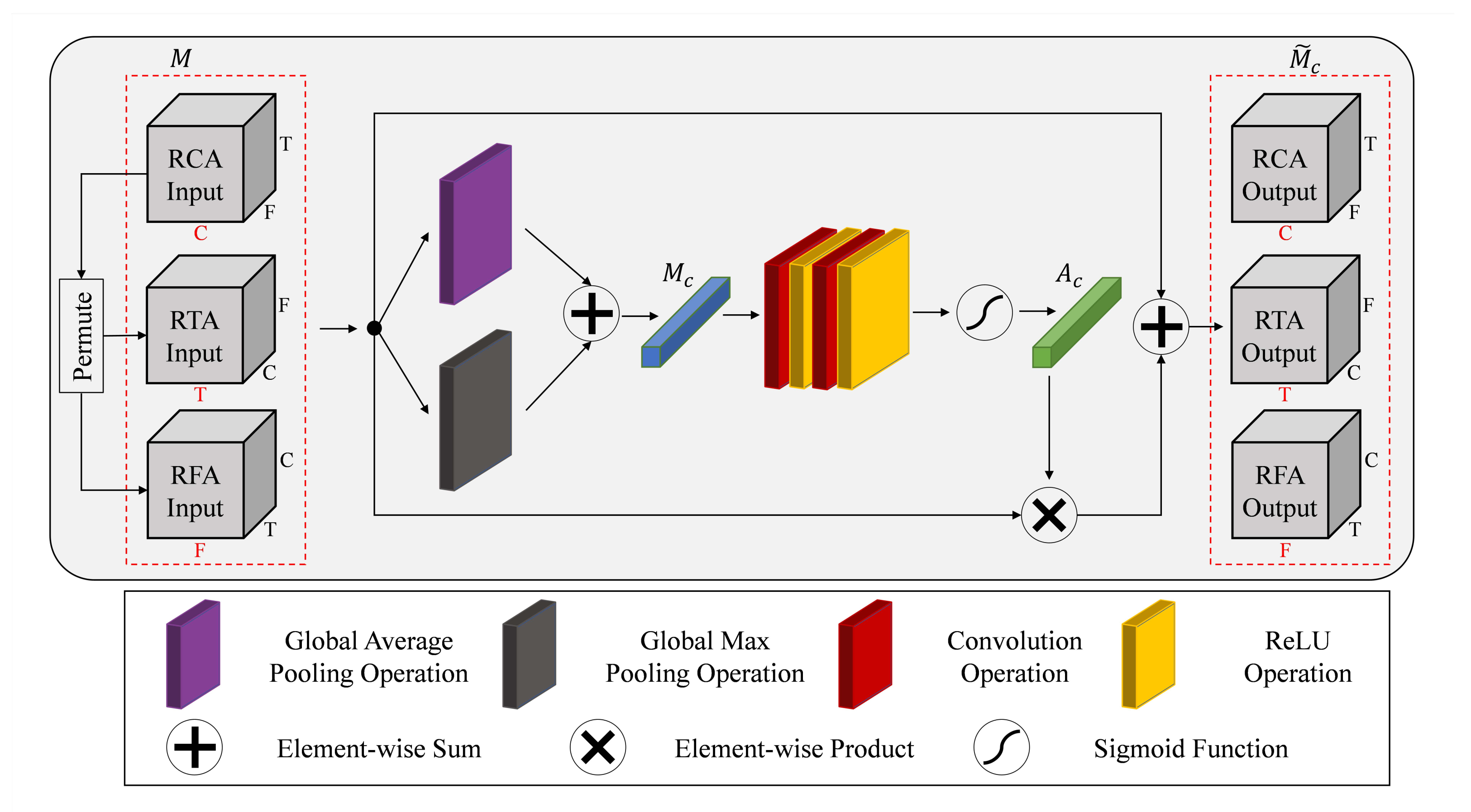
2.2. Residual Time-Frequency Mixed Attention Module Network

The convolutional neural network has shown excellent performance in image feature extraction. However, as the complexity of the network model increases, the phenomenon of gradient explosion or disappearance is easy to occurs, and the model performance is affected. Residual network structure [43] is widely used in various network models due to its special jump connection mode that can effectively alleviate gradient explosion or disappearance. The deep convolutional neural network has many parameters and performs image classification tasks well under the condition of sufficient sample size, whereas, in practical engineering, the insufficient sample size is a common problem. The sample size of vibration signals of variable speed rolling bearings used in this article is small, with only 1200 for each health condition. It is easy to overfit when directly input into the network for learning, resulting in a poor sample effect of the test set. Moreover, in the classification task, only a few important contents in the image contribute to the recognition result. Other redundant information quickly interferes with network learning and reduces network performance. Therefore, the RTFANet model is proposed. The residual time-frequency mixed attention module (RTFA) is designed and embedded into the convolutional neural network to fully extract important time-frequency features and improve the model’s classification accuracy.

2.2.1. Residual Time-Frequency Mixed Attention Module

The attention mechanism was first proposed by Bahdanau et al. [44] based on the observation rules of the visual system. In essence, it is a mechanism for allocating resources to the object of attention, that is, allocating resources according to the importance of the object. The critical parts need to be allocated more than the other parts. In deep learning, the resources allocated by the attention mechanism are reflected in weight. The information related to the recognition task is weighted more heavily, while the irrelevant information is weighted less [45].

Introducing the attention mechanism into the convolutional neural network can make the network model pay more attention to the region of interest in the input information. It makes the model ignore irrelevant features and focus only on the essential features to be extracted. The residual time-frequency mixed attention module proposed in this paper includes the channel, time and frequency. As can be seen from Figure 1, RCA, RTA and RFA are the three components of the residual time-frequency mixed attention module, and this module is stacked with the three components in sequence. When an input feature map is given, RCA pays attention to the time-frequency images of different channels. Then, RTA and RFA pay attention to SCRVF and SCSVF, respectively, and ignore the unimportant interference information. The residual time-frequency mixed attention module does not increase the model’s depth but expands the model’s width, which further improves the performance of the network model. The details of the RCA, RTA, and RFA components are shown in Figure 3.

To improve the recognition performance of a convolutional neural network for TFCF dual-channel time-frequency image feature mapping, RCA, RTA and RFA are proposed to focus on the valuable information in feature mapping. Firstly, three dimensions of input feature mapping M are defined as C, T and F, corresponding to time-frequency image channel, time and frequency, respectively. As you can see from Figure 3, RCA, RFA, and RTA differ only in input and output. RCA does not change the dimension of the input feature map, while RFA and RTA perform generalized transpose of the input feature map to realize the attention mechanism of C, T and F. Take RCA as an example, and the input characteristic map is $M\in R^{T\times F\times C}$. Then, global average pooling and maximum global pooling are performed on M, and the sum of the two results by element fuses the entire time-frequency plane information into a channel identifier $M_c\in R^{1\times 1\times C}$. Then, to further extract the effective information of $M_c$, this paper uses two convolution operations to process it and adds the ReLU function after each convolution operation to improve the nonlinear expression ability of the attention module. The first convolution layer is mainly used for dimensionality reduction, setting the dimensionality reduction ratio $r=2$. The second convolution layer is used to restore the dimensions. Finally, the element value of channel identifier $M_c$ is controlled between 0 and 1 by sigmoid function, and the channel weight information $A_c\in R^{1\times 1\times C}$ is obtained. The channel attention feature matrix $U_c\in R^{T\times F\times C}$ is obtained by weighting the input feature map M with $A_c$. The above process can be expressed as:

$$U_c=\left[\sigma \left(W_{2}R\left(W_1{M}_c\right)\right)\right]\times M$$

(14)

where $R(·)$ represents the ReLU function, $W_1\in R^{\frac{c}{r}\times C}$ and $W_2\in R^{C\times \frac{c}{r}}$ represent the weights of the two convolution operations respectively, and $\sigma (·)$ represents the Sigmoid activation function. Finally, to reduce the information loss of the channel attention feature matrix after channel weighting, the residual structure is used to fuse the channel attention feature matrix and input feature map to obtain the final channel attention feature map ${\tilde{U}}_c\in R^{T\times F\times C}$.

$${\tilde{U}}_c=U_c+M$$

(15)

The other components, RTA and RFA, differ from RCA only in the dimension positions of input features and output features after generalized transpose of input feature mapping, but the computing process is consistent.

2.2.2. Loss Function

Compared to other loss functions, cross entropy loss can avoid gradient dispersion in gradient descent calculation, leading to the decrease of learning rate. So the cross entropy loss function is a common objective function that can be divided into binary and multi-classification cross-entropy loss functions. The proposed network model realizes a multi-classification fault diagnosis based on TFCF time-frequency images of rolling bearing vibration signals. Therefore, the multi-classification cross-entropy loss function is adopted, and its expression is as follows:

$$Loss=\sum _{i=1}^N{y}_{i}log{\widehat{y}}_i$$

(16)

where N indicates the number of types of rolling bearing faults, $y_i$ indicates the actual label value of category i, and ${\widehat{y}}_i$ indicates the predicted value of category i.

3. Experiments and Results

Firstly, the collected experimental data are sampled and sorted out, and three types of fault signal are selected for time-frequency analysis. Time-frequency images are input into the proposed neural network, and then ablation experiments and comparative analysis are carried out. Finally, to verify the robustness of the proposed algorithm, tests are carried out under different sample sizes, sampling frequencies and sampling time.

3.1. The Experimental Data

The data set used from the bearing dataset of the University of Ottawa [46]. The sampling frequency of the test bench is 200 kHz. The encoder and acceleration sensor measures the speed and bearing vibration signals. The measured data include normal, inner race fault, and outer race fault. There are four speed shifting schemes, which are acceleration $(\uparrow )$, deceleration $(\downarrow )$, acceleration then deceleration $(\uparrow \downarrow )$ and deceleration then acceleration $(\downarrow \uparrow )$. The minimum speed in data collection is 9.9 Hz, and the original signal is segmented with 20,000 sampling points to ensure that each sample contains as much as possible a period. The length of each sample is also reduced to 800 to obtain a total of 3600 samples, including 1200 for each condition, which is randomly divided into the training set, validation set, and test set in the same ratio (6:2:2). More detailed information is shown in

Table 1. Bearing dataset of the University of Ottawa.

Bearing Condition	Variable Speed Condition	Training Set	Validation Set	Test Set	Class (Label)
Healthy state	$\uparrow /\downarrow /\uparrow \downarrow /\downarrow \uparrow$	720	240	240	1
Inner race fault	$\uparrow /\downarrow /\uparrow \downarrow /\downarrow \uparrow$	720	240	240	2
Outer race fault	$\uparrow /\downarrow /\uparrow \downarrow /\downarrow \uparrow$	720	240	240	3

.

To verify the superiority of our proposed method, the proportion of samples between the training set and the test set is still 3:1, in which the test set samples are the same in each experiment, and the training set is randomly selected from the rest of samples in proportion. In other words, the total sample size is 3600, the sample size of the test set is fixed at 720, 240 for each fault, and 2160 samples are randomly and evenly selected from the remaining 2880 samples in each experiment training set. The time-domain waveform of some samples is shown in Figure 4a–c. It can be seen that the time-domain waveform of vibration signals of rolling bearing with variable speed is complex, and different fault types contain signal components with frequency transients, making it difficult to extract features directly.

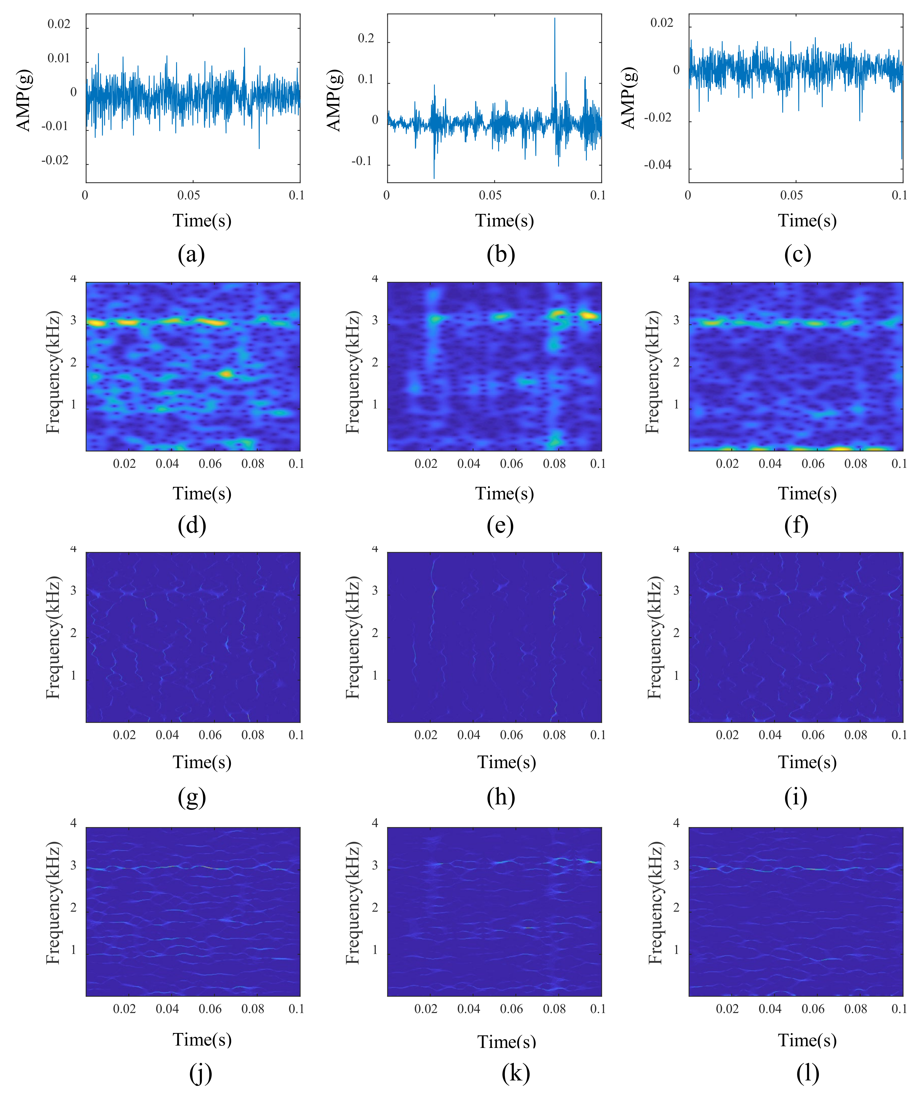
3.2. Time-Frequency Image of Vibration Signal

To improve the model’s peformance, TFCF is used to transform vibration signals into dual-channel time-frequency images containing both SCRVF and SCSVF. A sample is randomly selected from each fault type, and their STFT, TMSST and MSST time-frequency images are shown in Figure 4. It can be seen that a two-dimensional time-frequency image converted from a one-dimensional vibration signal by a time-frequency analysis algorithm can more intuitively reflect the variation rule of various frequency components in vibration signal with time.

3.3. Model Parameter Setting

In the experiment of TFCF time-frequency image classification of rolling bearing vibration signal, the setting of hyperparameters required by the training network model is as follows. The model is trained through stochastic gradient descent in small batches, and the sample size of small batches is set to 8. Adam algorithm is used to optimize the gradient value of each weight update, and the initial learning rate is set to 0.001. At the same time, L2 regularization is introduced to impose penalty constraints on weight parameters, and the penalty factor is set to 0.0001. The equal interval attenuation strategy is adopted to adjust the learning rate in the training process. The adjustment interval is set as five epochs, the adjustment multiplier gamma is set as 0.5, and other parameters can be seen in

Table 2. RTFANet model parameter settings.

The Network Layer	Nuclear Size	Step Length	Output Channel	Output Size
Input	-	-	-	$2\times 400\times 800$
Conv1	$5\times 5$	1	6	$6\times 396\times 796$
ReLU	-	-	-	$6\times 396\times 796$
Max Pooling	$2\times 2$	2	-	$6\times 198\times 398$
RCA	-	-	3; 6	$6\times 198\times 398$
RTA	-	-	99; 198	$6\times 198\times 398$
RFA	-	-	199; 398	$6\times 198\times 398$
Conv2	$5\times 5$	1	16	$16\times 194\times 394$
ReLU	-	-	-	$16\times 194\times 394$
Max Pooling	$2\times 2$	2	-	$16\times 97\times 197$
FC1	-	-	120	$1\times 1\times 120$
FC2	-	-	84	$1\times 1\times 84$
FC3	-	-	3	$1\times 1\times 3$
Softmax	-	-	3	$1\times 1\times 3$

. The kernel size of the two convolution layers in the middle of RCA, RTA, and RFA modules is $1\times 1$. The corresponding parameter settings in Table 2 refer to the number of output channels of the two convolution layers. In addition, all models are trained and tested using PyTorch deep learning framework and NVIDIA GeForce GTX 1650 GPU.

3.4. Ablation Experiments

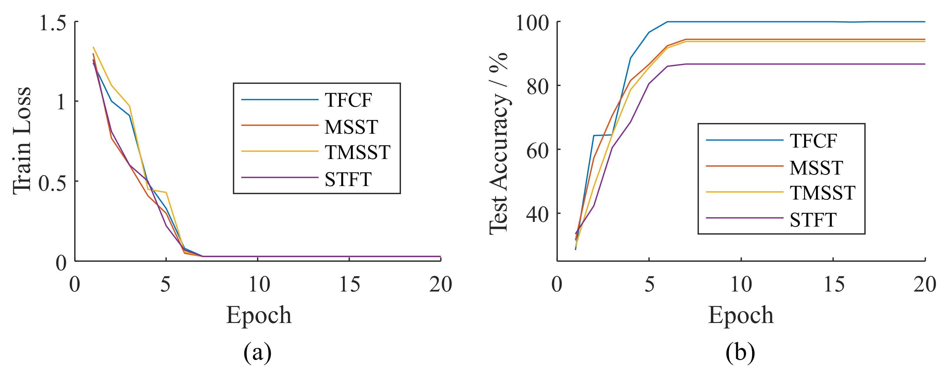
3.4.1. Different Time-Frequency Image Input

TFCF images with rich time-frequency information are proposed as the input of our diagnostic model. The time-frequency images of STFT, TMSST, MSST and TFCF are input into RTFANet for experiments to verify their superiority. Considering that the time-frequency images of STFT, TMSST and MSST are single-channel images, they are directly copied and extended into dual-channel images to ensure the consistency of model parameters. Ten experiments are conducted for each input, the training samples are randomly selected for each experiment, and the diagnostic model is input to train until convergence. During the training of optimal model obtained from ten experiments, the loss of training set and accuracy of test set varies with the number of iterations, which are shown in Figure 5. In addition, the average accuracy and standard deviation of ten experimental results are recorded in

Table 3. RTFANet recognition results of different time frequency images input.

The Time-Frequency Image	Average Recognition Accuracy (%)	Standard Deviation (%)
TFCF	99.80	0.02
MSST	94.13	0.09
TMSST	93.51	0.06
STFT	85.62	0.23

.

It can be seen from Figure 5 that no matter which time-frequency images are used as input. The model can converge to a small loss value eventually. It indicates that the model has a solid fitting ability, but the recognition accuracy of the test set is inconsistent at the end. It suggests that the information quality of images with different time-frequency is different, directly affecting the recognition results. Combined with Table 3, it can be seen that STFT has the worst effect, mainly because its time-frequency energy is too vague. MSST and TMSST compress the time-frequency energy, while the time-frequency information of some signal components is lost in compression, and the recognition effect is not good. While TFCF directly splices MSST and TMSST into a dual-channel image without eliminating any time-frequency information and achieves the highest average recognition accuracy.

To further explore the reasons for the best effect of TFCF input into RTFANet, we investigate the gradient-weighted class activation mapping of three types of TFCF images [47]. As shown in Figure 6, it can be seen that regardless of the fault type, the SCRVF, the SCSVF, and the partial dispersion time-frequency information in the TFCF image, all contribute to the final decision of the model. Therefore, it is more advantageous to use a TFCF image with more time-frequency information as the input of the network model.

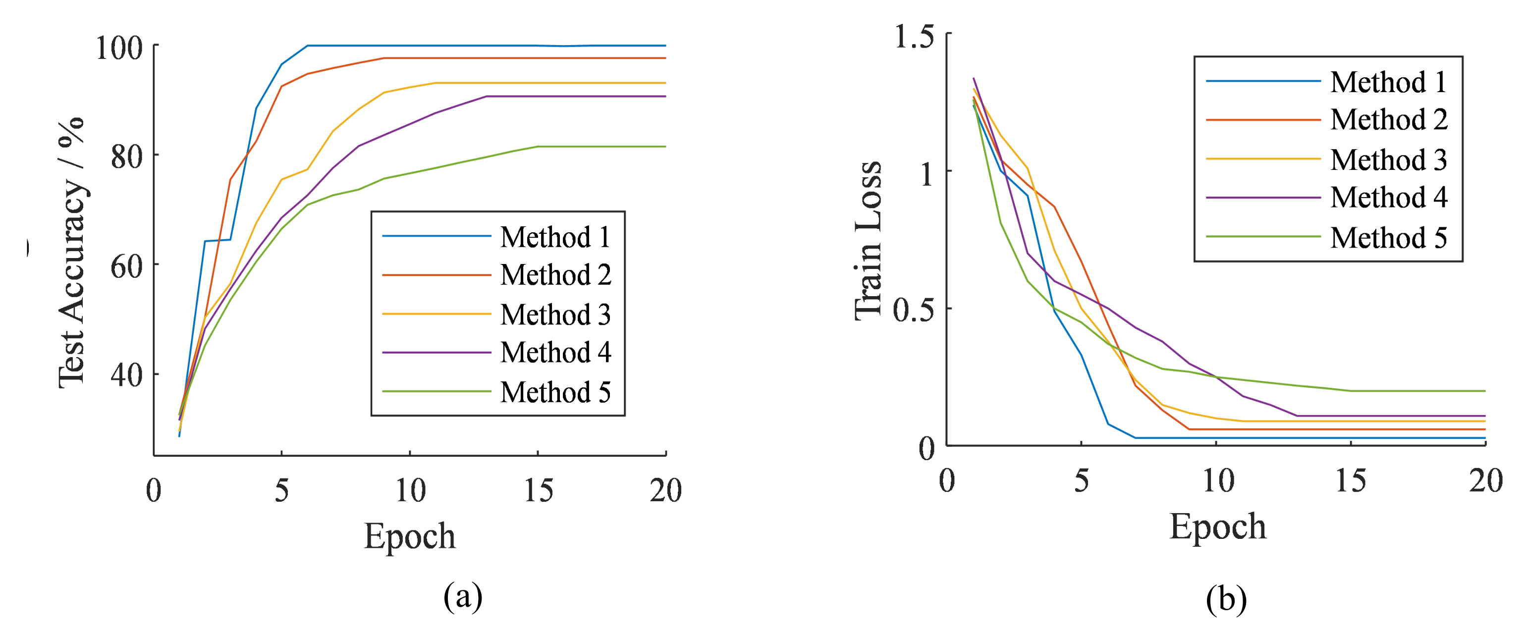
3.4.2. Different Model Combinations

To verify the effectiveness of the proposed method, different module combinations are used to identify TFCF images. The average recognition accuracy and standard deviation of ten experiments are recorded in

Table 4. Identification results of different combination models.

Number	CNN	SENet	RCA	RTA	TFA	FC	Average Accuracy	Standard Deviation
1	√	-	√	√	√	√	99.80	0.02
2	√	-	√	-	-	√	97.17	0.11
3	√	√	-	-	-	√	93.09	0.10
4	√	-	-	-	-	√	90.34	0.09
5	-	-	-	-	-	-	81.5	0.46

, and the tick mark under the module in Table 4 indicates that the module is adopted in the recognition method. The variation curves of training set loss and validation set accuracy of high accuracy models obtained by different methods in ten experiments are shown in Figure 7. It can be seen that the proposed model only converges after 7 epochs, which is faster than other methods.

Overall, the proposed method has the best recognition effect and the fastest convergence speed.

By comparing the experimental results of methods 4 and 5, it can be seen that the recognition effect is greatly improved after CNN is added to the neural network. Because the same time-frequency energy appearing in different positions of time-frequency images is essentially different, the traditional neural network directly reconstructs the tensor, completely ignoring the position information of the image. Since RCA introduces residual structure to reduce the information loss of eigenmatrix after channel weighting, it can be seen from methods 2 and 3 that RCA has a better effect than the channel attention mechanism in traditional SENet [48]. Comparing the experimental results of method 1 and method 2, it can be seen that the effect of using only the channel attention mechanism is not as good as adding an attention mechanism in all three dimensions. The main signal components of each fault type are different, and the time and frequency dimensions correspond to SCRVF and SCSVF, respectively. Time and frequency need to be further assigned to the weight of the network.

Figure 8 shows the confusion matrix of the optimal model on the test set in the ten experiments of RTFANet. It can be seen that the accuracy of the test set is 99.86%, and only one sample with an inner ring fault is incorrectly identified as the normal state. In contrast, the other samples can be correctly identified. Therefore, it can be verified that the model has good generalization ability.

3.5. Comparisons with Other Methods

To verify the superiority of the proposed algorithm,

Table 5. Comparison with other rolling bearing fault diagnosis methods.

Method	Fault Types	Accuracy (%)
TFCF+RTFANet (Proposed)	3	99.86
FRFT+SSA-DBN [4]	3	95
STFT+CNN [32]	3	96
WPT-MWSVD+SVM [5]	3	87.8
CNN-BLSTM [30]	3	99.2
ResNet-STAC-tanh [31]	3	90.77
RCMFE+SOF [6]	3	95.8

shows the recognition accuracy of different rolling bearing fault diagnosis methods. As can be seen from Table 5, the proposed method achieves the highest average accuracy of 99.86% under the same working conditions. The methods in Table 5 fail to extract the complete time-frequency information, and some even directly take the original signal as the input, which leads to information overload and increases the training time. Moreover, the model also learns irrelevant information, affecting the recognition accuracy. The proposed method introduces an attention mechanism from three perspectives of the channel, time and frequency combined with residual connection, which can obtain useful time-frequency information more effectively and facilitate subsequent model diagnosis.

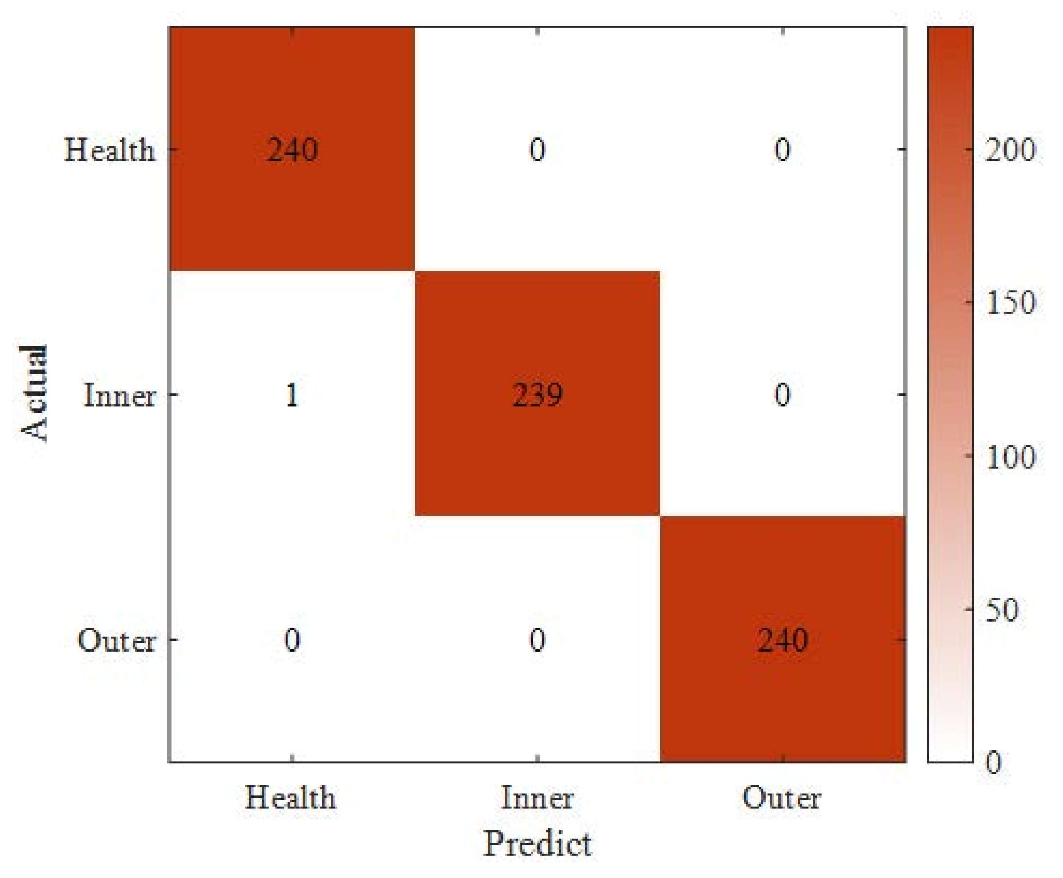
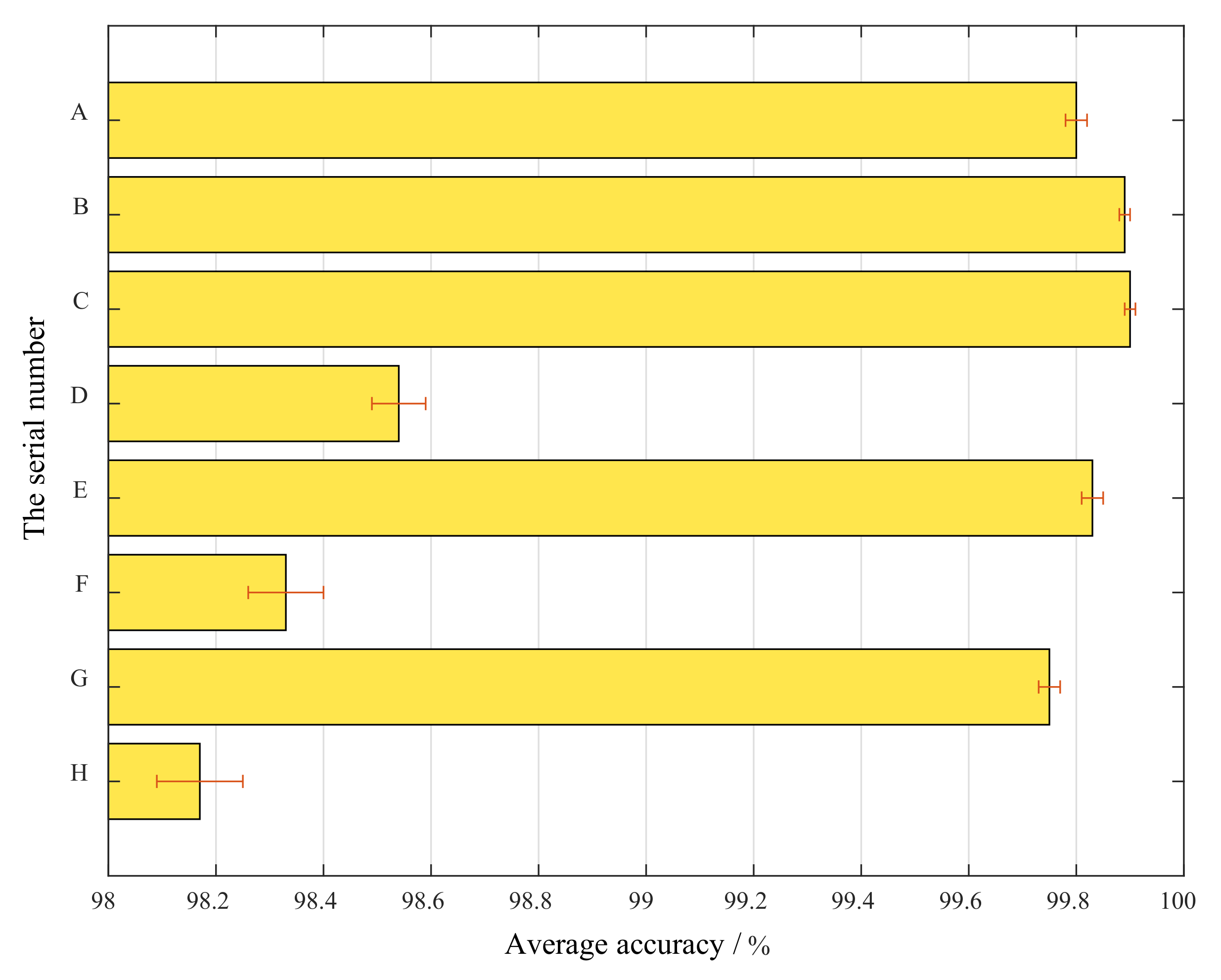
3.6. Model Performance Test

To further test the performance of the proposed method, different sample sizes, different sampling times and different sampling frequencies of each sample are investigated. The detailed experimental design is shown in

Table 6. Experimental design of model performance test.

The Serial Number	Sample Size of Training Set	Sample Size of Test Set	Sampling Time (s)	Sampling Frequency
A	2160	720	0.1	8
B	1800	1800	0.1	8
C	180	3420	0.1	8
D	108	3492	0.1	8
E	180	3420	0.05	8
F	180	3420	0.025	8
G	180	3420	0.05	4
H	180	3420	0.05	2

. Ten test experiments are conducted under each design, and the training set and test set are randomly assigned to each experiment in a fixed proportion. The experimental results are shown in Figure 9.

Combined with Table 6 and Figure 9, in general, a smaller sample size of the training set, shorter sampling time, or reduced sampling frequency affects the model performance. Still, the average accuracy is no less than 98%. Above a specific threshold condition, the average recognition accuracy of the model is more excellent than 99.70%, and experiment C is the best, with an average recognition accuracy of 99.90% and a standard deviation of only 0.01%. In addition, according to experiments A, B, C and D, when the sample size of the training set is less than 180, the accuracy decreases obviously. According to experiments C, E and F, when the sampling time is less than 0.05 s, the accuracy decreases obviously. According to experiments E, G and H, accuracy is decreased when the sampling frequency is lower than 4 kHz. In other words, there are only 60 samples in each fault type and the sampling time is only half of the rotation cycle of the lowest speed signal. And when the sampling length only includes 200 sampling points, the model can still maintain good performance.

4. Conclusions

Vibration signals of rolling bearings have the problems of overload information of time-frequency image and difficulty in fault diagnosis. To solve the problems, we propose a fault diagnosis method based on time-frequency compression fusion and residual time-frequency mixed attention network. The proposed method is verified on the bearing dataset of the University of Ottawa, and carries out the performance tests under different sample sizes, sampling times and sampling frequencies. The experimental results show that the time-frequency information of fast, slow and diffuse signals all contribute to the fault identification of the model and the TFCF time-frequency image can give full play to the performance of the diagnosis model. The residual time-frequency mixed attention module reduces the information loss after feature matrix weighting, and focuses on the important time-frequency information from the three dimensions of the TFCF image channel, time and frequency, which accelerates the convergence speed of the model training and improves the recognition accuracy to 99.86%. The proposed diagnosis model can not only solve the fault diagnosis under normal working conditions, but also maintain good performance under small sample size, short sampling time and small sampling frequency, and has broad application prospects.

References

1. Allen, J. Short term spectral analysis, synthesis, and modification by discrete Fourier transform. IEEE Trans. Acoust. Speech Signal Process. 1977, 25, 235–238. [Google Scholar] [CrossRef]
2. Morlet, J.; Arens, G.; Fourgeau, E.; Giard, D. Wave propagation and sampling theory; Part I, Complex signal and scattering in multilayered media. Geophysics 1982, 47, 203–221. [Google Scholar] [CrossRef] [Green Version]
3. Stockwell, R.; Mansinha, L.; Lowe, R. Localization of the complex spectrum: The S transform. IEEE Trans. Signal Process. 1996, 44, 998–1001. [Google Scholar] [CrossRef]
4. Ma, J.; Li, S.; Wang, X. Condition Monitoring of Rolling Bearing Based on Multi-Order FRFT and SSA-DBN. Symmetry 2022, 14, 320. [Google Scholar] [CrossRef]
5. Zhu, H.; He, Z.; Wei, J.; Wang, J.; Zhou, H. Bearing Fault Feature Extraction and Fault Diagnosis Method Based on Feature Fusion. Sensors 2021, 21, 2524. [Google Scholar] [CrossRef]
6. Gituku, E.W.; Kimotho, J.K.; Njiri, J.G. Cross-domain bearing fault diagnosis with refined composite multiscale fuzzy entropy and the self organizing fuzzy classifier. Eng. Rep. 2021, 3, e12307. [Google Scholar] [CrossRef]
7. Daubechies, I. The wavelet transform, time-frequency localization and signal analysis. IEEE Trans. Inf. Theory 1990, 36, 961–1005. [Google Scholar] [CrossRef] [Green Version]
8. Daubechies, I.; Lu, J.; Wu, H.T. Synchrosqueezed wavelet transforms: An empirical mode decomposition-like tool. Appl. Comput. Harmon. Anal. 2011, 30, 243–261. [Google Scholar] [CrossRef] [Green Version]
9. Auger, F.; Flandrin, P.; Lin, Y.T.; McLaughlin, S.; Meignen, S.; Oberlin, T.; Wu, H.T. Time-Frequency Reassignment and Synchrosqueezing: An Overview. IEEE Signal Process. Mag. 2013, 30, 32–41. [Google Scholar] [CrossRef] [Green Version]
10. Huang, Z.l.; Zhang, J.; Zhao, T.H.; Sun, Y. Synchrosqueezing S-Transform and Its Application in Seismic Spectral Decomposition. IEEE Trans. Geosci. Remote. Sens. 2015, 54, 1–9. [Google Scholar] [CrossRef]
11. Yu, G.; Wang, Z.; Zhao, P. Multisynchrosqueezing Transform. IEEE Trans. Ind. Electron. 2019, 66, 5441–5455. [Google Scholar] [CrossRef]
12. Yu, G.; Lin, T.; Wang, Z.; Li, Y. Time-Reassigned Multisynchrosqueezing Transform for Bearing Fault Diagnosis of Rotating Machinery. IEEE Trans. Ind. Electron. 2021, 68, 1486–1496. [Google Scholar] [CrossRef]
13. Sun, G.; Gao, Y.; Lin, K.; Hu, Y. Fine-Grained Fault Diagnosis Method of Rolling Bearing Combining Multisynchrosqueezing Transform and Sparse Feature Coding Based on Dictionary Learning. Shock Vib. 2019, 2019, 1531079. [Google Scholar] [CrossRef] [Green Version]
14. Sun, G.; Gao, Y.; Xu, Y.; Feng, W. Data-Driven Fault Diagnosis Method Based on Second-Order Time-Reassigned Multisynchrosqueezing Transform and Evenly Mini-Batch Training. IEEE Access 2020, 8, 120859–120869. [Google Scholar] [CrossRef]
15. Yu, G. A multisynchrosqueezing-based high-resolution time-frequency analysis tool for the analysis of non-stationary signals. J. Sound Vib. 2020, 492, 115813. [Google Scholar] [CrossRef]
16. Zheng, J.; Gu, M.; Pan, H.; Tong, J. A Fault Classification Method for Rolling Bearing Based on Multisynchrosqueezing Transform and WOA-SMM. IEEE Access 2020, 8, 215355–215364. [Google Scholar] [CrossRef]
17. Yu, K.; Wang, X.; Cheng, Y. A Post-Processing Method for Time-Reassigned Multisynchrosqueezing Transform and Its Application in Processing the Strong Frequency-Varying Signal. IEEE Trans. Instrum. Meas. 2021, 70, 1–11. [Google Scholar] [CrossRef]
18. Feiyue, D.; Liu, C.; Liu, Y.; Hao, R. A Hybrid SVD-Based Denoising and Self-Adaptive TMSST for High-Speed Train Axle Bearing Fault Detection. Sensors 2021, 21, 6025. [Google Scholar]
19. Lin, Y.; Li, Y.; Yin, X.; Dou, Z. Multisensor Fault Diagnosis Modeling Based on the Evidence Theory. IEEE Trans. Reliab. 2018, 67, 513–521. [Google Scholar] [CrossRef]
20. Mao, W.; Feng, W.; Liu, Y.; Zhang, D.; Liang, X. A new deep auto-encoder method with fusing discriminant information for bearing fault diagnosis. Mech. Syst. Signal Process. 2021, 150, 107233. [Google Scholar] [CrossRef]
21. Mao, W.; Feng, W.; Liang, X. A novel deep output kernel learning method for bearing fault structural diagnosis. Mech. Syst. Signal Process. 2019, 117, 293–318. [Google Scholar] [CrossRef]
22. Cui, M.; Wang, Y.; Lin, X.; Zhong, M. Fault Diagnosis of Rolling Bearings Based on an Improved Stack Autoencoder and Support Vector Machine. IEEE Sens. J. 2020, 21, 4927–4937. [Google Scholar] [CrossRef]
23. Zhang, S.; Ye, F.; Wang, B.; Habetler, T. Semi-Supervised Bearing Fault Diagnosis and Classification Using Variational Autoencoder-Based Deep Generative Models. IEEE Sens. J. 2020, 21, 6476–6486. [Google Scholar] [CrossRef]
24. Dixit, S.; Verma, N. Intelligent Condition-Based Monitoring of Rotary Machines With Few Samples. IEEE Sens. J. 2020, 20, 14337–14346. [Google Scholar] [CrossRef]
25. Xu, M.; Wang, Y. An Imbalanced Fault Diagnosis Method for Rolling Bearing Based on Semi-Supervised Conditional Generative Adversarial Network With Spectral Normalization. IEEE Access 2021, 9, 27736–27747. [Google Scholar] [CrossRef]
26. Zheng, T.; Song, L.; Wang, J.; Teng, W.; Xu, X.; Ma, C. Data synthesis using dual discriminator conditional generative adversarial networks for imbalanced fault diagnosis of rolling bearings. Measurements 2020, 158, 107741. [Google Scholar] [CrossRef]
27. Yin, H.; Li, Z.; Zuo, J.; Liu, H.; Yang, K.; Li, F. Wasserstein Generative Adversarial Network and Convolutional Neural Network (WG-CNN) for Bearing Fault Diagnosis. Math. Probl. Eng. 2020, 2020, 2604191. [Google Scholar] [CrossRef]
28. Wang, M.; Lin, Y.; Tian, Q.; Si, G. Transfer Learning Promotes 6G Wireless Communications: Recent Advances and Future Challenges. IEEE Trans. Reliab. 2021, 70, 790–807. [Google Scholar] [CrossRef]
29. Lin, Y.; Tu, Y.; Dou, Z. An Improved Neural Network Pruning Technology for Automatic Modulation Classification in Edge Devices. IEEE Trans. Veh. Technol. 2020, 69, 5703–5706. [Google Scholar] [CrossRef]
30. You, D.; Chen, L.; Liu, F.; Zhang, Y.; Shang, W.; Hu, Y.; Liu, W. Intelligent Fault Diagnosis of Bearing Based on Convolutional Neural Network and Bidirectional Long Short-Term Memory. Shock Vib. 2021, 2021, 7346352. [Google Scholar] [CrossRef]
31. Zhang, T.; Liu, S.; Wei, Y.; Zhang, H. A novel feature adaptive extraction method based on deep learning for bearing fault diagnosis. Measurement 2021, 185, 110030. [Google Scholar] [CrossRef]
32. Wang, Y.; Huang, S.; Dai, J.; Tang, J. A Novel Bearing Fault Diagnosis Methodology Based on SVD and One-Dimensional Convolutional Neural Network. Shock Vib. 2020, 2020, 1850286. [Google Scholar] [CrossRef]
33. Ji, M.; Peng, G.; He, J.; Liu, S.; Chen, Z.; Li, S. A Two-Stage, Intelligent Bearing-Fault-Diagnosis Method Using Order-Tracking and a One-Dimensional Convolutional Neural Network with Variable Speeds. Sensors 2021, 21, 675. [Google Scholar] [CrossRef] [PubMed]
34. Khorram, A.; Khalooei, M.; Rezghi, M. End-to-end CNN + LSTM deep learning approach for bearing fault diagnosis. Appl. Intell. 2021, 51, 1–16. [Google Scholar] [CrossRef]
35. Bera, A.; Dutta, A.; Dhara, A.K. Deep Learning based Fault Classification Algorithm for Roller Bearings using Time-Frequency Localized Features. In Proceedings of the International Conference on Computing, Communication, and Intelligent Systems (ICCCIS), Greater Noida, India, 19–20 February 2021; pp. 419–424. [Google Scholar]
36. Xu, Y.; Li, Z.; Wang, S.; Li, W.; Sarkodie-Gyan, T.; Feng, S. A hybrid deep-learning model for fault diagnosis of rolling bearings. Measurement 2021, 169, 108502. [Google Scholar] [CrossRef]
37. Shenfield, A.; Howarth, M. A Novel Deep Learning Model for the Detection and Identification of Rolling Element-Bearing Faults. Sensors 2020, 20, 5112. [Google Scholar] [CrossRef]
38. Guo, S.; Yang, T.; Gao, W.; Zhang, C. A Novel Fault Diagnosis Method for Rotating Machinery Based on a Convolutional Neural Network. Sensors 2018, 18, 1429. [Google Scholar] [CrossRef] [Green Version]
39. Duan, S.; Zheng, H.; Liu, J. A Novel Classification Method for Flutter Signals Based on the CNN and STFT. Int. J. Aerosp. Eng. 2019, 2019, 1–8. [Google Scholar] [CrossRef]
40. Guo, M.F.; Yang, N.C.; Chen, W.F. Deep-Learning-Based Fault Classification Using Hilbert-Huang Transform and Convolutional Neural Network in Power Distribution Systems. IEEE Sensors J. 2019, 19, 6905–6913. [Google Scholar] [CrossRef]
41. Shao, H.; Zhang, X.; Cheng, J.; Yu, Y. Intelligent Fault Diagnosis of Bearing Using Enhanced Deep Transfer Auto-encoders. J. Mech. Eng. 2020, 9, 84–90. [Google Scholar]
42. Zhuang, Z.; Lv, H.; Xu, J.; Zizhao, H.; Qin, W. A Deep Learning Method for Bearing Fault Diagnosis through Stacked Residual Dilated Convolutions. Appl. Sci. 2019, 9, 1823. [Google Scholar] [CrossRef] [Green Version]
43. He, K.; Zhang, X.; Ren, S.; Sun, J. Deep Residual Learning for Image Recognition. In Proceedings of the IEEE Conference on Computer Vision and Pattern Recognition (CVPR), Las Vegas, NV, USA, 27–30 June 2016; pp. 770–778. [Google Scholar]
44. Bahdanau, D.; Cho, K.; Bengio, Y. Neural Machine Translation by Jointly Learning to Align and Translate. arXiv 2014, arXiv:1409.0473. [Google Scholar]
45. Mnih, V.; Heess, N.; Graves, A.; Kavukcuoglu, K. Recurrent Models of Visual Attention. In Proceedings of the 27th International Conference on Neural Information Processing Systems, Montreal, QC, Canada, 8–13 December 2014; Volume 2, pp. 2204–2212. [Google Scholar]
46. Huang, H.; Baddour, N. Bearing vibration data collected under time-varying rotational speed conditions. Data Brief 2018, 21, 1745–1749. [Google Scholar] [CrossRef] [PubMed]
47. Selvaraju, R.R.; Cogswell, M.; Das, A.; Vedantam, R.; Parikh, D.; Batra, D. Grad-CAM: Visual Explanations from Deep Networks via Gradient-Based Localization. In Proceedings of the IEEE International Conference on Computer Vision (ICCV), Venice, Italy, 22–29 October 2017; pp. 618–626. [Google Scholar]
48. Hu, J.; Shen, L.; Albanie, S.; Sun, G.; Wu, E. Squeeze-and-Excitation Networks. IEEE Trans. Pattern Anal. Mach. Intell. 2020, 42, 2011–2023. [Google Scholar] [CrossRef] [PubMed] [Green Version]
Figure 1. Overall model architecture.
Applsci 12 04831 g001
Figure 2. Time–frequency analysis and comparison of simulation signals: (a) time–domain waveform of simulation signal x e ( t ) : (bf) are STFT, TMSST and MSST time–frequency images of simulation signals, respectively; (d,e) are enlarged images of regions 1 and 2 in (c), respectively; (g,h) are respectively enlarged images of regions 1 and 2 in (f).
Applsci 12 04831 g002
Figure 3. Structure of residual time–frequency mixed attention module.
Applsci 12 04831 g003
Figure 4. Time–frequency images of vibration signal of rolling bearing: (ac) are time–domain waveforms of normal, inner race fault and outer race fault samples respectively; (df) are STFT time-frequency images corresponding to (ac) respectively; (gi) are TMSST time-frequency images corresponding to (ac); (jl) are MSST time-frequency images corresponding to (ac) respectively.
Applsci 12 04831 g004
Figure 5. Training of RTFANet model under different inputs: (a) curve of training set loss; (b) curve of the accuracy of the test set.
Applsci 12 04831 g005
Figure 6. Gradient–weighted class activation mapping for different fault samples: (a) normal; (b) inner race fault; (c) outer race fault.
Applsci 12 04831 g006
Figure 7. Training of different combination models: (a) curve of training set loss; (b) accuracy curve of the test set.
Applsci 12 04831 g007
Figure 8. RTFANet model confusion matrix on test set.
Applsci 12 04831 g008
Figure 9. Experimental results of model performance test.
Applsci 12 04831 g009