Detecting the Speed Change Intention from EEG Signals: From the Offline and Pseudo-Online Analysis to an Online Closed-Loop Validation

Abstract

Control of assistive devices by voluntary user intention is an underdeveloped topic in the Brain–Machine Interfaces (BMI) literature. In this work, a preliminary real-time BMI for the speed control of an exoskeleton is presented. First, an offline analysis for the selection of the intention patterns based on the optimum features and electrodes is proposed. This is carried out comparing three different classification models: monotonous walk vs. increasing and decreasing change speed intentions, monotonous walk vs. only increasing intention, and monotonous walk vs. only decreasing intention. The results indicate that, among the features tested, the most suitable parameter to represent these models are the Hjorth statistics in alpha and beta frequency bands. The average offline classification accuracy for the offline cross-validation of the three models obtained is 68 ± 11%. This selection is also tested following a pseudo-online analysis, simulating a real-time detection of the subject’s intentions to change speed. The average results indices of the three models during this pseudoanalysis are of a 42% true positive ratio and a false positive rate per minute of 9. Finally, in order to check the viability of the approach with an exoskeleton, a case of study is presented. During the experimental session, the pros and cons of the implementation of a closed-loop control of speed change for the H3 exoskeleton through EEG analysis are commented.

1. Introduction

Motor disabilities due to stroke impairment or spinal cord injury are an increasing problem in our modern society [1]. In the rehabilitation field, the current conventional motor therapies consist of the execution of intensive and repetitive sessions to mobilize the affected limb. These therapies are used to facilitate the recovery and learning postural movement allowing to adapt the disability to the daily life. However, these procedures are turning the focus on increasing cognitive involvement in order to increase the activation of neural plasticity processes [2].

Cognitive involvement can be achieved in many ways, including through the recording of brain activity establishing a direct connection between the mental task and the user. There are many ways to decode user’s intention from brain activity [3]. For the detection of motor intention, the most common paradigms are: Movement-Related Cortical Potentials (MRCPs) and Event-Related (De)Synchronization (ERD/ERS), each with different latency and frequency characteristics regarding the eliciting event. MRCP are associated with low frequency changes (0.05–3 Hz) occurring as early as 0.5–2 s. ERD/ERS is described as a change of power in the alpha (8–12 Hz) and beta (13–30 Hz) bands. This event is temporally characterized up to 2 s before the self-paced movement [4]. Both are associated with movement imagination and execution.

Concerning the practically decodification of both potentials, MRCP provides timing information about movement stages and planning execution, but it is very unstable against noise and not so useful in single trial analysis [5]. On the other hand, ERD/ERS does not provide precise timing information about different stages of movement planning, preparation and execution, but ERD/ERS has been shown to be detectable from single trial EEG [6] and less variable to noise than MRCP [7].

These qualities of the ERD/ERS potential allow prediction of motor intention and could be useful for assisting the user’s movement. This connection between this decoding potential recorded in the scalp and the motor execution is called Brain–Machine Interface (BMI). The information is registered by noninvasive electroencephalography (EEG) and the interpretation of the patterns extracted from it can be used to send commands to an assistive device. This can be used to control devices such as a weelchair or an exoskeleton and help non-able bodied subjects not only from rehabilitation, but assistance perspectives. Both approaches have been studied in the literature: the rehabilitation approach is focused in the BMI neuroplasticity elicitation [8]; and the assistance, more focused on the control loop decision efficiency [9]. The ERD/ERS intention paradigm can facilitate the device adaptation in different gait scenarios. Since most of the neural changes appear before the onset of movement, the assistive movement appears more natural and eliminates undesirable delays and frustrating waits. The possibility of using BMIs for movement assistance has led to the study of EEG-encoded movement patterns. There are several studies analyzing different lower-limb motion controls, for example: start–stop, change direction, stand-up/sit-down and change speed.

The decoding of start–stop walking is analyzed in Ortiz et al. in offline and pseudo-online analysis. In the study, the data window was chosen both in an interval of −2 to 2 s after it. The Stockwell transform and the empirical mode decomposition (EMD) [10] were used to extract time-frequency features. In Sburlea et al. [11], start walking EEG was collected and analyzed in pseudo-online methology using a window from −1.5 to 0 s before the movement, performing an unbalancing class training. The temporal MRCP and spectral ERD/ERS characteristics were tested separately and in combination, with a predominance of the influence precision of the MRCP features. In Shafiul et al. [6], the temporal analysis interval was chosen between −2 s to 0 s before the movement onset, as an special subdivided windows’ feature extraction method. All Hjorth parameters were computed and a pseudo-online analysis was performed. In [12], a wavelet transform analysis was performed in the same procedural experiment. Both experiments [6,12] work with the Artifact Subspace Reconstruction (ASR) filter and a baseline correction for the pseudo-online Linear Support Vector Machine (SVM) classification. However, the former one has been reported as a huge gap to bridge in real-time applications. In [13], another gait-stop intention paradigm was performed with ASR and combining common spatial pattern (CSP) and linear discriminant analysis classification.

In [14], the change of direction is studied offline using a window prior to the change, a KNN classifier differentiates a large and varied number of features. In [15], a protocol for an exoskeleton control based on the decoding of the EEG signal is presented. It tries to differentiate between four motion classes (walk, turn-right, stop and turn-left). This is done by a pseudo-online analysis using a MRCP paradigm with ASR filtering and multiple kernel learning, reporting high accuracy rates. However, the protocol marks when the user should perform the action, not allowing a free intention of the subject. This makes the signals susceptible to possible Event Related Potentials (ERP). A similar protocol is performed at [16], with the same motor states analyzed, but the MRCP patterns are reduced with local fishers’s discriminant and classified with an unsupervised Gaussian Mixture Model (GMM).

Finally, the change of speed has also been analyzed. In [17], Lisi et al. study the correlation between the EEG and increment/decrement speed changes. In the offline analysis, the speed change window is chosen between −4 and 4 s after the change, while the constant speed window is chosen between −12 and −4 s. reported suppression in mu rhythm ranging from −1 to 3 s, nevertheless the largest magnitude of ERD/ERS is located in the mu band between 0.5 and 2 s and beta rhythm starting near the onset and ending at 2 s. The most studied approach of all these is the start and stop one. This action is very interesting for voluntary gait control. Regarding closed-loop control, the relevant investigations in the literature are:

The aforementioned research in [13] proposes a protocol to decode start/stop intentions from EEG signals based on ERD/ERS features in a pseudo-online methodology with an exoskeleton. It reports a TP of 89.0 ± 0.8% and FP/min of 13.6 ± 0.4. closed-loop real-time detection results report a TP of 92.3% and a FP/min ratio of 28.4 ± 35.2. In addition, in the work of Kilicarslan et al. [16] the closed-loop only is performed for the walk and stop patterns. Although the decoding results are close to 100%, reliable metrics are not reported.

However, the modulation of the transition between gait states, such as direction or speed changes are a less researched topic and there are not many examples in the literature. Training the model with the exoskeleton is a critical point in these paradigms. In [15,16], marks on the ground are used to instruct the subject to perform the change at a certain point. The model must be trained with data acquired with the exoskeleton, so that later it can be tested in closed-loop control efficiently and with good performance [18]. No closed-loop studies were found for these paradigms. This indicates that there is a clear gap on this approach in the literature and that further research is needed for the development of robust closed-loop models.

This work tries to close this gap developing a closed-loop experiment to detect the intention of changing speed moments before the subject has executed it. The objective is to improve the tool to a viable stage for its posterior use in non-able bodied subjects. With this in mind, several studies are performed. In the first one, a group of features is analyzed offline in a wide spectrum of frequency bands. This is used to identify the parameters that maximize the differences between the mental states in three different models: monotonous walk vs. increasing and decreasing change speed intentions, monotonous walk vs. only increasing intention, and monotonous walk vs. only decreasing intention. After this, the combination of the optimized features is analyzed by a pseudo-online approach previous to its test in real time for the closed-loop control of an H3 exoskeleton.

The paper is organized as follows. Section 2 describes the methods employed for registering the EEG, offline analysis for design of the BMI, and pseudo-online validation methodology. In addition, online closed-loop BMI protocol and operation is presented. Section 3 describes the results for both the offline and pseudo-online analysis that are used to parameterize the online closed-loop BMI of which results of the experimental study are also shown. Section 4 summarize the results of the approach and propose improvements and lines of advance. Finally, Section 5 summarizes the main conclusions of the paper.

2. Materials and Methods

This section provides detailed information about the experimental protocols, equipment and methodology for data acquisition and signal processing.

2.1. Subjects

Five healthy subjects, with an average age of 25.4 ± 3.5 years (1 female and 4 males) participated in the study. The subjects reported no diseases and they participated voluntarily in the study by giving their informed consent according to the Helsinki declaration approved by the Ethics Committee of the Responsible Research Office of Miguel Hernandez University of Elche (Spain).

2.2. Equipment

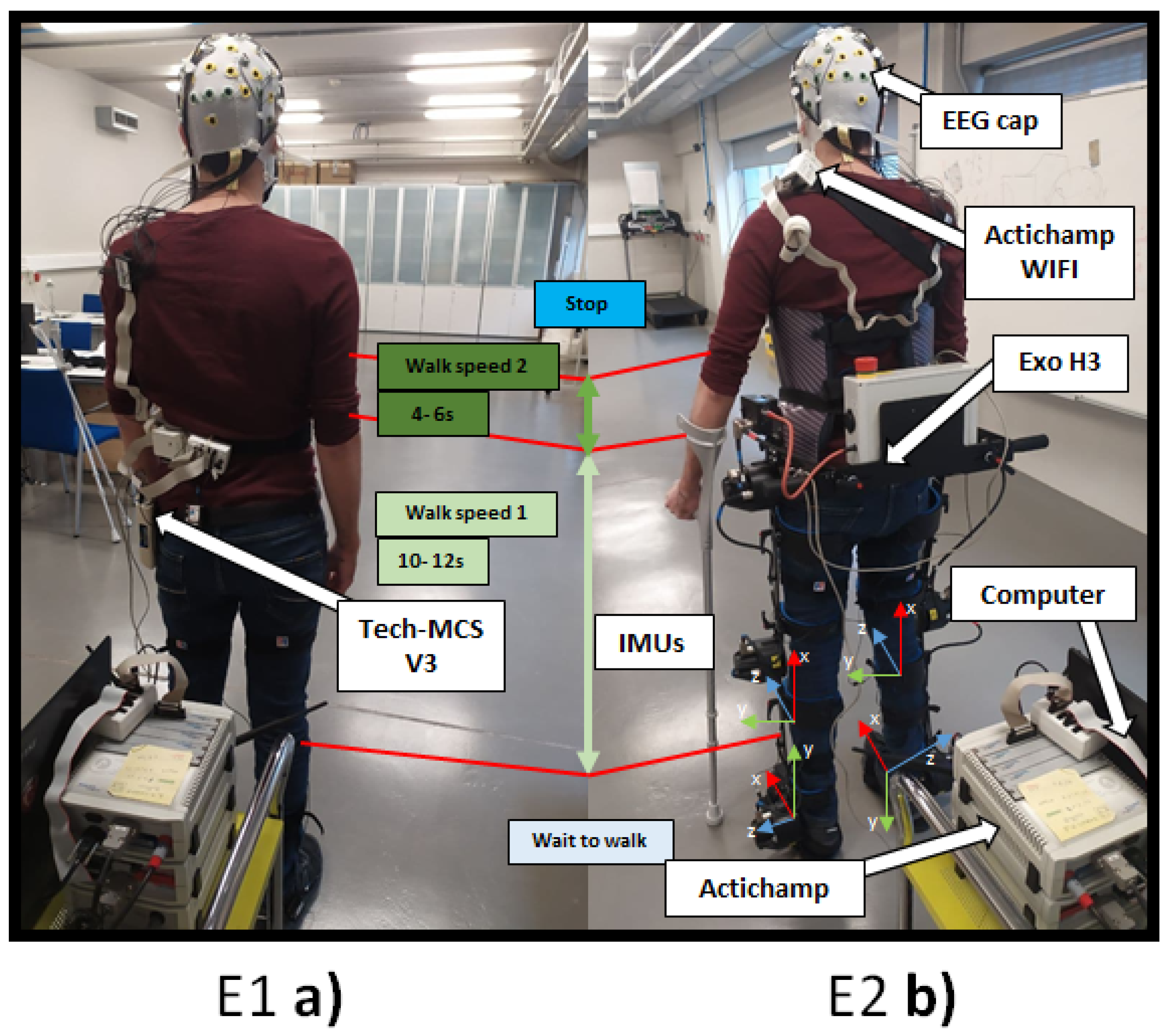
For the EEG data recording, a 32 electrodes system actiCHamp (Brain Products GmbH, Germany) was used (see Figure 1). Signals were transmitted wirelessly by a Move transmitter to the actiCHamp. The electrodes registered EEG activity through 27 noninvasive active electrodes following the international 10-10 system distribution (F3, FZ, FC1, FCZ, C1, CZ, CP1, CPZ, FC5, FC3, C5, C3, CP5, CP3, P3, PZ, F4, FC2, FC4, FC6, C2, C4, CP2, CP4, C6, CP6, P4). One of the electrodes was placed on right ear lobe for reference and an additional electrode acted as ground on the left ear lobe. The other 4 electrodes were placed to record electrooculography (EOG) activity in bipolar configuration (HR, HL, VU, VD). A medical rack was placed on the head to mitigate electrode and wire oscillation due to motion. Signals were registered at 500 Hz. Seven inertial measurement units (IMUs) (Tech MCS V3, Technaid, Spain) were placed for registering the walking parameters at 50 Hz sampling (Figure 1). Four of them, placed on shins and foots, were used for processing the actual speed change moment.

For the closed-loop experiment, an H3 exoskeleton (Technaid, Spain) was used to assist the user in the speed change intention.

2.3. Experimental Procedure Training

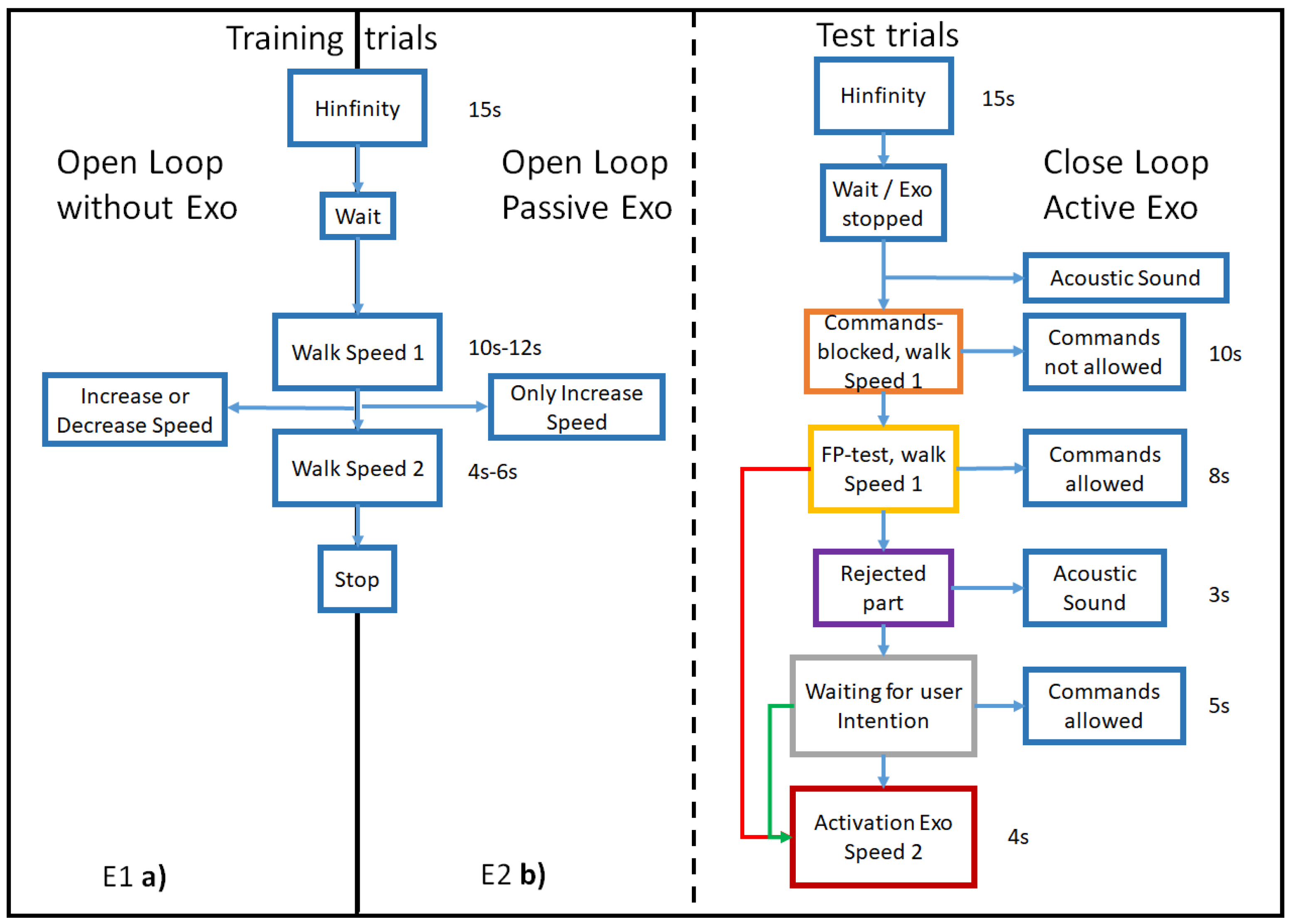
In this study, two protocols were used. In E1 (Figure 2a), data were recorded from five users in which EEG was collected in states of monotonous walk and change intention to subsequently analyze them in offline and pseudo online analysis. A second experiment E2, see (Figure 2b), was also recorded for the same two states while exoskeleton was controlled in closed-loop. E1 protocol was also used to obtain the training trials of the EEG classification model that would be used to control the exoskeleton in closed-loop. During these training trials the exoskeleton was in passive (non-assistance) mode.

In the training phase for both E1 and E2 the users performed the following process for each trial. First 15 s were used for $H^{\infty }$ convergence [19]. Then, they started walking at a constant speed during 10–12 s till a voluntarily increase or decrease of speed within a specified area (as a guideline) was performed, then speed was maintained between 4 and 6 s. The first two training trials were used to set the speed. This helps the subject to learn how to perform the increment within the delimited (but diffuse) area in a wide interval. It was emphasized that the subject did not think beforehand to make the change and that the view was always set forward. This was repeated 8 more times. During all the trials, a technical assistant followed the subject from behind with the acquisition equipment on a cart (Figure 1). As a result of the 10 trials, 80 speed changes were registered, with approximately an statistical distribution of 50% increases and 50% decreases.

2.4. Analysis IMUs

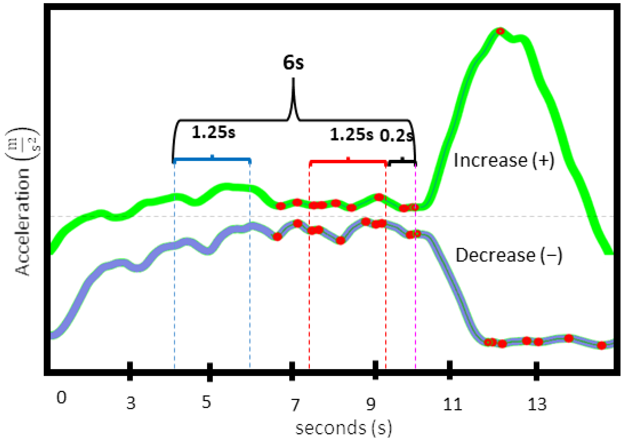
To create a predictive model that could detect the brain patterns associated with the intention of changing the walking speed, the registered EEG signal must be properly labeled according to the IMUs information (Figure 1). For the four selected IMUs, the calculation of the acceleration modulus the three axes were used: X, Y and Z. A moving mean (movmean in MATLAB) filter was applied to the four signals with a processing size equal to the IMUs sampling period and a three order Savitzky–Golay filter. The average of each signal was suppressed and the four signals were averaged. In order to label the speed changes, all peaks of the processed signal (findpeaks MATLAB function) were detected after the first six steps to avoid the first slope when the subject starts walking (Figure 3). The difference in amplitude between each point and the previous point was also computed. The first point of the maximum difference between peaks (see red points in Figure 3) was selected as the change instant. This value was resampled to the frequency sample of the EEG.

It was also detected when the first walking step was performed in each repetition, following a segmentation method [20].

To characterize the acceleration direction, the following rule was applied: If the maximum value of the repetition is twice the average of the first two seconds after the first step, it is labeled as Increase. If not, the repetition is labeled as Decrease.

2.5. Offline BMI

In this section, the methodology used to analyze the brain activity (recorded as the protocol methodology explained in Section 2.3) and create the model is explained. Previously to the recording, a high pass filter with a 0.1 Hz cutoff frequency and a notch filter at 50 Hz (remove power line interference) were applied by actichamp hardware. The preprocessing steps were applied sample by sample to the entirely signal. An adaptive artifact EOG removal algorithm $H^{\infty }$ [19] was used, the algorithm parameters were: $\gamma$ = 1.15, q = 1 × e${}^{-10}$, p0 = 0.5. Then, the EEG channel information was improved thanks to a Laplacian filter. Subsequently, a series of state variables butterworth band-pass filters of order 4 were applied to analyze different methods for the extraction of characteristics in these bands.

Next, the two different classes were segmented thanks to the IMUs information (check the procedure explained in Section 2.4). The speed change class consisted of the EEG data previous to the detected change point by the IMUs (pink line in Figure 3) between −1.45 to −0.2 s (avoiding taking the right moment in which the change is made). The walking class was selected between −6 to −4.75 s, where the person walks at a constant speed (Figure 3).

A repetition should be discarded if it did not comply any of the following premises:

• Something goes wrong during the protocol: some strange noise, unexpected event of the subject or detachment of the IMUs.
• Failure of IMUs algorithm: the algorithm of the IMUs did not correctly detect the moment of change. This could be easily detected by an algorithm that aligns the signals with respect to the tagged point.
• Time failure: there was not enough time between the algorithm detection of the start of the walk (the third step) and the area of change (>6 s). With this rule it was avoided that in the walking class there was information close to the first step.

On

Table 1. Number of valid repetitions of each subject for the three types of models/total repetitions performed for each type of model.

	Valid Repetitions
	Increase	Decrease	Both
S1	31/43	32/37	63/80
S2	45/48	31/32	76/80
S3	44/45	32/35	76/80
S4	45/46	34/34	79/80
S5	39/41	39/39	78/80

, the number of valid repetitions and total repetitions are specified by subject and each of the models considered: Increase, Decrease and Both.

2.5.1. Features

Temporal and frequency single features were extracted for each window class: The power spectrum density (PSD) (pburg in MATLAB):

$$S_{xx}\left(\mathrm{\Omega }\right)\sum _{m=-\infty }^{\infty }{R}_{xx}\left[m\right]e^{-j\mathrm{\Omega }m}$$

(1)

where $R_{xx}$ is the autocorrelation function that can be reconstructed from its power spectrum $S_{xx}\left(\mathrm{\Omega }\right)$, the PSD estimates the power distribution in each frequency band.

The Shannon entropy:

$$Shannon\hspace{0.17em}Entropy=-\sum _{i=1}^N{\left|C_i\right|}^2{\log }_e{\left|C_i\right|}^2$$

(2)

where N is the number of coefficients in the wavelet subband, $C_i$ is the wavelet coefficient having index i. The Shannon entropy measures the nonlinear properties of the signal, which indicates signal variation at each frequency scale, that could be related to the ERD/ERS process [21].

The first Weibull parameter:

$$y=f\left(x\right|a,b)=b{a}^{-b}{X}^{b-1}{e}^{-{\frac{x}{a}}^b}$$

(3)

where b is the scale parameter of the distribution and a is the shape parameter and X is a continuous random variable. The Weibull distribution has been used as an indicator of a physiological neural process [22,23].

The three Hjorth parameters, where y is the signal of one channel and t is the time:

Activity which represents the proportion of standard deviation of the power spectrum:

$$H{J}_A=var\left(y\left(t\right)\right)$$

(4)

Mobility which represents the mean frequency:

$$H{J}_M=\sqrt{\frac{var\left(\frac{dy\left(t\right)}{dt}\right)}{var\left(y\right(t\left)\right)}}$$

(5)

Complexity which represents the changes in frequency:

$$H{J}_C=\frac{Mobility\left(\frac{dy\left(t\right)}{dt}\right)}{Mobility\left(y\right(t\left)\right)}$$

(6)

Features were selected based on its common use in these type of studies [6,14,24] and the possibility of being used with only a few samples per class.

Each of the features were computed in the different bands extracted with the state variables band-pass filters: whole spectrum (8–40 Hz), alpha (8–14 Hz), low beta (15–22 Hz), high beta (23–30Hz), low gamma (31–40 Hz) and high gamma (41–60 Hz).

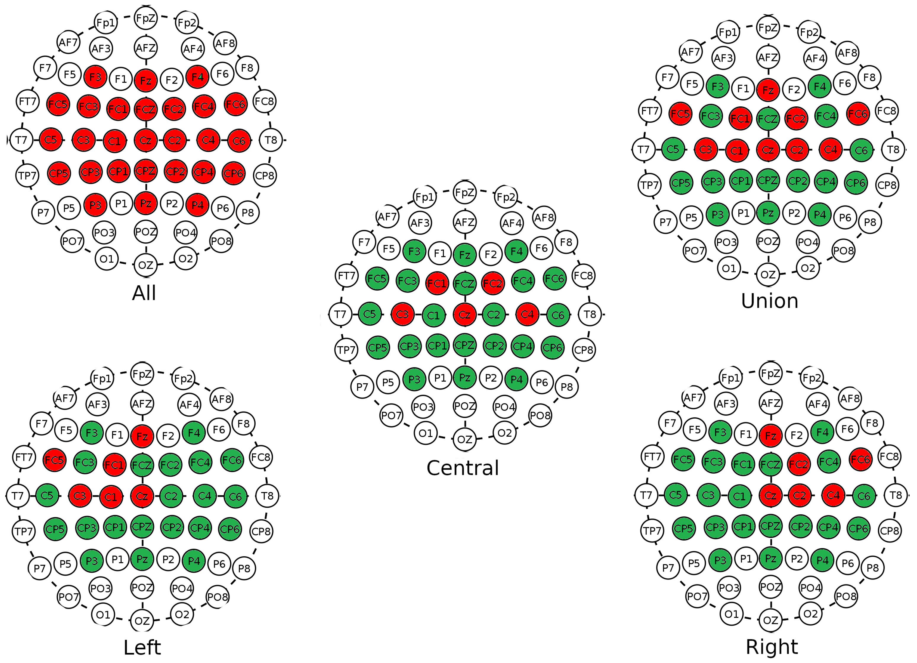
2.5.2. Electrode Selection

Each feature and model type combination was tested in the following electrode configurations based on supplementary, premotor and primary motor areas (see, Figure 4): All (27 electrodes); Union (Fz, FC2, FC1, FC6, FC5, FC5, Cz, C1, C2, C4, C3), Left (Fz, FC1, FC5, Cz, C1 and C3); Central (FC1, FC2, C3, Cz and C4); and Right (Fz, FC2, FC6, Cz, C2 and C4). These combinations were chosen based on studies that compared these combinations under similar conditions [25].

2.5.3. Cross-Validation and Feature Selection

In this section, the proposed features and electrode configurations were tested in order to check its capacity to detect the change of speed intention. This was done considering three conditions: a model with both speed changes as a common class (increase and decrease repetitions all together) vs. common speed walking state; and splitting the model for increase vs. common speed walking state and decrease vs. common speed walking state. The binary linear svm classifier (with a radial basis function kernel) was employed to obtain the accuracy percentages of a k-fold cross validation. Each of the models (Increase, Decrease or Both) was created with the repetitions considered as valid (see Table 1) minus those used for testing, which were always eight. The class walk was labeled as 0 and the class change was labeled as 1. Depending on the result of the binary classifier, each repetition was marked as a true or false event detection. Percentages of the total accuracies for walk and change speed classes (Equation (7)) were computed. In addition, the balance index (Equation (8)) related to the accuracy of both classes was assessed.

$$Acc=\frac{\mathrm{Number}\mathrm{of}\mathrm{true}\mathrm{event}\mathrm{detection}}{\mathrm{Number}\mathrm{of}\mathrm{total}\mathrm{event}\mathrm{detection}}$$

(7)

$$balance=abs\left(\frac{Acc\hspace{0.17em}Class\hspace{0.17em}Change-Acc\hspace{0.17em}Total}{Acc\hspace{0.17em}Class\hspace{0.17em}Change}\right)$$

(8)

To evaluate which were the best single features, 540 different configurations were tested for each of the five subjects: three types of classification models (Both, Increase and Decrease), six features, five electrode setups and six frequency bands. Only the results over 10 for both indices, accuracy and balance (Equations (7) and (8)), were considered as acceptable. The minimum value of accuracy to consider the model was acting over randomness was established according to the paper [26]. The threshold (Equation (9)) depends on the number of available samples (80 repetitions minus those neglected, Table 1). Results of each feature in each band that exceed this threshold have been averaged regardless of model classification, electrode combinations or subject (not all the configurations met the criteria). Then, a selection of features were done according to two criteria: number of times the features in the specific band was selected per user greater than the mean; and if the average percentage result was over the median of values. With these conditions, six features in different bands were selected.

$$Randomness\hspace{0.17em}Level=0.5+1.96\times \sqrt{\frac{0.5_{}^2}{Number\hspace{0.17em}of\hspace{0.17em}Valid\hspace{0.17em}Repetition+4}}$$

(9)

After this selection, to improve the classification performance based on individual features, all possible combinations with 6 individual features were carried out 2 in 2 to evaluate if more information by window could improve the results. This produced 15 combinations that were evaluated for the three types of classification models (Both, Increase and Decrease) and the 5 electrode configurations. In total, 150 combinations were tested for each user.

2.6. Pseudo-Online BMI

Once detected the best combination of features and electrode configurations for the three types of classification models, the pseudo-online analysis was performed in order to check them in a simulated real-time scenario.

No cross-validation was used in the pseudo-online analysis in order to simulate the real-time conditions. This way, the model was created using the first eight trials with the explained offline procedure and tested with the last two trials of each session with the following procedure.

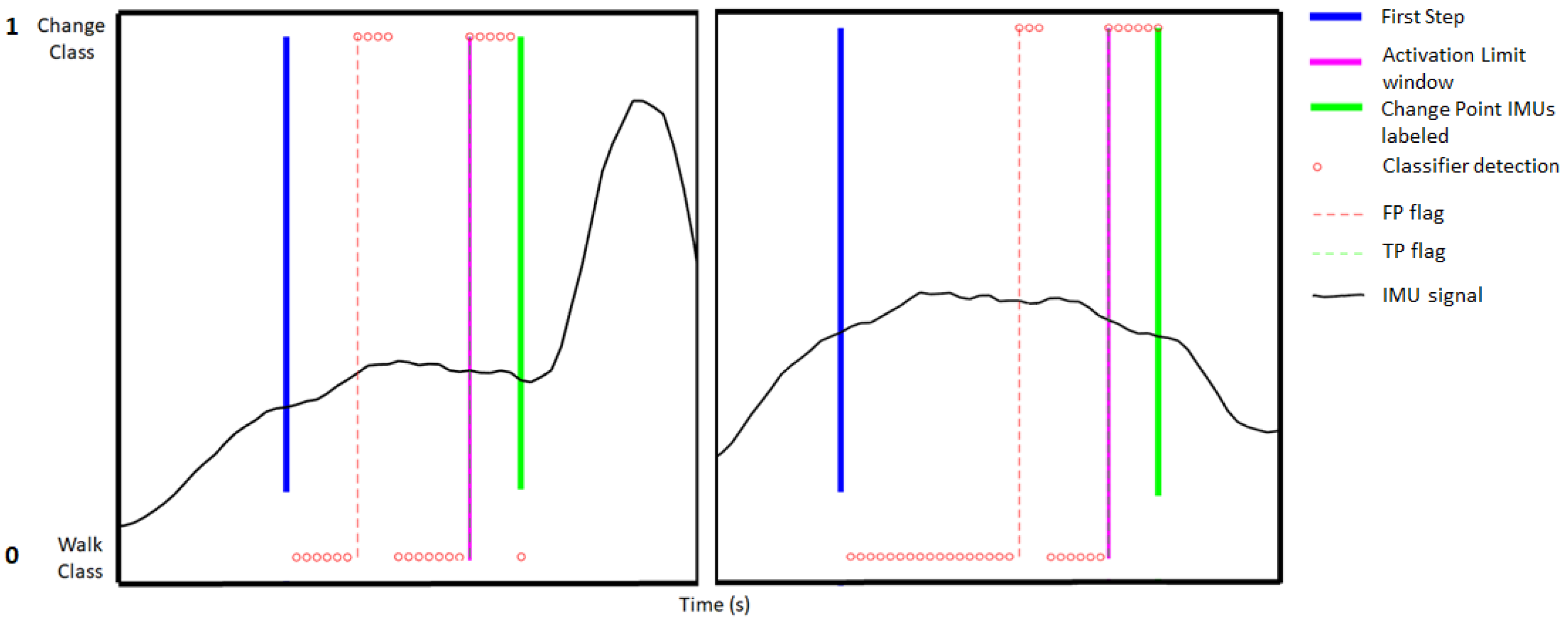
Trials were analyzed epoch by epoch, with a size of 625 samples (1.25 s), shifting them every 100 samples (0.2 s) producing an effective 1.05 s overlap between epochs. The preprocessing was done in the same way as in the offline model with the state variable filters. However, in the pseudo-online analysis, the whole signal was processed, extracting the features based on the electrode configuration that maximized the results (tested in Section 2.5.3) and for each of the models (Both, Increments and Decrements). Meanwhile, the classification of each window was only evaluated in the interval between points marked as the beginning of walking and the change labeled (see Figure 5). Regarding the command decision, a TP was computed if five consecutive epochs were identified as a speed change class and the detection was detected at most one second before the actual IMUs detection of the change, otherwise it would be considered as a FP. Taking into account the epoch size and shifting, the time window in which a TP can be considered valid before the actual change contains information from [−2.25 s,−1.25 s] to [1.25 s,−0.2 s] previous to the change.

The number of successful changes, i.e., the TP rate of the test, could be defined as:

$$\mathrm{TP}=\frac{\mathrm{Number}\mathrm{of}\mathrm{true}\mathrm{event}\mathrm{detections}}{\mathrm{Number}\mathrm{of}\mathrm{true}\mathrm{events}}$$

(10)

If one of the epochs was detected within the change range, a true event was computed and the signal processing was stopped until the start of the next repetition. As a realistic way to compute FP, once one was detected, the next one could not be computed until at least two seconds passed. This helps to simulate that in a real-time scenario, as the command is sent (to perform a feedback action), it is necessary to wait a while until the next command can be sent again. As the normal walking time period has a duration of 8–10 s, the FP evaluation can be expressed as:

$$\mathrm{FP}\min =\frac{\mathrm{Number}\mathrm{of}\mathrm{false}\mathrm{activations}}{\mathrm{walking}\mathrm{time}\mathrm{windows}\mathrm{in}\mathrm{minutes}}$$

(11)

Moreover, a ratio of TP to FP/min was computed. The higher the value of the ratio, the better the evaluation. The value of the variable ratio is equivalent to the number of $\frac{\mathrm{TP}}{\mathrm{FP}/\min }$.

2.7. Closed-Loop BMI

The subject that achieved the best TP/FP ratio at E1, participated in the pilot closed-loop experiment of the H3 exoskeleton (E2). The experiment only contemplated the intention of increasing speed. The H3 exoskeleton was used in two modes of assistance:

• Passive mode: It was used to create the model. The exoskeleton joints followed the user’s gait pattern with zero torque compensation, so they had to make a significant physical effort. In this mode, the user must walk at a constant speed and will change to their own will.
• Active mode: It was used during closed-loop control in which the exoskeleton started at a slow speed and when the BMI detected the intention of speed changing through EEG decoding, a command was sent to the exoskeleton to increase its speed.

To create the model, the register methodology was described in Section 2.3. The subject started walking in passive mode and at a certain moment the speed was increased voluntary by them. The IMUs were used to label the processing times in the same way than in E1 (see Section 2.4). No modifications were applied for the IMUs segmentation algorithm between the normal walk and the exoskeleton walk.

Signals were filtered and features extracted as in Section 2.5 was mentioned. The classification model was created with 32 of the 40 repetitions recorded in passive mode, as eight were discarded following the E1 rules. For the signal evaluation of the closed-loop test, the process was similar to the one explained in Section 2.6.

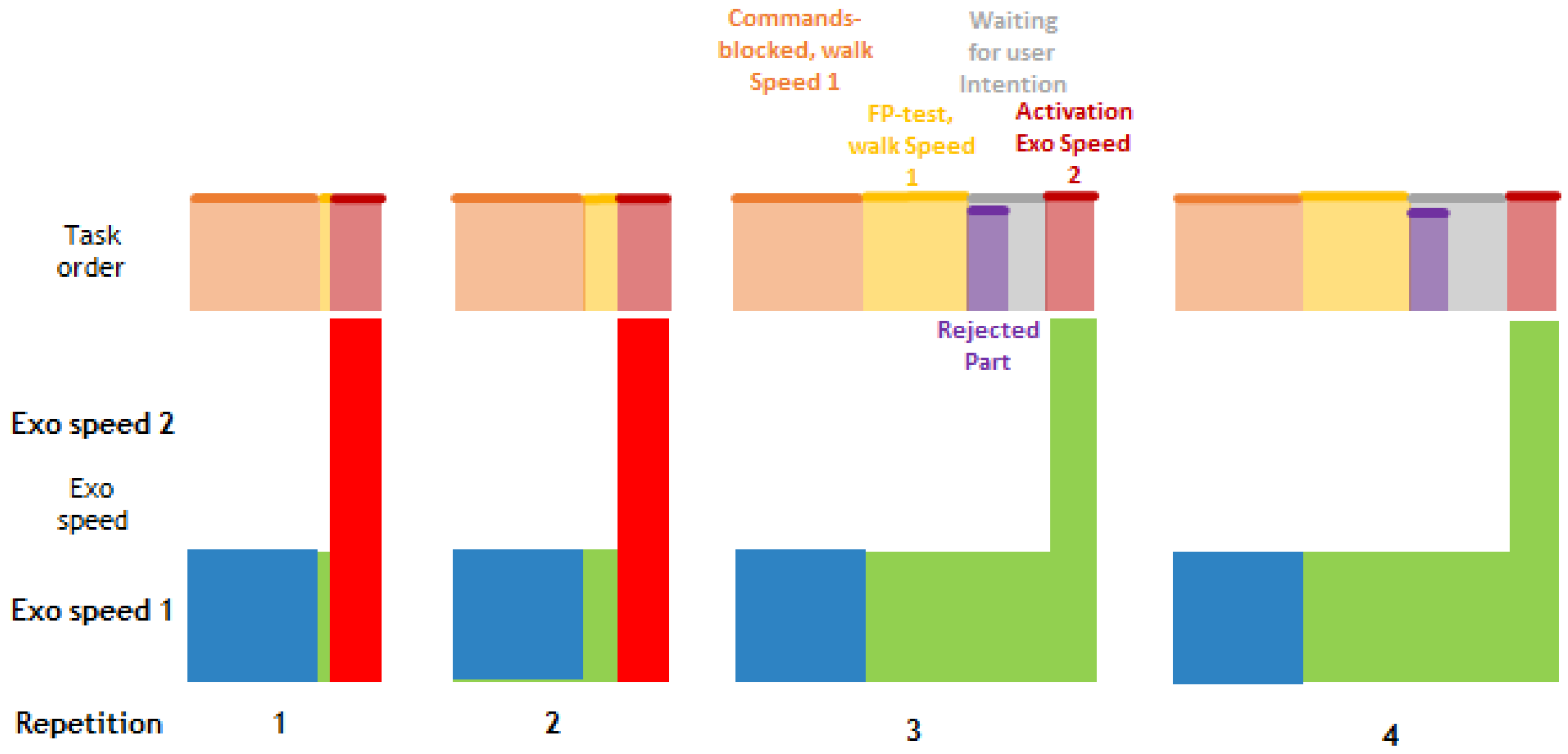
The detailed protocol for the closed-loop trials (see Figure 2b)) can be summed up as:

• 15 s of $H_{\infty }$.
• High-pitched sound warns the user 1s before the activation of the exoskeleton.
• The exoskeleton activates at speed 1 (0.8 m/s) and no commands are allowed for 10 s.
• After that, the FP evaluation starts. During 8 s at speed 1 the BMI can send commands to increase the speed depending on the brain activity.

  -

  If one FP is detected, the BMI sends to the exoskeleton the change of speed command during 4 s and returns to Wait/Exo stopped. If during this phase there are no FP, an auditory signal indicates the start of user intention validation. The subject was told that after the auditory signal they should wait at least 3 s before attempting the change at their own will. In this period the BMI does not allow commands to avoid the influence of the evoked potential.

• For the last 5 s, if a change is detected, the exoskeleton receives the command and increases its speed to 2 (1.1 m/s) for 4 s and then stop the exoskeleton. The protocol can be seen at Figure 2.

The exoskeleton activation time was extended from the theoretical 2 s considered at pseudo-online analysis to 4 s, as it was necessary in order for the subject to notice the difference in change between speed 1 and 2.

3. Results

The results of each of the tests and experiments presented above will be described in detail below.

3.1. BMI Offline

3.1.1. Feature Selection Methodology

As specified in the previous section, 540 configurations were tested for Both, Increase and Decrease classifier models. As it was mentioned in Section 2.5.3, those that met the indicated criteria were used to analyze the most relevant features to differentiate the searched potential: a feature is chosen if it is present for at least three subjects (value between brackets in

Table 2. Average of the accuracy of the features that among all the models exceeded the established thresholds. In parentheses is shown the number of users it appeared. Selected features are in bold. If they did not pass the inclusion criteria, it was indicated with “-”.

	8–40 Hz	8–14 Hz	15–22 Hz	23–30 Hz	31–40 Hz	41–60 Hz
Pburg	-	64.6 (1)	58.9 (1)	-	-	-
EShnn	58.3 (1)	64.1 (1)	-	61.8 (1)	64.5 (2)	-
WP	68.7 (2)	64.5 (2)	61.8 (3)	60.9 (2)	63.2 (2)	63.7 (1)
HJ${}_A$	61.6 (1)	65.2 (3)	62.7 (2)	63.0 (3)	68.4 (2)	61.1 (1)
HJ${}_M$	63.9 (1)	64.2 (3)	64.8 (2)	64.6 (1)	61.6 (2)	58.3 (1)
HJ${}_C$	59.8 (1)	63.0 (3)	63.8 (4)	63.6 (4)	61.8 (2)	61.9 (3)

) and its average accuracy is over the median (63%). Using these criteria, six values were chosen. The chosen features and bands configurations are highlighted in bold in Table 2: $H{J}_A$ in band 8–14 Hz and in band 23–30 Hz, $H{J}_M$ in band 8–14 Hz, and $H{J}_C$ in band 8–14 Hz, 15–22 Hz and 23–30 Hz. Pburg, Shannon and Weibull were the features with the lower accuracies. Temporal features were much more effective than frequency features.

Averaging the band values in Table 2 for each feature, the band with the highest percentage and the one that appeared the most was 8–14 Hz with a ratio of 2.16 and a percentage of 64.24% being the second band 23–30 Hz with 53.31% and a ratio of 1.8.

For all the results that passed the acceptance criteria, a statistical analysis was carried out to analyze differences between the model types: Both, Increments and Decrements, and if there were differences between subjects:

• Model type in terms of average accuracy: Since data of each methodology did not follow a normal distribution, as assessed by Shapiro–Wilk test, Kruskal–Wallis test was used. It showed that the performance was different based on the methodology (p-value < 0.05). Post-hoc analysis revealed statistically relevant differences between both increments and decrements (p-value < 0.05).
• Subject difference in terms of performance: Shapiro–Wilk test was applied to assess the normality assumption of ANOVA. Data of every subject did not show a normal distribution (p < 0.05), so Kruskal–Wallis test was employed. Results from this test showed no significant differences among subjects (p-value > 0.05).

3.1.2. Cross-Validation Analysis of Electrode Configurations and Combined Features

Among all the configurations tested and specific to E1, the best results for Single features of the six selected and Combination features are shown in

Table 3. Comparative table of best results according to feature selection. The table compares the best results for total accuracy depending on the paradigm and electrode configuration as Single or Combined (Comb) for the offline analysis.

		Both			Increase			Decrease
		Feat.	Chan.	Acc.(%)	Feat.	Chan.	Acc.(%)	Feat.	Chan.	Acc.(%)
S1	Single	$H{J}_A$	Union	63.4 ± 16.7	$H{J}_A$	All	68.8 ± 10.2	$H{J}_A$	Union	58.3 ± 9.5
		(8–14)			(8–14)			(23–30)
	Comb	$H{J}_A$	All	67.0 ± 8.6	$H{J}_A$	All	70.3 ± 10.7	$H{J}_A$	Left	66.7 ± 19.1
		(8–14)			(8–14)			(23–30)
		$H{J}_A$			$H{J}_C$			$H{J}_C$
		(23–30)			(8–14)			(8–14)
S2	Single	$H{J}_M$	Central	59.0 ± 14.4	$H{J}_C$	Central	64.6 ± 7.2	$H{J}_M$	Union	54.9 ± 11.2
		(8–14)			(23–30)			(8–14)
	Comb	$H{J}_A$	Union	64.6 ± 12.5	$H{J}_C$	Central	77.1 ± 3.6	$H{J}_A$	Union	65.0 ± 9.5
		(23–30)			(15–22)			(23–30)
		$H{J}_C$			$H{J}_C$			$H{J}_C$
		(15–22)			(23–30)			(15–22)
S3	Single	$H{J}_A$	All	66.7 ± 8.3	$H{J}_A$	All	67.2 ± 11.8	$H{J}_A$	All	62.5 ± 11.7
		(23–30)			(23–30)			(23–30)
	Comb	$H{J}_A$	All	68.1 ± 8.5	$H{J}_A$	All	71.9 ± 13.0	$H{J}_A$	All	65.0 ± 11.4
		(23-30)			(23-30)			(8-14)
		$H{J}_C$			$H{J}_C$			$H{J}_C$
		(8–14)			(15–22)			(15–22)
S4	Single	$H{J}_C$	All	58.3 ± 13.6	$H{J}_A$	All	67.2 ± 13.9	$H{J}_C$	Left	58.8 ± 7.1
		(15–22)			(8–14)			(15–22)
	Comb	$H{J}_C$	Left	66.0 ± 10.4	$H{J}_A$	Central	71.9 ± 6.3	$H{J}_C$	Left	60.0 ± 10.5
		(15–22)			(8–14)			(15–22)
		$H{J}_C$			$H{J}_C$			$H{J}_C$
		(23–30)			(23–30)			(23–30)
S5	Single	$H{J}_A$	Left	64.6 ± 13.6	$H{J}_A$	Left	68.8 ± 7.2	$H{J}_C$	Right	67.2 ± 17.2
		(23–30)			(23–30)			(15–22)
	Comb	$H{J}_A$	Left	64.6 ± 13.6	$H{J}_A$	All	73.4 ± 9.4	$H{J}_M$	Right	67.2 ± 17.2
		(23–30)			(23–30)			(8–14)
		$H{J}_M$			$H{J}_C$			$H{J}_C$
		(8–14)			(8–14)			(15–22)

for each model type (Both, Increase and Decrease) and in different electrode configurations, depending on the feature.

The values for the Combination features are higher than the Single features in general for each of the subjects and classifier models. For the average of subjects and models, Single features show an average accuracy of 63.3 ± 11.6%, while the Combination of features shows a better average value of 67.9 ± 10.9%. The largest difference between Single and Combination accuracies across subjects is shown in the model that uses only the Increase class with a difference in accuracy of 5.6%. This difference is in Decrease of 4.4% and in Both of 3.7%. The Combination configurations increase the results in all conditions, the average improvement was 4.6%

The highest accuracy (see, Table 3) and the lowest standard deviation comparing Combination and Single feature classification in user average is shown in the Combination configuration for the Increase model, 72.9 ± 8.6%. In second place Both 66.1 ± 10.7% and lastly Decrease 64.8 ± 13.5%.

Regarding the electrode configurations, the ratio of appearance of the computed configurations in Table 3 is as follows: the All electrode configuration appears 12 times, the Left appears 7 times, the Union appears 5 times, the Central appears 4 times and the Right appears 2 times. Based only on the Combination features, the Central electrode configuration, with an appearance ratio of 2, has an accuracy of 74.5%, while in second place the All, with an appearance ratio of 5, has an accuracy of 68.5%. The All electrode configuration is the most repeated in the Both and Increase models among all subjects and regardless of Single or Combination: it appears in Increase 6 times and in Both 4. In Decrease the Union electrode configuration is the most popular and appears 3 times.

The band that appears the most in Table 3 is 23–30 Hz with a total of 19 times. The 8–14 Hz is selected 15 times, less than the 23–30 Hz even though 3 features are selected from the 8–14 band in the feature preselection (see Table 2). The one that appears the least was 15–22 Hz, a number of 11 times, but only 1 feature ($H{J}_C$) is selected in this band in the preselection (see Table 2).

The $H{J}_A$ feature is selected in Table 2 in fewer bands than the $H{J}_C$. However, going back to Table 3 and putting together the times, $H{J}_A$ appears in Single 9 and in Comb 12 times for a total of 21 times, slightly more than $H{J}_C$ that appears a total of 20 times. $H{J}_C$ is the second in appearance, with a high difference between the 16 times it appears in Comb and in Single, only 4. $H{J}_M$ is by far the one that appears the least with only 4 times, 2 in single and 2 in Comb.

Regarding how the bands are distributed in the features (see Table 3): $H{J}_A$ between Single and Comb has more representation in the 23–30 Hz band than in the 8–14 Hz band. The $H{J}_C$ setting appears mostly in the 15–22 Hz band.

Regarding how the features are combined in Comb: $H{J}_A$ in combination with $H{J}_C$ are the ones that appear the most for a total of 9 times, while $H{J}_C$ with $H{J}_C$ appear three times. Other combinations appear only once, except $H{J}_M$ and $H{J}_M$ that has no appearance.

In summary, the $H{J}_A$ feature is the most representative feature in Single. When it is combined it appears a lot in combination with the $H{J}_C$. There is no significant combination of these on fixed bands, however the $H{J}_A$ setting at 23–30 Hz and $H{J}_C$ at 15–22 Hz appear repeated 3 times as $H{J}_A$ at 23–30 Hz and $H{J}_C$ at 8–14 Hz which also appear 3 times.

Based on the results, the Combination of features was chosen for the pseudo-online assessment. The features chosen were those shown in Table 3, 2 features each per band and in different electrode configurations.

3.2. Pseudo-Online Results

The best combined feature configurations computed in offline methodology were tested in pseudo-online validation, but with a different computation procedure as described in Section 2.6. In

Table 4. Pseudo-online results per user showing TP, FP/min and ratio ($\frac{\mathrm{TP}}{\mathrm{FP}/\min }$) for the best Comb (calculated in the offline analysis) feature and electrodes combination for Both, Increase and Decrease paradigms.

		S1	S2	S3	S4	S5
Both	Features	$H{J}_A$ (8–14)	$H{J}_A$ (23–30)	$H{J}_A$ (23–30)	$H{J}_C$ (15–22)	$H{J}_A$ (23–30)
		$H{J}_A$ (23–30)	$H{J}_C$ (15–22)	$H{J}_C$ (8–14)	$H{J}_C$ (23–30)	$H{J}_M$ (8–14)
		All	Union	All	Left	Left
	TP(%)	40.0	50.0	37.5	18.8	25.0
	FP/min	11.1	10.5	5.0	8.2	4.6
	ratio	3.6	4.8	7.5	2.3	5.4
Increase	Features	$H{J}_A$ (8–14)	$H{J}_C$ (15–22)	$H{J}_A$ (23–30)	$H{J}_A$ (8–14)	$H{J}_A$ (23–30)
		$H{J}_C$ (8-14)	$H{J}_C$ (23–30)	$H{J}_C$ (15–22)	$H{J}_C$ (23–30)	$H{J}_C$ (8–14)
		All	Central	All	Central	All
	TP(%)	42.9	55.6	33.3	33.3	62.5
	FP/min	9.9	17.9	5.6	3.8	9.1
	ratio	4.3	3.1	5.9	8.8	6.9
Decrease	Features	$H{J}_A$ (23–30)	$H{J}_A$ (23–30)	$H{J}_A$ (8–14)	$H{J}_C$ (15–22)	$H{J}_M$ (8–14)
		$H{J}_C$ (8–14)	$H{J}_C$ (15–22)	$H{J}_C$ (15–22)	$H{J}_C$ (23–30)	$H{J}_C$ (15–22)
		Left	Union	All	Left	Right
	TP(%)	37.5	57.1	71.4	28.6	28.6
	FP/min	15.5	12.3	15.5	10.0	7.7
	ratio	2.4	4.6	4.6	2.9	3.7

, the pseudo-online results metrics are shown for each subject.

On average, the TP for the three types of models were for Both: 34.4%, Increase: 45.5% and Decrease: 44.6%. The average FP/min was for Both: 7.9, for Increase: 9.26 and for Decrease: 12.2. The average TP vs. FP ratio were for Both: 4.3, Increase: 4.9 and for Decrease: 3.6. Although the differences are not very significant, the Both paradigm presents the lowest FP of the three models and the one that shows the worst performance is Decrease. On average, the model that achieved the highest value of TP and FP/TP was the one that used only the Increment model.

Pseudo-online results were not equivalent to those shown in offline. The best configurations per user in offline mode were not analogous to the best configurations in pseudo-online mode. For instance, user S2 showed an offline accuracy for the Increase model of 77.1 ± 3.6%, but the same setup tested in pseudo-online obtained the highest FP/min with 17.9.

3.3. Exoskeleton Closed-Loop

The subject that obtained the best results in the pseudo-online analysis was S4, with the combination of $H{J}_A$(8–14)/$H{J}_C$(23–30) features, the central electrodes configuration and a ratio of 8.8. This was the reason why it was selected for the pilot test E2.

The E2 concept study was performed two weeks after the first E1 study. In E2, 40 repetitions of increment of the speed of the exoskeleton in passive mode were carried out during the first phase for training the model, five trials of eight repetitions. For the creation of the model, the first trial was ruled out, since the user was adapting to the use of this mode. Thus, the model was created with 32 repetitions.

Regarding the testing with the exoskeleton in active mode, only six closed-loop repetitions were performed due the user fatigue and to limit experimental duration. The training process was long, the subject had to perform a lot of force to move the exoskeleton in passive mode, being its control complex. This caused the experiment to be longer than expected and the cause of the closed-loop repetition shortening.

Of the six repetitions performed in a closed loop, in the first 2, a false positive was detected in the validation stage FP-Test (see Figure 6) 0.2 s and 3.4 s, respectively, after the Commands-blocked, walk Speed 1 phase (see

Table 5. Differences in seconds between FP-test task start and false positive activation and between waiting user intention task start and activation of speed command 2 for the FP and TP cases.

		Repetition 1	Repetition 2	Repetition 3	Repetition 4	Repetition 5	Repetition 6
	FP-test, walk Speed 1	0.2 s	3.4 s	-	-	3.2 s	1.4 s
	Wainting user Intention	-	-	2.8 s	3.8 s	-	-

), while in the next two there were no FP in the validation stage and in the waiting for user intention stage, 2.8 s and 3.8 s, respectively, after the rejected part stage was activated correctly according to the user’s intention. In repetitions 5 and 6, as in repetitions 1 and 2, 3.2 s and 1.4 s were activated incorrectly after starting the stage.

Counting the time that it was active without false activation and the total of 4 false activations, the false positives in the 6 repetitions added up to a total of 9.92 FP/min, while the number of TP was 33%.

4. Discussion

In this section, the peculiarities of previous works have been reviewed, in order to analyze which are the factors that differentiate our work and what can be interpreted from our results. The decoding of movement intention through EEG has been analyzed in the bibliography attending to four criteria:

• The time window of the EEG information used. The intention has been analyzed only with data signal before the point labeled as beginning of the movement [6,11,12,13,14,15] or also data signal during and after it [10,17].
• Analysis of the cerebral activity to study the paradigm in asynchronous (offline, pseudo-online) or synchronous (online) processing [13,15]. Asynchronous processing studies simulate the control of the rehabilitation/assistive device in open-loop while synchronous BMIs can control it in open or closed-loop.
• Most EEG-based intent studies show an analysis of brain activity without taking into account the implementation part of the BMI, which requires a closed-loop analysis with visual or auditory feedback [27] or sensitive motor feedback provided by an assistive control devices [13,15].
• Level of planning in which the movement was attempted: some studies establish an acoustic cue or mark when the subjects should perform the intention [15,16,28], other determine a planning period based in visual cues in which the users take the decision to perform the action [11,17], while other perform the action by their own will within a region limitation, like in this study [14], or with less conditions [10,12,29].

There are not many studies that analyze the intention in a task that switches from motion to motion, and those that analyze in the MRCP band can be greatly compromised by low-frequency artifacts. In this study, it has been reported the feasibility of decoding the user intention at bands combinations 8–14 Hz, 15–22 Hz and 23–30 Hz in speed changes for either Increase, Decrease or Both. The closed-loop control is not yet reliable enough to create an interface capable of assisting or designing rehabilitation therapies focused on patients. To address this problem, this work has proposed an interface with protocols capable of operating in real time and producing decision making according to the user’s intention in some of the cases. Some of the key aspects of this work will be discussed below.

4.1. Offline Cross Validation

In this work, temporal descriptors have been used for feature extraction versus frequency descriptors due to their better performance. Other works [6] have explored these Hjorth descriptors with different windowing methodologies that in our opinion might not be suitable for a closed-loop real-time test.

Regarding offline analysis and feature selection, as shown in Table 2, the Hjorth features are the most relevant, being the bands that contribute the most those in the ranges between 8 and 14, 15–22 and 23–30 Hz. These bands had more configurations that passed the average level of randomness and therefore, they are significant for the distinction of both classes.

The two most selected features in the table were $H{J}_C$ and $H{J}_A$. Both describe frequency behaviors but in the time domain. The first one, as explained in Section 2.5.1 section, offers a comparison of the signal with a pure sine wave function. While $H{J}_A$ indicates the average power of the signal. The temporal characteristics impose on the frequencial ones.

Table 3 specifies the best Single and Combination features: the most relevant feature in the frequency band and in the electrode configuration. According to these results, the offline analysis shows a better accuracy of the Increase model. In this model, the best single features are preserved in combination and maximize the value in combination with the $H{J}_C$ band in some of its bands. The All and Left electrode configurations are the most relevant for this model.

4.2. Pseudo-Online

The pseudo-online model does not perform as well as expected. TPs are low because the chosen rule is restrictive, this design rule seeks to reduce FP. In this study, the TPs were lower than the mean of results found in the literature. However, those studies that carry out a real-time implementation tend to reduce TP in order to achieve less FP: in Bai et al. [27] a classifier working point was chosen in which the TPs were below 40% and this is not an impediment to the operation of the interface.

The FP/min in this study in comparison with the literature for intention ERD/ERS paradigms are similar. In addition, studies that use only information from before the event tend to have more FP/min for start 6.8 ± 0.7 and stop 9.4 ± 1.0 [12] that those which use before and after information, e.g., FP/min for start 3.5 ± 1.8 and for stop 2.1 ± 1.1 [10]. However, as indicated in the introduction, using only information prior to the change may be more interesting for the assistance process. This is because it does not contain information associated with the movement, only the intention.

However, in this study, the results of the increment interface were acceptable, which presents it as a viable tool. Large differences have been found between the results of the offline and online models, which may indicate that the characteristics belonging to the intermediate times between these two classes may be similar to those of the change class. Therefore, further work is needed in order to have a better classifier model.

Nevertheless, the results are not good enough for an interface in the clinical scenario. However, exploring different metrics and different ways of assessing the walking state variability could improve the reliability of the model.

4.3. Closed-Loop

Finally, the approach of our online closed-loop study shows the feasibility of creating an interface for speed gait control. Two of the trials exceeded 8 second intervals without showing false positives. The subject’s concentration and state may be a key factor, as well as the degree of experience in the use of a BMI like the one presented. There are few online lower-limb studies. Referring to upper-limb, in [27], the differences between pseudo-online and online analysis for open-loop control are shown. The research uses the ERD/ERS paradigm for the wrist movement. Great variations are observed between the validated model in pseudo-online, as TP was kept under 0.4 and FP close to 0, an the online experiments, where 60% of the trials obtained FP and 75% of the predictions were performed correctly, which indicates that lots of positive detections were obtaiend by the classifier. There are not many comparable studies for lower-limb in closed-loop methodology that use the ERD/ERS paradigm. In [13], the start–stop model achives TP of 89% and 8 FP/min in pseudo-Online analysis, while the closed-loop gets TP of 92% and 28 FP/min.

This difference between types of analysis is also noticeable in our study. Although the distribution of the FPs allowed the 8-second stage to be exceeded in two of the 6 repetitions, the number of FP/min was 9.92, higher than expected. However, the number of TPs remained within the values expected from the pseudo-online model with a 33%. Mental states of expectation could influence real-time decoding. The source and solution of the differences between offline analysis with pseudo-online control and online processing with closed-loop control is a problem to be explored and discussed in future publications.

4.4. Study Limitations

The manuscript presents a novel study for the prediction of the intention to change speed by EEG analysis. The final objective is to assess the viability of a real control of assistive mobility devices. Nevertheless, it is important to remark that this is a preliminary study with some limitations.

The database is formed by five subjects, which, although it may be short, it is kept within the ranges of other studies. Even though, the results of the offline model are acceptable, the results of the pseudo-online methodology are not equivalent and completely consistent. New window segmentation methods could be better suited to characterize the classification model used in the pseudo-online test.

• Try a moving window, to better represent the Walk class.
• Subdivide in smaller windows, to have a window that better represents the classes, at the cost of introducing more variance in the analysis window, since the ERD/ERS pattern could vary throughout the subdivided windows.
• Test a representation of the unbalanced walk class.
• Test another continuous decoding classifiers, such as GMM or a decomposition of components with some threshold limits. Decomposition methods like EMD could not be valid for real-time processing, but eigendecomposition [30] or cwt decomposition components could.

An important point in the development of a real-time experiment is that once the training is done, the model must be created in an acceptable time. This becomes even more important when this is validated on patients. The creation of a pre-selection of features could speed up the process. These pre-selected features can be optimized and their combinations customized. In this preliminary study, a pre-selected group of features were chosen.

Regarding the BMI efficacy, the number of false positives in this study is close to other studies in similar conditions. The exoskeleton closed-loop control experiment shown presents a concept study. From the experience of this pilot test, several consequences can be extracted. First, the reduced number of test repetitions was due to the fact that using the exoskeleton training methodology in passive mode results in a tiring process. Decreasing the number of trials may be an option. Three protocol alternatives could be used to train the model:

• In the first one, the model would be trained with the exoskeleton running in two speeds that would be changed when the exoskeleton gauges register a change. This needs, further research to be carried out.
• In the second one, the model would be trained with the exoskeleton running at two speeds and the user would be the one who would indicate the change by means of a button when they wants to change the speed. This could condition the EEG potential, due to the different states of consciousness.
• In the third, the model would be created without an exoskeleton and later the closed-loop would be made with an exoskeleton. This could reduce the subject’s fatigue, but could generate training vectors too differenct with respecto to the testing ones.

As the ultimate goal is to improve assistance, reducing FPs is a priority issue. To this end, more realistic models that represent better the data must be addressed. All of the above is important for this. In addition, new feature extractions should be explored, optimizing the filters that could improve the signal to noise ratio. There is not much exploration on the usefulness and differences between noise filters as $H_{\infty }$ or ASR depending on what kind of potentials are decoded.

5. Conclusions

A brain–machine interface for the classification of EEG signals related to intention process and speed changes in real time has been proposed. The model for the class intention has been trained with only information from the moments before the change. First, data were analyzed in offline cross-validation and in a simulated real time analysis (pseudo-online). The best features were selected in a generic way to describe the intention paradigm. Second, a real-time proof of concept with the exoskeleton was designed. It allowed to control the increase of speed of an exoskeleton in real time, and to validate the feasibility of the previous study in a realistic way.

The study has concluded that the Hjorth parameters are viable for decoding the intention of speed changes. Among the different mental tasks (increase, decrease or both), the intention of increase speed offered the best results in offline and pseudo-online analysis.

The design of training protocols that allow the creation of a robust general model with sufficient repetitions and not generate excessive fatigue is a pending challenge. Furthermore, noise filtering is another important aspect for real-time applications. Our approach has applied filters, such as $H^{\infty }$ and Laplacian filters to improve the signal to noise ratio and mitigate artifacts. Our state variable filter methodology allows us to analyze the signal in real time without distortion and border effects. In addition, these methods must be fast, in order to be suitable for real-time analysis.

As was commented in the study limitations Section 4.4, future works will explore different methodologies to obtain a more robust classifier model that can be better adapted to real-time conditions. In addition, the closed-loop protocol will be improved, especially in the training steps to avoid the fatigue of the subject and limit the protocol times.