Abstract
Understanding the behavior of suspended pollutants in the atmosphere has become of paramount importance to determine air quality. For this purpose, a variety of simulation software packages and a large number of algorithms have been used. Among these techniques, recurrent deep neural networks (RNN) have been used lately. These are capable of learning to imitate the chaotic behavior of a set of continuous data over time. In the present work, the results obtained from implementing three different RNNs working with the same structure are compared. These RNNs are long-short term memory network (LSTM), a recurrent gated unit (GRU), and the Elman network, taking as a case study the records of particulate matter and from 2005 to 2019 of Mexico City, obtained from the Red Automatica de Monitoreo Ambiental (RAMA) database. The results were compared for these three topologies in execution time, root mean square error (RMSE), and correlation coefficient (CC) metrics.
1. Introduction
Air quality is one of the main factors determining ecological and human comfort in a given geographic region [1,2,3]. For this, it has to be considered that air is made up of a mixture of various gases, vapors, and dust, whose origins are both natural and anthropogenic [4,5]. Growing industrial and residential development causes increases to various atmospheric pollutants (anthropogenic materials), leading to a decrease in air quality. The World Health Organization (WHO) conducts several studies periodically to assess air pollution, among other interest factors. For instance, a 2016 study estimated that more than 91% of the world population lives in places with poor air quality [6].
The behavior of air pollutants varies, as they are affected by various climatic and geographic variables [1,7,8,9], in this paper we will limit ourselves to the study of particulate matter (PM), which is a classification of pollutants that have begun to generate alerts in growing and overpopulated cities because of their chaotic behavior, which is complicated to model [6,10]. Algorithms such as artificial neural networks (ANN) have demonstrated their versatility in modeling the chaotic behavior of several variables, allowing the prediction of future behaviors with great adaptability to changes in the analysis data [11,12,13,14,15,16,17,18]. Each algorithm exhibits different characteristics. Their responses may vary despite using the same set of data.
1.1. Particulate Matter
Particulate matter is a sub-classification of air pollutants, which has different definitions depending on the aerospace diameter of the particles that compose it without considering their origin [4]. Based on this definition, the acronym PM refers to particulate matter, and the numbers below correspond to the maximum size of each classification [4,19]. Table 1 shows the size corresponding to each classification and the attributed name.

Table 1.
Classification of particulate matter [4].
The main conditions caused by overexposure to PM include an aggravation of asthma and increased mortality from cardiovascular disease [7], because these particles are deposited in the pulmonary alveoli [20,21,22]. The problem is to recognize an overexposure to this type of pollutant. To do so, the first step is to generate a model that describes the chaotic behavior of PM material that can adapt to changes, with the objective being that future analysis can determine if conditions that exceed the established limits of pollutants are present.
To monitor PM concentrations, other pollutants and weather conditions, Mexico has several monitoring networks, including the Red Automatica de Monitoreo Ambiental (RAMA) in Mexico City and its surrounding areas. This network generates a database of continuous records with a determined frequency. The frequency of records is constant over time and can be referred to as a time series [11,12].
1.2. Deep Neural Network
Deep neural networks are the main technological architecture used in deep learning models. They are widely used in different fields of research, such as natural language processing [23], visual and auditory pattern recognition [23,24], signal processing, and time series processing, among others [15,25,26,27,28].
Among the current widely used algorithms for time-series modeling are recurrent neural networks (RNN), which are a classification of artificial neural networks (ANN) [29,30,31]. ANNs are a computational model inspired by biological neurons [28,32]. Warren McCulloch and Walter Pitts in 1943 were pioneers in proposing the computer model of an artificial neuron, called the logical threshold [31,33].
The first artificial neural networks were made up of simple neurons called perceptrons, as proposed by Rosenblatt in 1959 [28,31], which operate as a binary classifier (0 or 1) by means of Equation (1) [18].
where w is a vector of real weights, is the scalar product, ans u is the threshold, which represents the degree of inhibition of the neuron. The value of (0 or 1) is used to classify x in a binary classification problem [28].
Later, different network topologies emerged, such as convolutional neural networks (CNN) and recurrent neural networks (RNN), each with its own performance characteristics and therefore with different resulting parameters [28,33]. Lately, RNN topologies have been widely used to model chaotic behavior in time series [6,12,34].
The RNNs compared in this manuscript were the Elman network, the gate recurrent unit (GRU), and long short-term memory (LSTM) networks. Section 2, Section 3 and Section 4 describe their operation and main characteristics, respectively. Section 5 will explain the methodology implemented. In Section 6 the results obtained will be shown and a brief discussion will be conducted. Finally, the conclusions will be presented.
2. Elman Recurrent Neural Network
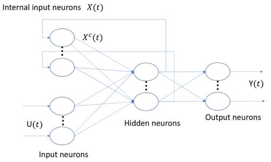
Also known as simple recurrent networks (SRN) [13]. An Elman recurrent neural networks is a two-layer backpropagation network, with feedback from the output of the hidden layer to the input of the network (Figure 1), which allows the network to detect time-varying patterns. The feedback contains a delay, allowing the network to retain values from the previous step for use in the current step, thus allowing the network to learn nonlinear patterns and predict their behavior. Equations (2) and (3) describe the basic operation of the Elman network [13,27,35].
 where
where
Figure 1.
Elman recurrent network base diagram [36].
- : input vector.
- : hidden layer vector.
- : output vector.
- W, U and b: parameter matrices and vector.
- and : activation functions.
Elman networks with feedback can learn to recognize chaotic behaviors more quickly than a simple neural network, but at the cost of increased processing time [35]. Despite increasing the time required, it is smaller in comparison to that required by other recurrent networks. Widely used in image recognition (signature recognition, element detection in photographs), a time series in which the non-linearity of the problem is a secondary factor and processing time are crucial to solving the problem [27].
3. LSTM Recurrent Neural Network
The LSTM recurrent neural network was proposed by Hochreiter and Schmidhuber (1997) [6,37]. Conventional recurrent neural networks present problems in training because backpropagated gradients tend to grow large or fade with time. After all, the gradient depends not only on the present error but also on past errors. The accumulation of errors causes difficulties in memorizing long-term dependencies [38].
These problems are solved by LSTM networks, which incorporate a series of steps to decide which information is to be stored and which is to be erased with three gates that control the way information flows in and out of the unit [37], as shown in Figure 2.
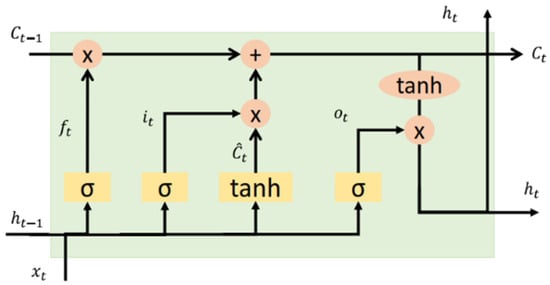
Figure 2.
Base neuron LSTM [37].
- Input gates control when new information can enter the memory.
- Forget gates control when part of the information is forgotten, allowing the cell to discriminate between important and excessive data, thus leaving room for new data.
- Output gates control when it is used as the result of the memories in the cell.
The cell has a weighting optimization mechanism based on the resulting network output error, which controls each gate. This mechanism is usually implemented with the training algorithm, BPTT. Equations (4)–(8) describe the basic functioning of LSTM neurons.
where
- : input vector.
- : forget gate activation vector.
- : input/update gate activation vector.
- W: matrix weights implemented.
- : hidden state vector, better known as the LSTM unit output vector.
4. GRU Recurrent Neural Network
The GRU recurrent neural network was introduced in 2014 by Cho et al. [10,39]. A GRU neuron is similar to the LSTM neuron but lacks an output gate, thus maintaining two gates: an update gate and a reset gate, as seen in Figure 3 [10]. The update gate indicates how much of the previous cell contents to keep, and the reset gate defines how to incorporate the new input with the earlier cell contents [16,39].
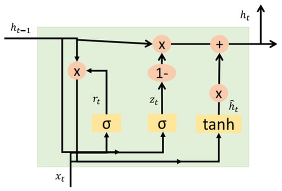
Figure 3.
Base neuron GRU [39].
Mainly used in polyphonic music modeling, speech modeling, and natural language processing, the GRU performs best on sets with a small number of data [16].
The Equations (9)–(12) describe the operation of a GRU neuron. Initializing t = 0 and the output vector = 0 [39].
where
- : input vector.
- : output vector.
- : candidate gate vector.
- : reset gate vector.
- : update gate vector.
- W, U, and b: parameter matrices and vector.Activation functions
- : sigmoid function.
- : hyperbolic tangent.
5. Case Study
In this section, the geographical area studied, characteristics of the database used, and the hardware characteristics for the analysis are explained.
5.1. Study Area
The study area corresponded to Mexico City and its surroundings (Mexico), where the RAMA network is located. Figure 4 shows the location of the monitoring stations [40,41]. The stations whose records are analyzed in this work, which are: TLA, MER, and XAL, belonging to the delegations of Tlalnepantla de Baz (State of Mexico), Venustiano Carranza (CDMX), and Ecatepec de Morelos (Mexico State), respectively [40], are highlighted in red.
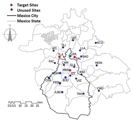
Figure 4.
Map of the distribution of stations belonging to RAMA [41].
5.2. PM Data
RAMA allows free access to its online database, which contains records of different pollutants since 1986 to date. At present, RAMA has 24 monitoring stations whose records have the following characteristics: they are daily records measured at a frequency of one hour with positive numerical values and records of atypical data denoted with a −99, which indicates that the sensor did not perform its correct operation for some external reason (malfunction, maintenance, etc.) [41]. In this study, the records in the interval from 2005 to 2019 of the particulate matter and were processed, which means that 131,472 data points were processed per monitoring station.
The behavior of PM is highly nonlinear, as shown in Figure 5, which shows the behavior of and for the first 16 days of January, 2019. Both records have a discontinuous interval, which represents no accurate record at that precise moment, and the missing values had to be proposed and interpolated to maintain continuity (section highlighted in orange).
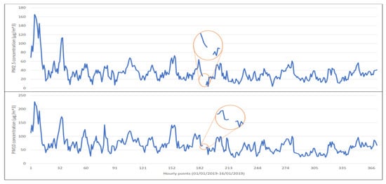
Figure 5.
Behavior recorded during the first days of January 2019 by the MER environmental station.
5.3. Hardware and Software Used
The present work was performed on a personal computer with 6 GB RAM, an NVIDIA GEFORCE GTX graphics card, and an Intel CORE I7 7th Gen processor, using PYTHON 3.6 software in conjunction with the KERAS library for deep networks.
6. Proposed Methods
The following steps were performed for the implementation of the three different deep networks, using the methodology shown in Figure 6.
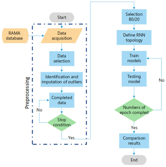
Figure 6.
Implemented methodology.
6.1. Preprocessing Data
Initially, the stations with the least amount of outlier data (measurement losses, disconnection due to maintenance, failures in the complete system, etc. [41]) were identified for both in the and records, so that the different recurrent neural network architectures evaluated only the enormous amount of data representing the actual behavior of particulate matter. Table 2 shows the stations with the smallest percentages of outlier data between 2005 to 2019, which were located in the Venustiano Carranza (MER) and Tlalnepantla de Baz (TLA) delegations, being a commercial zone and an industrial zone, with 131,472 records existing from each station, respectively [40].
Table 2.
Percentages of outliers.
The next step was to replace these records with approximate values to have continuity in the data. For this purpose, the multiple imputation by chained equations (MICE) algorithm was implemented to identify the values before and after the outliers.
MICE makes a correlation between the valid data, performing an iterative series of predictive models. Each variable specified in the data set was imputed in each iteration using the other variables in the data set. In other words, the basic idea is to treat each variable with missing values as the dependent variable in a regression, with some or all of the remaining variables as predictors. This technique uses a procedure called predictive mean matching (PMM) to generate random draws from the predictive distributions determined by the fitted models. These lucky draws become the imputed values while maintaining behavior similar to the valid data [42].
6.2. Construction Model
The three RNNs were evaluated with the same hyperparameter, architecture, training data, and validation conditions. The architecture assessed consisted of three layers, an input layer, a hidden layer, and an output layer, which are described below [6]. Each neuron of the three different layers was configured depending on the evaluated network type, which varied among Elman, GRU, and LSTM networks.
- Input layer: 50 neurons.
- Hidden layer: 250 neurons.
- Output Layer: 1 neuron.
In Table 3, the number of hyperparameters to vary during each test are listed. This generated a total of 16 individual runs, which were each repeated ten times to determine the variability of the results obtained for both the and particle sizes.
Table 3.
Hiperparameters used in this contribution.
Hyperparameters refer to the following features:
- Bach size. Defines the number of samples with which the network will work before modifying its internal parameters. Since the data are continuous records in a time series, it is necessary to divide them into sections. The network can recognize sections of the behavior using a smaller amount of memory than would be required to process all the records in a single iteration [43]. Another point of interest is the execution time, which with a small batch size tends to increase [44]. It is important to find a balance point between the execution time and the memory used; in other words, with a small batch size, the execution time increases but the error obtained is lower when working with a large batch size and consequently a shorter execution time. The batch size to be used depends on the amount of data used during the training of the network, so that the network recognizes sections continuously and is able to model the continuous behavior to predict a future behavior [43,44,45]. Essentially, the batch size allows the network to divide the problem into sections whose output variables are compared with the expected variables, obtaining an error. From this error, the network is updated and the model is improved [46]. Most of the values used corresponded to the parameter of , as shown in the literature [18]. In contrast, 96 corresponds to the multiple of 12 h represented for the prediction of exceedances exposed in [6,10].
- Optimizer. Methods by which the algorithms are used to readjust their internal parameters, thus improving the learning of the implemented algorithm. For the present work, we used the optimizers Adam and Adamax, which are widely used with time series data, because they employ a stochastic gradient method based on the adaptive estimation of first and second-order moments [15,31,47].
- Number of epochs. Defines the number of times the algorithm will use the entire training data set. During each epoch, each data sample will have the opportunity to update the internal parameters of the network [31,44], in this case, 12 epochs were used, since by using a more significant number of epochs, the network evaluation error remains practically constant with only an occasional, slight variation [6].
6.3. Model Evaluation
With its purpose of evaluating the robustness of an algorithm applied in a system with numerous variables that can affect or generate perturbations in the input parameters, the total sensitivity model evaluation method was used. Todorov et al. evaluated different stochastic approaches to evaluate the sensitivity indexes, allowing a comparison to be made between the input parameters with respect to their influence on the points of interest [48]. To evaluate the results of the time series analysis we used the root mean square error (RMSE) [49] and the correlation coefficient (CC) [50]. The variable “M” represents the values of the records modeled by the recurrent networks (Elman, LSTM, and GRU), the variable “R” is the actual records, and “n” the number of total data.
RMSE represents the difference between the data generated by the network and the actual data [49].
CC generates values between −1 and 1, being the closest to one in a positive way means that the predicted values (M) are closer to the real values (R). In other words, if the CC is equal to 1, there is no difference between the modeled data and the real data, while if a negative value is obtained it means that a mirror behavior to the real data was obtained [50]. Equation (14) shows the sections corresponding to the calculation.
where:
7. Results and Discussion
Comparison between the behavior of the real data (solid blue line) and the neural network model (solid orange line) for both and is shown in Figure 7. This comparison was made using an LSTM neural network in 2019.
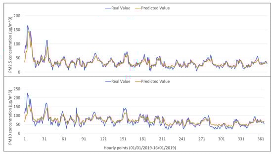
Figure 7.
Behavioral comparison of real data and data modeled by the LSTM network.
Furthermore, Figure 8 and Figure 9 shows the repeatability and the range corresponding to the CC, obtained with different batch sizes (96,128,256, and 512) and optimizers (Adam and Adamax), using the three network architectures evaluated for the behavior of the and particulate material, respectively.
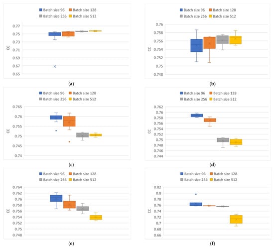
Figure 8.
CC variability obtained from modeling particle. (a) Elman neural network using Adam optimizer. (b) Elman neural network using Adamax optimizer. (c) GRU neural network using Adam optimizer. (d) GRU neural network using Adamax optimizer. (e) LSTM neural network using Adam optimizer. (f) LSTM neural network using Adamax optimizer.
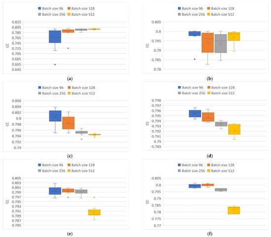
Figure 9.
CC variability in particle behavior modeling. (a) Elman neural network using Adam optimizer. (b) Elman neural network using Adamax optimizer. (c) GRU neural network using Adam optimizer. (d) GRU neural network using Adamax optimizer. (e) LSTM neural network using Adam optimizer. (f) LSTM neural network using Adamax optimizer.
Figure 8 shows the variability of the CC when using the Adam optimizer (on the right) and the Adamax optimizer (on the left) in particle modeling using the three network architectures. Figure 8a,b correspond to the results of the Elman network architecture, where the best results shown were using the Adamax optimizer, especially using a batch size of 512, with an average CC of 0.757. In contrast, with the use of the Adam optimizer for a batch size of 96, atypical data were generated, demonstrating that the network had problems in cases where the behavior of the data was highly chaotic and that for this neural network, it is better to use the Adamax optimizer.
In the case of the use of the GRU (Figure 8c,d) and LSTM (Figure 8e,f) networks, it was observed that the behavior was very similar; batch sizes of 96 obtained the best results, regardless of the optimizer used. Highlighting the following differences, in the use of the GRU network, errors were observed when the batch sizes were greater than 256, regardless of the optimizer implemented. The high repeatability obtained by the Adamax optimizer is notable. In the case of the LSTM network in conjunction with the Adamax optimizer, for tests with batch sizes of 128 and 256, it was observed that the results obtained are consistent while maintaining high repeatability with values of approximately 0.76, compared to those obtained with the use of the Adamax optimizer.
Figure 9 shows the results obtained from the CC of the particle modeling. The implemented Elman architecture (Figure 9a,b) presented the least variation in the results obtained with a batch size of 512 and the Adam optimizer, with a mean of 0.79. Curiously, highest variation occurred when the Elman architecture was presented with the batch size of 96. With the Adamax optimizer, there was a greater variation with batch sizes of 128 and 256. The best results came from the batch size of 96, followed by the batch size of 512 with approximate means of 0.799 and 0.797, respectively. For Figure 9c,d, corresponding to the GRU architecture, there was a decrease in the CC with an increase to the implemented batch size, regardless of the optimizer, as is highlighted in the greater compactness of the results with batch sizes of 256 and 512 with the Adam optimizer, with mean CC values of 0.795 and 0.794, respectively. In the case of the results with the Adamax optimizer a constant reduction was shown as the batch size increased, maintaining a practically constant amplitude of 0.002. Finally, items Figure 9e,f, corresponding to the LSTM architecture, show that with batch sizes of 96, 128, and 256, they had average CC values of 0.79 for both optimizers, with greater compactness observed with the Adam optimizer, while for a batch size of 512 there was a considerable difference. In the LSTM architecture, the optimizer does not show a representative change for this application.
In Figure 10 and Figure 11, the variability obtained from the RMSE is shown. These Figures show greater variability in the results obtained compared to those obtained from the correlation coefficient. In Figure 8a and Figure 10a, it is observed that, for the Elman network, there was an outlier point when using the Adam optimizer and a batch size of 96, indicating that when the Elman network was modeling the behavior of many of the results were below the expected performance. Conversely, with the rest of the batch sizes evaluated, high repeatability of approximately 9.9 was maintained with a 512 batch size, showing the best possible results for this topology.
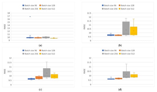
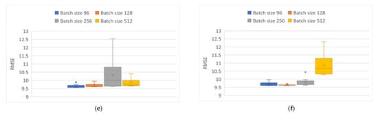
Figure 10.
RMSE variability obtained from modeling particles. (a) Elman neural network using Adam optimizer. (b) Elman neural network using Adamax optimizer. (c) GRU neural network using Adam optimizer. (d) GRU neural network using Adamax optimizer. (e) LSTM neural network using Adam optimizer. (f) LSTM neural network using Adamax optimizer.
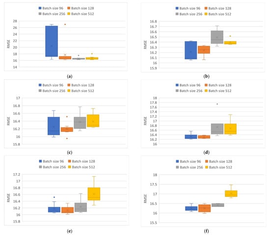
Figure 11.
RMSE variability obtained from modeling particles. (a) Elman neural network using Adam optimizer. (b) Elman neural network using Adamax optimizer. (c) GRU neural network using Adam optimizer. (d) GRU neural network using Adamax optimizer. (e) LSTM neural network using Adam optimizer. (f) LSTM neural network using Adamax optimizer.
Regarding the Adamax optimizer (Figure 10b and Figure 11b) with batch sizes of 256 and 512 there was greater variability in the results obtained, and an average of 10.25 was maintained in both cases. With batch sizes set to 96 and 128, a similar consistency was observed, with a mean of approximately 9.6. In Figure 10c,d and Figure 11c,d, corresponding to the GRU architecture, the results present a higher variability, which is more visible with batch sizes of 256 and 512 for both optimizers. With batch sizes of 96 and 128, the Adamax optimizer showed higher repeatability in the results than the Adam optimizer. Finally, Figure 10e,f and Figure 11e,f correspond to the implementation of the LSTM topology. This network presented different behavior between them; in the case of the application of the Adam optimizer there was a greater variation in the results with batch size of 256, with an average of 10.4, but this variation decreased with batch size of 512, obtaining an average of 9.9.
In contrast, with batch sizes of 128 and 96, LTSM topology presented a similar behavior. In the case of the Adamax optimizer, a more significant variation is found with a batch size of 512 and an approximate mean of 10.7 was obtained. For batch sizes of 256 and 96, similar results were obtained, highlighting an outlier for batch size of 256, with a standard for both of them of 9.6. Finally, the 128 batch size showed a low variability of the results obtained after the ten tests performed.
Figure 11a,b corresponds to the results of the Elman network implementation, which produced a wide variety of possible results with the application of the Adam optimizer with batch sizes of 96, while larger batch sizes showed higher repeatability and lower variance. However, for all three cases, outliers are shown which seem larger than the general average. Despite the high repetitiveness of the results, the Elman network seemed to have complications modeling the behavior of the particulate matter using the Adam optimizer, in the sense that the variance was higher. In the case of the Adamax optimizer implementation, the results show a comparative improvement, with high repetitiveness in the 512 batch size, with a mean of 16.6. In the case of smaller batch sizes, the mean improved as the batch size was reduced, albeit with higher variability.
In Figure 11c,d the GRU network showed different behavior for each optimizer, in which the optimizer Adam and the batch sizes of 96, 256, and 512 presented a variation in their results of 0.6 in the RMSE. For the case of the batch size of 128, there was greater repeatability of the results, but with two outliers, one at each side of the boxplot. Using the Adamax optimizer for batch sizes of 96 and 128, there was a variation in the results of 0.2 with a mean of 16.3, in contrast to the variation present with higher batch sizes.
Finally, Figure 11e,f indicate that, in the LSTM network, the expected results was observed. This means that the RMSE increased with larger batch sizes. Also, there is a difference between using the Adam and the Adamax optimizers, especially in the results of the batch size of 96. The Adam optimizer obtained results with a mean of 16.1, with a single outlier. In the case of the batch size of 128, the same low variance was observed, but without the outlier. With the Adamax optimizer, the results with greater repetitiveness were presented with the batch size of 256, for the batch size of 128 it had a mean of 16.25 with a variance of 0.5, which was greater than that present in the batch size of 96 maintaining a similar mean.
Finally, Figure 12 and Figure 13 show the behaviors of the execution times of each of the tests in the modeling of and particulate matter, respectively. In both Figures, the same behavior is observed regardless of the optimizer implemented. In other words, the execution time was higher as the batch size decreased. This was especially so with a batch size of 96, regardless of the topology implemented. However, the execution times in the modeling of the particles were higher with the Adamax optimizer, with the slowest execution being that of the LSTM network, followed by the GRU network. The Elman network was the fastest.
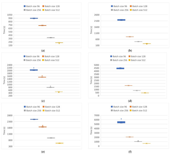
Figure 12.
Processing time variability in modeling particle behavior . (a) Elman neural network using Adam optimizer. (b) Elman neural network using Adamax optimizer. (c) GRU neural network using Adam optimizer. (d) GRU neural network using Adamax optimizer. (e) LSTM neural network using Adam optimizer. (f) LSTM neural network using Adamax optimizer.
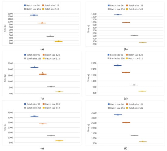
Figure 13.
Processing time variability in modeling particle behavior . (a) Elman neural network using Adam optimizer. (b) Elman neural network using Adamax optimizer. (c) GRU neural network using Adam optimizer. (d) GRU neural network using Adamax optimizer. (e) LSTM neural network using Adam optimizer. (f) LSTM neural network using Adamax optimizer.
For the particle modeling, Figure 13 indicates that the behavior recorded was practically the same, regardless of the optimizer implemented. This is also consistent with previous results in which the Elman network was the fastest topology, followed by the GRU network and the LSTM network.
Summarizing the above, Table 4 and Table 5 show the best combination of hyperparameters for each network in the modeling of and particles, respectively, indicating the average of the corresponding metrics obtained.
Table 4.
Best hyperparameters for particle modeling.
Table 5.
Best hyperparameters for PM10 particle modeling.
8. Conclusions
Evaluating three different recurrent topologies implementing a similar base architecture for and particle modeling it was observed that factors such as the optimizer used affect the results obtained. Yhe Adam optimizer showed the best results in general. At the same time, it showed greater variability in particular instances when implemented in an Elman network, in contrast with the Adamax optimizer, which maintained a lower variability in the results obtained, only having the problem of the execution time, which for a batch size of 96 was close to double that of the Adam optimizer. Mentioning the batch size, it was observed that the best results in terms of repeatability were those obtained with a batch size of 256, and in terms of the final results, comparing the CC and RMSE shows that the appropriate batch size was 128, both producing the mean values in this set of tests. The evaluated recurrent networks present great capacity for modeling the behavior of nonlinear elements such as particulate matter. Through the CC, it was determined that there was no over-training, the evaluated records from different stations maintaining repeatability in the results demonstrates the robustness of the topologies presented. Furthermore, execution times are an important factor to consider. Producing similar results obtained with different execution times, helps one determine which RNN structure is appropriate for a defined task. Considering the RMSE and CC results together with the execution time, the best network topology implemented overall used GRU neurons, but if fast results are required, the Elman network showed a higher processing capacity in a reduced time. Its only drawback is the existence of problems in in determining chaotic patterns, which must be investigated further, but if there is a large quantity of data and the execution time is not an issue to be tackled, the LSTM network is a great option for maintaining a low variability and high repeatability in the results obtained.
Author Contributions
Data curation, J.C.P.-O. and A.S.-O.; Formal analysis, M.A.A.-F. and E.G.-H.; Methodology, J.A.R.-M.; Project administration, M.A.A.-F.; Software, A.S.-O.; Validation, E.G.-H.; Visualization, J.C.P.-O.; Writing—original draft, J.A.R.-M. and M.A.A.-F.; Writing—review & editing, M.A.A.-F. All authors have read and agreed to the published version of the manuscript.
Funding
This research received no external funding.
Informed Consent Statement
Not applicable.
Data Availability Statement
Raw data is publicly available at: http://www.aire.cdmx.gob.mx/ (accessed on 15 August 2021).
Conflicts of Interest
The authors declare no conflict of interest.
References
- Brunekreef, B.; Holgate, S.T. Air pollution and health. Lancet 2002, 360, 1233–1242. [Google Scholar] [CrossRef]
- Kampa, M.; Castanas, E. Human health effects of air pollution. Environ. Pollut. 2008, 151, 362–367. [Google Scholar] [CrossRef] [PubMed]
- Sotomayor-Olmedo, A.; Aceves-Fernández, M.A.; Gorrostieta-Hurtado, E.; Pedraza-Ortega, C.; Ramos-Arreguín, J.M.; Vargas-Soto, J.E. Forecast urban air pollution in Mexico City by using support vector machines: A kernel performance approach. Int. J. Intell. Sci. 2013, 3, 10. [Google Scholar] [CrossRef] [Green Version]
- Davidson, C.I.; Phalen, R.F.; Solomon, P.A.; Davidson, C.I.; Phalen, R.F.; Airborne, P.A.S.; Davidson, C.I.; Phalen, R.F.; Solomon, P.A. Airborne Particulate Matter and Human Health: A Review. Aerosol Science and Technology. Aerosol Sci. Technol. 2005, 8, 737–749. [Google Scholar] [CrossRef]
- Aceves-Fernandez, M.A.; Pedraza-Ortega, J.C.; Sotomayor-Olmedo, A.; Ramos-Arreguín, J.M.; Vargas-Soto, J.E.; Tovar-Arriaga, S. Analysis of key features of non-linear behaviour using recurrence quantification. Case study: Urban Airborne pollution at Mexico City. Environ. Modeling Assess. 2014, 19, 139–152. [Google Scholar]
- Montañez, J.A.R.; Fernandez, M.A.A.; Arriaga, S.T.; Arreguin, J.M.R.; Calderon, G.A.S. evaluation of a recurrent neural network LSTM for the detection of exceedances of particles PM10. In Proceedings of the 2019 16th International Conference on Electrical Engineering, Computing Science and Automatic Control (CCE), Mexico City, Mexico, 11–13 September 2019; IEEE: New York, NY, USA, 2019; pp. 1–6. [Google Scholar]
- An, Z.; Jin, Y.; Li, J.; Li, W.; Wu, W. Impact of particulate air pollution on cardiovascular health. Curr. Allergy Asthma Rep. 2018, 18, 1–7. [Google Scholar] [CrossRef] [PubMed]
- Aceves-Fernández, M.A.; Domínguez-Guevara, R.; Pedraza-Ortega, J.C.; Vargas-Soto, J.E. Evaluation of Key Parameters Using Deep Convolutional Neural Networks for Airborne Pollution (PM10) Prediction. Discret. Dyn. Nat. Soc. 2020, 2020, 2792481. [Google Scholar] [CrossRef] [Green Version]
- Del Carmen Cabrera-Hernandez, M.; Aceves-Fernandez, M.A.; Ramos-Arreguin, J.M.; Vargas-Soto, J.E.; Gorrostieta-Hurtado, E. Parameters influencing the optimization process in airborne particles PM10 Using a Neuro-Fuzzy Algorithm Optimized with Bacteria Foraging (BFOA). Int. J. Intell. Sci. 2019, 9, 67–91. [Google Scholar] [CrossRef] [Green Version]
- Becerra-Rico, J.; Aceves-Fernández, M.A.; Esquivel-Escalante, K.; Pedraza-Ortega, J.C. Air-borne particle pollution predictive model using Gated Recurrent Unit (GRU) deep neural networks. Earth Sci. Inform. 2020, 13, 821–834. [Google Scholar] [CrossRef]
- Laurent, T.; von Brecht, J. A recurrent neural network without chaos. arXiv 2016, arXiv:1612.06212. [Google Scholar]
- Hua, Y.; Zhao, Z.; Li, R.; Chen, X.; Liu, Z.; Zhang, H. Deep learning with long short-term memory for time series prediction. IEEE Commun. Mag. 2019, 57, 114–119. [Google Scholar] [CrossRef] [Green Version]
- Krichene, E.; Masmoudi, Y.; Alimi, A.M.; Abraham, A.; Chabchoub, H. Forecasting using Elman recurrent neural network. In Proceedings of the International Conference on Intelligent Systems Design and Applications, Porto, Portugal, 14–16 December 2016; Springer: Berlin/Heidelberg, Germany, 2016; pp. 488–497. [Google Scholar]
- Hermans, M.; Schrauwen, B. Training and analysing deep recurrent neural networks. Adv. Neural Inf. Process. Syst. 2013, 26, 190–198. [Google Scholar]
- Fawaz, H.I.; Forestier, G.; Weber, J.; Idoumghar, L.; Muller, P.A. Deep learning for time series classification: A review. Data Min. Knowl. Discov. 2019, 33, 917–963. [Google Scholar] [CrossRef] [Green Version]
- Dey, R.; Salem, F.M. Gate-variants of gated recurrent unit (GRU) neural networks. In Proceedings of the 2017 IEEE 60th International Midwest Symposium on Circuits and Systems (MWSCAS), Boston, MA, USA, 6–9 August 2017; IEEE: New York, NY, USA, 2017; pp. 1597–1600. [Google Scholar]
- Fan, J.; Li, Q.; Hou, J.; Feng, X.; Karimian, H.; Lin, S. A spatiotemporal prediction framework for air pollution based on deep RNN. In Proceedings of the ISPRS Annals of the Photogrammetry, Remote Sensing and Spatial Information Sciences 2017, Cambridge, MA, USA, 7–9 August 2017; Volume 4, p. 15. [Google Scholar]
- Rojas, R. Neural Networks: A Systematic Introduction; Springer Science & Business Media: Berlin/Heidelberg, Germany, 2013. [Google Scholar]
- Vicente, A.B.; Juan, P.; Meseguer, S.; Díaz-Avalos, C.; Serra, L. Variability of PM10 in industrialized-urban areas. New coefficients to establish significant differences between sampling points. Environ. Pollut. 2018, 234, 969–978. [Google Scholar] [CrossRef] [PubMed]
- Mannucci, P.M.; Harari, S.; Martinelli, I.; Franchini, M. Effects on health of air pollution: A narrative review. Intern. Emerg. Med. 2015, 10, 657–662. [Google Scholar] [CrossRef]
- Landrigan, P.J.; Fuller, R.; Acosta, N.J.; Adeyi, O.; Arnold, R.; Baldé, A.B.; Bertollini, R.; Bose-O’Reilly, S.; Boufford, J.I.; Breysse, P.N.; et al. The Lancet Commission on pollution and health. Lancet 2018, 391, 462–512. [Google Scholar] [CrossRef] [Green Version]
- Manisalidis, I.; Stavropoulou, E.; Stavropoulos, A.; Bezirtzoglou, E. Environmental and health impacts of air pollution: A review. Front. Public Health 2020, 8, 14. [Google Scholar] [CrossRef] [PubMed] [Green Version]
- Otter, D.W.; Medina, J.R.; Kalita, J.K. A survey of the usages of deep learning for natural language processing. IEEE Trans. Neural Netw. Learn. Syst. 2020, 32, 604–624. [Google Scholar] [CrossRef] [Green Version]
- Wu, Y.; Ji, X.; Ji, W.; Tian, Y.; Zhou, H. CASR: A context-aware residual network for single-image super-resolution. Neural Comput. Appl. 2019, 32, 14533–14548. [Google Scholar] [CrossRef]
- Liu, Z.; Xu, W.; Feng, J.; Palaiahnakote, S.; Lu, T. Context-aware attention lstm network for flood prediction. In Proceedings of the 2018 24th International Conference On Pattern Recognition (ICPR), Beijing, China, 20–24 August 2018; IEEE: New York, NY, USA, 2018; pp. 1301–1306. [Google Scholar]
- Naira, T.; Alberto, C. Classification of people who suffer schizophrenia and healthy people by EEG signals using deep learning. Int. J. Adv. Comput. Sci. Appl. 2019, 10. [Google Scholar] [CrossRef]
- Hu, H.; Wang, H.; Bai, Y.; Liu, M. Determination of endometrial carcinoma with gene expression based on optimized Elman neural network. Appl. Math. Comput. 2019, 341, 204–214. [Google Scholar] [CrossRef]
- Schmidhuber, J. Deep learning in neural networks: An overview. Neural Netw. 2015, 61, 85–117. [Google Scholar] [CrossRef] [PubMed] [Green Version]
- Wang, S.C. Artificial neural network. In Interdisciplinary Computing in Java Programming; Springer: Berlin/Heidelberg, Germany, 2003; pp. 81–100. [Google Scholar]
- Song, X.; Liu, Y.; Xue, L.; Wang, J.; Zhang, J.; Wang, J.; Jiang, L.; Cheng, Z. Time-series well performance prediction based on Long Short-Term Memory (LSTM) neural network model. J. Pet. Sci. Eng. 2020, 186, 106682. [Google Scholar] [CrossRef]
- Tealab, A. Time series forecasting using artificial neural networks methodologies: A system-atic review. Future Comput. Inform. J. 2018, 3, 334–340. [Google Scholar] [CrossRef]
- Hassoun, M.H. Fundamentals of Artificial Neural Networks; MIT Press: Cambridge, MA, USA, 1995. [Google Scholar]
- Abraham, A. Handbook of measuring system design. In Artificial Neural Networks; Oklahoma State University: Stillwater, OK, USA, 2005. [Google Scholar]
- Xayasouk, T.; Lee, H.; Lee, G. Air pollution prediction using long short-term memory (LSTM) and deep autoencoder (DAE) models. Sustainability 2020, 12, 2570. [Google Scholar] [CrossRef] [Green Version]
- Chandra, R. Competition and collaboration in cooperative coevolution of Elman recurrent neural networks for time-series prediction. IEEE Trans. Neural Netw. Learn. Syst. 2015, 26, 3123–3136. [Google Scholar] [CrossRef] [Green Version]
- Übeyli, E.D.; Übeyli, M. Case studies for Applications of Elman Recurrent Neural Networks; IntechOpen: London, UK, 2008. [Google Scholar]
- Hochreiter, S.; Schmidhuber, J. Long short-term memory. Neural Comput. 1997, 9, 1735–1780. [Google Scholar] [CrossRef]
- Muzaffar, S.; Afshari, A. Short-term load forecasts using LSTM networks. Energy Procedia 2019, 158, 2922–2927. [Google Scholar] [CrossRef]
- Chung, J.; Gulcehre, C.; Cho, K.; Bengio, Y. Empirical evaluation of gated recurrent neural networks on sequence modeling. arXiv 2014, arXiv:1412.3555. [Google Scholar]
- CDMX. Bases de Datos–Red Automática de Monitoreo Atmosférico (RAMA). 2019. Available online: http://www.aire.cdmx.gob.mx/default.php?opc=%27aKBh%27 (accessed on 8 September 2019).
- Instituto Nacional de Ecología y Cambio Climático. Informe Nacional de Calidad del Aire 2018; Instituto Nacional de Ecología y Cambio Climático: Mexico City, Mexico, 2019. [Google Scholar]
- Cao, W.; Wang, D.; Li, J.; Zhou, H.; Li, L.; Li, Y. Brits: Bidirectional recurrent imputation for time series. arXiv 2018, arXiv:1805.10572. [Google Scholar]
- You, Y.; Wang, Y.; Zhang, H.; Zhang, Z.; Demmel, J.; Hsieh, C.J. The Limit of the Batch Size. arXiv 2020, arXiv:2006.08517. [Google Scholar]
- Smith, L.N. A disciplined approach to neural network hyper-parameters: Part 1–learning rate, batch size, momentum, and weight decay. arXiv 2018, arXiv:1803.09820. [Google Scholar]
- Brownlee, J. What is the Difference Between a Batch and an Epoch in a Neural Network? Mach. Learn. Mastery 2018, 20, 1–5. [Google Scholar]
- Proskuryakov, A. Intelligent system for time series forecasting. Procedia Comput. Sci. 2017, 103, 363–369. [Google Scholar] [CrossRef]
- Liu, H.; Yan, G.; Duan, Z.; Chen, C. Intelligent modeling strategies for forecasting air quality time series: A review. Appl. Soft Comput. 2021, 102, 106957. [Google Scholar] [CrossRef]
- Todorov, V.; Dimov, I.; Ostromsky, T.; Apostolov, S.; Georgieva, R.; Dimitrov, Y.; Zlatev, Z. Advanced stochastic approaches for Sobol’sensitivity indices evaluation. Neural Comput. Appl. 2021, 33, 1999–2014. [Google Scholar] [CrossRef]
- Park, J.H.; Yoo, S.J.; Kim, K.J.; Gu, Y.H.; Lee, K.H.; Son, U.H. PM10 density forecast model using long short term memory. In Proceedings of the 2017 Ninth International Conference on Ubiquitous and Future Networks (ICUFN), Milan, Italy, 4–7 July 2017; IEEE: New York, NY, USA, 2017; pp. 576–581. [Google Scholar]
- Zhu, H.; Zhu, Y.; Wu, D.; Wang, H.; Tian, L.; Mao, W.; Feng, C.; Zha, X.; Deng, G.; Chen, J.; et al. Correlation coefficient based cluster data preprocessing and LSTM prediction model for time series data in large aircraft test flights. In Proceedings of the International Conference on Smart Computing and Communication, Tokyo, Japan, 10–12 December 2018; Springer: Berlin/Heidelberg, Germany, 2018; pp. 376–385. [Google Scholar]
Publisher’s Note: MDPI stays neutral with regard to jurisdictional claims in published maps and institutional affiliations. |
© 2021 by the authors. Licensee MDPI, Basel, Switzerland. This article is an open access article distributed under the terms and conditions of the Creative Commons Attribution (CC BY) license (https://creativecommons.org/licenses/by/4.0/).