From Stress to Shape: Equilibrium of Cloister and Cross Vaults

Abstract

The assessment of the equilibrium and the safety of masonry vaults is of high relevance for the conservation and restoration of historical heritage. In the literature many approaches have been proposed for this tasks, starting from the 17th century. In this work we focus on the Membrane Equilibrium Analysis, developed under the Heyman’s theory of Limit Analysis. Within this theory, the equilibrium of a vault is assessed if it is possible to find at least one membrane surface, between the volume of the vaults, being in equilibrium under the given loads through a purely compressive stress field. The equilibrium of membranes is described by a second order partial differential equation, which is definitely elliptic only when a negative semidefinite stress is assigned, and the shape is the unknown of the problem. The proposed algorithm aims at finding membrane shapes, entirely comprised between the geometry of the vault, in equilibrium with admissible stress fields, through the minimization of an error function with respect to shape parameters of the stress potential, and then, with respect to the boundary values of the membrane shape. The application to two test cases shows the viability of this tool for the assessment of the equilibrium of existing masonry vaults.

1. Introduction

The assessment of the equilibrium of masonry structure is a topic of high relevance, given the diffuse presence of masonry buildings in Italy and Europe, often with high historical value.

Over the centuries, different methodologies have been developed for the assessment of the equilibrium of masonry constructions and to quantify their degree of safety, starting from practical rules [1], until the definition of graphical methods applied to two dimensional structures (such as portals, bridges, and flying buttresses [2,3]) and to axis-symmetric vaults under monoaxial stress regimes, such as masonry domes [4]. Graphical methods have been extended to consider also biaxial stress states, again under the hypothesis of axial symmetry of the structure [5].

For masonry material, the starting hypotheses have been clearly formulated by Heyman in [6,7], and assume that the material is infinitely resistant in compression and that sliding between rigid blocks does not occur inside the material. Under these assumptions, the theorems of Limit Analysis hold, and an equilibrium solution is defined as admissible if it is balanced with the given loads and is everywhere of pure compression. In particular, based on the Safe Theorem, the impossibility of collapse of a masonry structure, under the given loads, is ensured if at least one admissible equilibrium solution can be found.

A wide number of methods have been developed for the assessment of masonry vaults within the Heyman’s theory, both considering the kinematic and the Static Theorem. Concerning the Kinematic theorem of Limit Analysis, the proposed methods are based on energy criteria minimization. Indeed, the minimum of the total potential energy can be used to look at both stable and non-stable mechanisms [8,9]. Moreover, it can be also used to couple internal stress states with the corresponding mechanisms as in [10]. Other methods, such as the Thrust Network Analysis (TNA), are based on the application of the Static Theorem. TNA, introduced in [11] and developed in [12,13,14,15,16], consists in the discretization of a masonry vault through a finite number of compressed bars, in equilibrium with the load of the vault, and located in-between the intrados and the extrados [17].

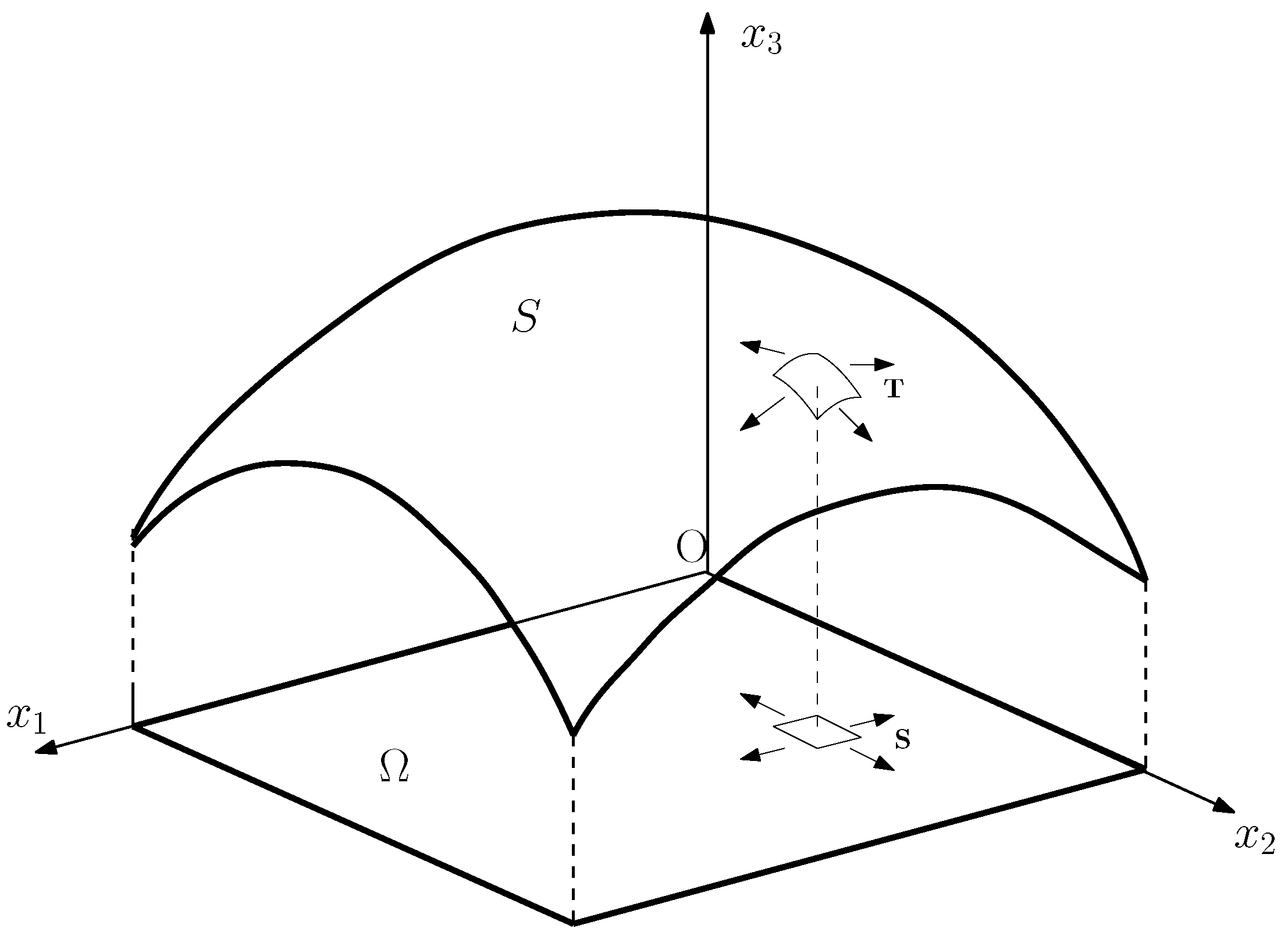
Among different continuum approach methods, here we focus on the Membrane Equilibrium Analysis (MEA), first proposed in [18], and further developed in [19]. For the assessment of the equilibrium of a vault, MEA requires to find at least one membrane surface comprised in-between the geometrical boundary of the vault, balancing the external loads through a negative semi-definite membrane stress field.

In MEA, the equilibrium is reduced to a scalar second order partial differential equation with non-constant coefficients. If the shape of the membrane is assigned, the coefficients are the components of the curvature of the membrane, and the unknown of the problem is the stress potential of the membrane stress projected onto a reference plane (Pucher stress). On the contrary, if the stress potential is assigned, the coefficients of the equation are the components of the Hessian of the stress potential and the unknown is the scalar function defining the elevation of the surface with respect to the reference plane. In both cases, the equilibrium equation may change its behaviour (hyperbolic-parabolic-elliptic) depending on the assigned shape or on the assigned stress potential. This has a strong implication on the numerical solution of the equilibrium equation, that can be solved as a boundary value problem when the equation is elliptic, or as an evolutionary problem when the equilibrium equation is hyperbolic at least in a part of the domain.

MEA has been adopted mainly for the assessment of the equilibrium of masonry constructions [20,21,22,23,24], but it is a general tool for computing the stress field on curved membrane surfaces. For example, it has been used for the evaluation of the stress field of soft tissues, such as the human cornea [25].

An approach similar to MEA, based on the search of the Airy stress function, has been proposed in [26], where NURBS are used for the discretization, exploiting their high-order continuity.

In [27] a numerical iterative procedure for the assessment of the equilibrium of masonry vaults, based on LSM (a FEM-like approximation of the governing equation, see [28]), has been introduced. Starting from a tentative membrane shape, included in the volume of the vault, the method looks for an equilibrated concave stress potential, ensuring the negative semi-definiteness of the corresponding stress. This procedure, however, is not easily applied to non-concave shapes, such as cross vaults given the non-ellipticity of the corresponding equilibrium equation. Recently, in [29] a numerical procedure based on standard FEM, for the design of purely compressed shells, has been put forward. With this method, the starting point is a class of concave stress potentials, and the equilibrium equation is purely elliptic.

In the present paper, focusing on the assessment of the equilibrium of existing masonry vaults, we start from a family of concave stress potentials in order to ensure the admissibility of the stress field. This implies the ellipticity of the equilibrium equation: Therefore, we look for an optimal membrane shape comprised between the geometrical boundary of the vault, as required by the Safe Theorem of Limit Analysis. We approach this problem through an optimization algorithm, minimizing an error function first with respect to the parameters of the stress potential, and then with respect to the boundary conditions of the the membrane shape.

Optimization is a recurring tool in different engineering applications. In the present work, we find an optimal ideal membrane shape, which best satisfies the requirements of the Safe Theorem of Limit Analysis, which result in some mathematical constraints. We point out that this is not the case of a shape optimization, since the shape of the analyzed vaults is fixed, and we just optimize an ideal membrane. In other engineering application, however, the shape of structures is optimized under the constraints of material saving, or compliance minimization. This is the case of the Structural Topology Optimization [30], used for optimally distribute the material to minimize the compliance o structures under given loads [31,32,33]. Optimization is also used in geotechnical applications [34], optimization of geodesic domes [35], of soil-steel structures [36], and lightweight structure [37]

2. Mathematical Preliminaries

In this section some mathematical details concerning the formulation of the equilibrium equation of a membrane are recalled, the notation is introduced, and the unilateral constraints on the material are introduced.

2.1. Geometry and Equilibrium

Referring to Figure 1 for notation, the geometry of a generic membrane surface S contained inside a typical shell structure can be described in Monge form in terms of the position vector $\mathbf{x}$ of the points of S as follows:

$$\mathbf{x}=x_1{\mathbf{e}}_1+x_2{\mathbf{e}}_2+f{\mathbf{e}}_3$$

(1)

where $\{{\mathbf{e}}_1,{\mathbf{e}}_2,{\mathbf{e}}_3\}$ is the orthonormal triad coherent with a given Cartesian frame $\{O;x_1,x_2,x_3\}$, the couple of coordinates $(x_1,x_2)$, which are the parameters of the curvilinear description (1), belongs to a region $\mathsf{\Omega }$ of the plane $\{O;x_1,x_2\}$ called planform of S, and $f=f(x_1,x_2)$ is the rise of the membrane with respect to the $x_1-x_2$ plane. We assume $f\in C^0\left(\mathsf{\Omega }\right)$—that is to say that the considered surface S is continuous but not necessarily smooth.

An efficient way to describe the membrane equilibrium of a membrane under a surface load $\mathbf{q}$ per unit area, is the formulation proposed by Pucher in [38]. Pucher analysis is based on the introduction of the projected stress $\mathbf{S}$, in terms of which two of the three equilibrium equations for the membrane can be made independent of the membrane shape.

The membrane stresses are tangent in each point to the membrane surface S. Therefore it is convenient to introduce a curvilinear basis on the membrane, which are computed as

$${\mathbf{a}}_{\alpha }=\frac{\partial \mathbf{x}}{\partial x^{\alpha }},\alpha =1,2$$

(2)

In addition, it is useful to introduce the contravariant basis ${\mathbf{a}}^{\alpha }$. $\alpha =1,2$ defined such that ${\mathbf{a}}_{\alpha }·{\mathbf{a}}_{\beta }={\delta }_{\alpha }^{\beta }$, being ${\delta }_{\alpha }^{\beta }$ the Kronecker delta.

Therefore we can decompose the membrane generalized stress tensor as

$$\mathbf{T}=T^{\alpha \beta }{\mathbf{a}}_{\alpha }\otimes {\mathbf{a}}_{\beta },$$

(3)

where $T^{\alpha \beta }$ are the contravariant components of the generalized stress. The projected (Pucher) stress components $S_{\alpha \beta }$ (see Figure 1) are easily defined in terms of $T^{\alpha \beta }$ as $S_{\alpha \beta }=J{T}^{\alpha \beta }$, J being the ratio between the surface area and the projected area. In terms of Pucher stress components, the vector equilibrium equation, projected into the non-orthonormal vector basis ${\mathbf{e}}_1,{\mathbf{e}}_2,\mathbf{n}={\mathbf{a}}_3$, $\mathbf{n}$ being the unit normal to S, becomes:

$$S_{11,1}+S_{12,2}+p_1=0,S_{21,1}+S_{22,2}+p_2=0,S_{\alpha \beta }f{,}_{\alpha \beta }-p_{\gamma }f{,}_{\gamma }+p_3=0.$$

(4)

where $\{p_1,p_2,p_3\}$ are the Cartesian components in the given reference of $\mathbf{p}=J\mathbf{q}$, that is the load per unit projected area. By using the projected stress, the first two equilibrium equations do not depend on the membrane shape and are the same as for the plane stress problem. In the case of pure vertical loading, say $\mathbf{p}=p{\mathbf{e}}_3$, the first two equations can be solved introducing an Airy stress potential $F(x_1,x_2)$—that here we only assume to be continuous—defined such that

$$S_{11}=F{,}_{22},S_{22}=F{,}_{11},S_{12}=S_{12}=-F{,}_{12}.$$

(5)

The third equation of (4) expresses the balance of the vertical component of the force $p_3=\mathbf{p}·{\mathbf{e}}_3$ with the scalar product between the Pucher stress tensor and the Hessian of the function f, that defines the curvature of the surface. On introducing (5) into (4), we obtiain, as transversal equilibrium equation

$$F{,}_{11}f{,}_{22}+F{,}_{22}f{,}_{11}-2F{,}_{12}f{,}_{12}+p_3=0$$

(6)

Equation (6) is a second order partial differential equation, that can be either elliptic, parabolic or hyperbolic, depending on its (usually non-constant) coefficients. If the problem is hyperbolic or parabolic, the characteristic lines are real and the problem must be formulated as an evolutionary problems by assigning two scalar conditions on a non-characteristic line.

If Equation (6) is elliptic, the problem can be formulated as a boundary value problem and the boundary conditions for this equation can be either of the Dirichlet type, i.e.,

$${F|}_{\partial \mathsf{\Omega }}=p$$

(7)

or Neumann type, i.e.,

$$\frac{\partial F}{\partial n}{|}_{\partial \mathsf{\Omega }}=q$$

(8)

where p and q are known function on the boundary $\partial \mathsf{\Omega }$, and $\mathbf{n}$ is the outward unit vector normal to the boundary.

The advantage of boundary value problems is that the solution of the corresponding discretized partial differential equation can be obtained by a simple matrix inversion.

2.2. Unilateral Constrains and Singular Stresses

The restrictions that the generalized stress $\mathbf{T}$ is negative semi-definite and does not work for the corresponding strain $\mathbf{E}$, that is positive semi-definite, define Rigid No-Tension (RNT) materials in the sense of Heyman. In formulae:

$$\mathbf{T}\in Sy{m}^{-},\mathbf{E}\in Sy{m}^{+},\mathbf{T}·\mathbf{E}=0.$$

(9)

The first application of Pucher’s transformation for NT masonry vaults can be found in [18], where it is shown that, due to the NT constraint, both the surface generalized stress and the matrix of the projected stresses must be negative semi-definite. In terms of the stress function F, this condition can be written as

$$F{,}_{11}+F{,}_{22}\le 0,F{,}_{11}F{,}_{22}-F{,}_{12}^2\ge 0.$$

(10)

The condition of semi-definiteness of the stress correspond to concavity of the stress potential.

3. Outline of the Method

The Membrane Equilibrium Analysis (MEA) applied to masonry vaults, requires to find a membrane surface located in between the intrados and the extrados of the vault and, according to Heyman’s assumptions, sustaining the loads through compressive stresses. The membrane is a determined structure, and this last constraint is generally not satisfied on a given membrane shape for given loads. In such a case, the membrane shape has to be changed iteratively from an initial guess shape, until one that satisfies the unilateral restrictions on the stress is found.

3.1. Unknowns and Data in the Governing Equilibrium Equation

On adopting a numerical discretization method based on a variational approximation of the governing Equation (6), such as the Finite Element Method, or the Lumped Stress Method defined below, the differential equation must be elliptic. Therefore, if the unknown is the stress and the given form of the membrane is not everywhere convex or concave, these methods of approximation fail and cannot be applied. A possible way out, already proposed in [29], consists in switching the roles of unknowns and data, by assuming a parametric family of concave stress potentials as given, and considering the shape as the unknown. Then, the equation is elliptic for any choice of the parameters defining a specific member of the given family of stress potentials, and the corresponding shape can be obtained by prescribing convenient boundary data for the shape. Besides, for any such concave stress potential, there exists a small repertoire of purely compressed equilibrium shapes, that one can also explore, depending on the possibly different boundary data, that can be imposed on the shape. In the present paper, the equilibrium solution is tackled by constructing an LSM approximation of the fundamental second order differential equation of equilibrium (6). This computer routine, which returns a shape associated to any given stress function, can be manipulated by changing, following a minimization algorithm, the parameters controlling the stress potential and the boundary data for the shape.

3.2. Numerical Discretization and Algorithm

The transverse equilibrium Equation (6) is solved numerically by discretizing the domain into a finite number of triangular elements, and adopting a Lumped Stress Method [28] approximation of the Hessian of both the stress potential F and of the membrane shape f. With the LSM approximation, the two functions are described by simplicial surfaces, defined by the nodal values ${\widehat{F}}_i$ and ${\widehat{f}}_i$, with $i=1,2,\dots ,N$, N being the total number of nodes of the given triangulation.

The vectors collecting the nodal values of the shape function f and of the stress potential F are denoted $\widehat{\mathbf{f}}$ and $\widehat{\mathbf{F}}$. $\widehat{\mathbf{f}}$ is divided into two vectors ${\widehat{\mathbf{f}}}_I$ and ${\widehat{\mathbf{f}}}_B$, of length $N_I$ and $N_B$, distinguishing between internal and boundary nodes, respectively.

The search of a statically admissible stress regime for the vault is carried out through an algorithm divided in several steps. Given the geometry of the vault, defined by its intrados and extrados, we start on assigning an appropriate functional form for the stress potential, depending on a limited number n of parameters, such that

$$F=F(x_1,x_2;a_1,a_2,\dots ,a_n).$$

(11)

A first step is the parametric solution of the discretized version of Equation (6), with suitable boundary conditions, in terms of the membrane shape defined by f; therefore, $f=f(x_1,x_2;a_1,a_2,\dots ,a_n)$.

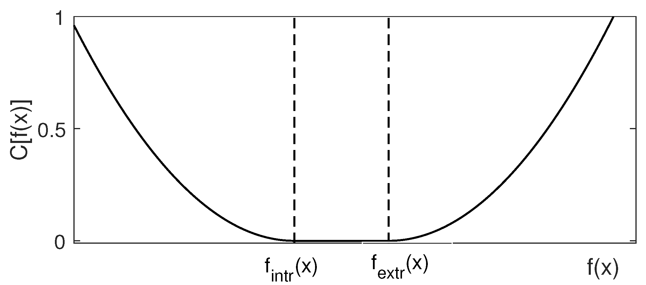
The second step consists in the optimization of the parameters $a_1,a_2,\dots ,a_n$, performed by minimizing an error function I defined as the integral of the quadratic approximation of the characteristic function of the vault domain.

Given a point $\mathbf{x}\in \mathsf{\Omega }$, the characteristic function indicates whether the corresponding values of the rise of the membrane is comprised between the volume of the vault, or not. In particular

$$C\left(f\left(\mathbf{x}\right)\right)=\left\{\begin{array}{c}\begin{array}{cc}0\hfill & \mathrm{if}{f}_{intr}\left(\mathbf{x}\right)<f\left(\mathbf{x}\right)<f_{extr}\left(\mathbf{x}\right)\hfill \\ +\infty \hfill & \mathrm{if}f\left(\mathbf{x}\right)<f_{intr}\left(\mathbf{x}\right)\mathrm{or}f\left(\mathbf{x}\right)>f_{extr}\left(\mathbf{x}\right)\hfill \end{array}\hfill \end{array}\right..$$

(12)

Its quadratic approximation reads

$$C\left(f\left(\mathbf{x}\right)\right)=\left\{\begin{array}{c}\begin{array}{cc}0\hfill & f_{intr}\left(\mathbf{x}\right)<f\left(\mathbf{x}\right)<f_{extr}\left(\mathbf{x}\right)\hfill \\ {\left(f\left(\mathbf{x}\right)-f_{intr}\left(\mathbf{x}\right)\right)}^2\hfill & f\left(\mathbf{x}\right)<f_{intr}\left(\mathbf{x}\right)\hfill \\ {\left(f\left(\mathbf{x}\right)-f_{extr}\left(\mathbf{x}\right)\right)}^2\hfill & f\left(\mathbf{x}\right)>f_{extr}\left(\mathbf{x}\right)\hfill \end{array}\hfill \end{array}\right..$$

(13)

For a generic point $\mathbf{x}$ of the domain, given $f_{intr}\left(\mathbf{x}\right)$ and $f_{extr}\left(\mathbf{x}\right)$, the approximated characteristic function is represented in Figure 2.

We denote ${\mathsf{\Omega }}_c$ the subregion of the entire planform $\mathsf{\Omega }$ obtained by removing from the domain a boundary strip of size c, defined as a fraction of the diameter L of $\mathsf{\Omega }$ (in the applications we set $c=L/5$). The rationale behind this procedure is linked to the nature of the governing equation: due to ellipticity, the solution is only weakly dependent on the boundary data, that is, altering the boundary values has a detectable effect only in a narrow band close to the boundary. So, we can split the optimization into an interior and an exterior part, postponing the optimization of the boundary data.

The error function I is then defined as follows:

$$I={\int }_{\partial {\mathsf{\Omega }}_a}{(f-f_{intr})}^{2}d\mathsf{\Omega }+{\int }_{\partial {\mathsf{\Omega }}_b}{(f-f_{extr})}^{2}d\mathsf{\Omega }$$

(14)

${\mathsf{\Omega }}_a$ and ${\mathsf{\Omega }}_b$ being the parts of the domain ${\mathsf{\Omega }}_c$, for which the membrane surface is below the intrados, or above the extrados, respectively.

In the third step, the values of $a_1,a_2,\dots ,a_n$, found in the previous step, are fixed and the boundary values of the discretized membrane shape are considered as variables. Then, the discretized version of Equation (6) is solved parametrically with respect to these boundary values. In the vector notation introduced above, the transverse equilibrium equation reads

$$\left(K_{xx,Hj}{\widehat{f}}_j\right)\left(K_{yy,Hh}{\widehat{F}}_h\right)+\left(K_{yy,Hj}{\widehat{f}}_j\right)K_{xx,Hh}{\widehat{F}}_h)-2\left(K_{xy,Hj}{\widehat{f}}_j\right)\left(K_{xy,Hh}{\widehat{F}}_h\right)+{\widehat{p}}_H=0$$

(15)

where the summation convention on repeated indices is assumed on the lower-case indices $(j,h=1,2,\dots ,N)$, whilst the upper-case index $H(H=1,2,\dots ,N_I)$ is not summed, and ${\mathbf{K}}_{xx}$, ${\mathbf{K}}_{yy}$, and ${\mathbf{K}}_{xy}$ are coefficient matrices computed via the LSM scheme, representing the discrete counterparts of the second derivatives ${\partial }^2/\partial x_1^2$, ${\partial }^2/\partial x_2^2$, and ${\partial }^2/\partial x_1\partial x_2$.

Equation (15) can be rewritten in a compact form by factoring out the unknown term $\widehat{\mathbf{f}}$, as

$$K_{ij}{\widehat{f}}_j+{\widehat{p}}_i=0,$$

(16)

where

$$K_{ij}=\left(K_{yy,Hh}{\widehat{F}}_h\right)K_{xx,Hj}+(K_{xx,Hh}{\widehat{F}}_h)K_{yy,Hj}-2(K_{xy,Hh}{\widehat{F}}_h)K_{xy,Hj}.$$

(17)

Expression (16) can be also rewritten distinguishing between boundary conditions and domain equations, in the form

$${\mathbf{K}}_{II}{\widehat{\mathbf{f}}}_I+{\mathbf{K}}_{IB}{\widehat{\mathbf{f}}}_B+{\widehat{\mathbf{p}}}_I=\mathbf{0},{\widehat{\mathbf{f}}}_B={\overline{\mathbf{f}}}_B,$$

(18)

where ${\mathbf{K}}_{II}$ and ${\mathbf{K}}_{IB}$ are submatrices of $\mathbf{K}$ corresponding to rows and columns associated to internal and boundary nodes. Finally, ${\overline{\mathbf{f}}}_B$ is the vector of the boundary parameters. From Equation (18), ${\overline{\mathbf{f}}}_I$ can be evaluated as

$${\widehat{\mathbf{f}}}_I={\mathbf{K}}_{II}^{-1}({\widehat{\mathbf{p}}}_I-{\mathbf{K}}_{IB}{\overline{\mathbf{f}}}_B).$$

(19)

On introducing (19) into a discrete version $I_2$ of the objective function I, we get

$$I_2=\sum _{i=1}^{N_a}{(f_i-f_{intr,i})}^2+\sum _{i=1}^{N_b}{(f_i-f_{extr,i})}^2.$$

(20)

We then optimize $I_2\left({\widehat{\mathbf{f}}}_I\right)$ with respect to ${\overline{\mathbf{f}}}_B$.

Notice that it is possible to compute explicitly the gradient of $I_2\left(f_I\left(f_B\right)\right)$ through the chain rule, in the form

$$\frac{\partial I_2}{\partial f_{B,j}}=\frac{\partial I}{\partial f_{I,h}}\frac{\partial f_{I,h}}{\partial f_{B,j}}$$

(21)

that is

$$\frac{\partial I_2}{\partial f_{B,j}}=\left\{\begin{array}{c}\begin{array}{cc}-2f_{i,h}{\left(K_{II}{K}_{IB}\right)}_{hj}\hfill & f_i<f_{i,intr}\mathrm{or}{f}_i>f_{i,extr}\hfill \\ 0\hfill & \mathrm{otherwise}\hfill \end{array}\hfill \end{array}\right..$$

(22)

The membrane shape obtained at the end of this minimization process can be compared to the actual geometry of the vault. If the final value of the objective function $I_2$ is zero, the membrane is completely comprised between the intrados and the extrados of the considered vault, and therefore the solution is statically admissible and proves the stability of the vault under the given loads, according to the Safe Theorem of Limit Analysis. In such a case, the degree of safeness of the structure can be assessed by reducing the slenderness of the vault and computing a geometrical safety factor, as proposed by Heyman [6].

4. Application

4.1. Cloister Vault

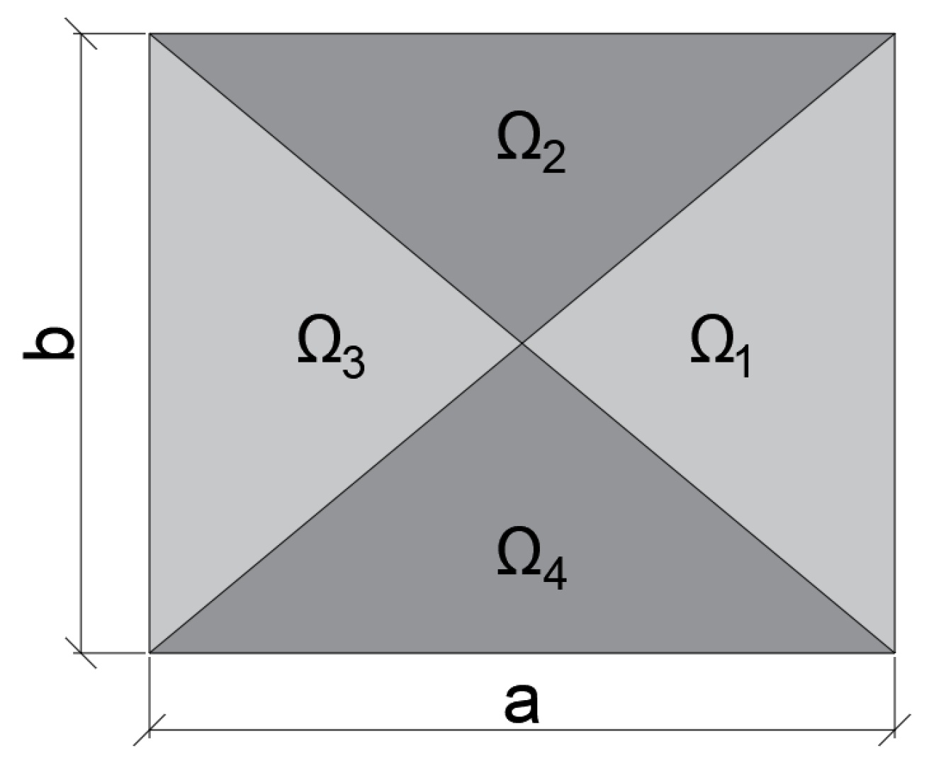
Consider the case of a cloister vault under its self-weight, whose geometry is described by the volume enclosed in-between two surfaces, the intrados and the extrados, defined canonically inside the domain $\mathsf{\Omega }=\{(x_1,x_2)\in \left[-L,L\right]\times \left[-L,L\right]\}$ as follows:

$$f_{intr}(x_1,x_2)=\left\{\begin{array}{c}\begin{array}{cc}-h{\left(\frac{x_1}{L}\right)}^2\hfill & \hfill (x_1,x_2)\in ({\mathsf{\Omega }}_1\cup {\mathsf{\Omega }}_3)\\ -h{\left(\frac{x_2}{L}\right)}^2\hfill & \hfill (x_1,x_2)\in ({\mathsf{\Omega }}_2\cup {\mathsf{\Omega }}_4)\end{array}\hfill \end{array}\right.$$

(23)

$$f_{extr}(x_1,x_2)=\left\{\begin{array}{c}\begin{array}{cc}-h{\left(\frac{x_1}{L+t}\right)}^2+t\hfill & \hfill (x_1,x_2)\in ({\mathsf{\Omega }}_1\cup {\mathsf{\Omega }}_3)\\ -h{\left(\frac{x_2}{L+t}\right)}^2+t\hfill & \hfill (x_1,x_2)\in ({\mathsf{\Omega }}_2\cup {\mathsf{\Omega }}_4)\end{array}\hfill \end{array}\right.$$

(24)

where ${\mathsf{\Omega }}_1$, ${\mathsf{\Omega }}_2$, ${\mathsf{\Omega }}_3$, and ${\mathsf{\Omega }}_4$ are the subregions of $\mathsf{\Omega }$ depicted in Figure 3.

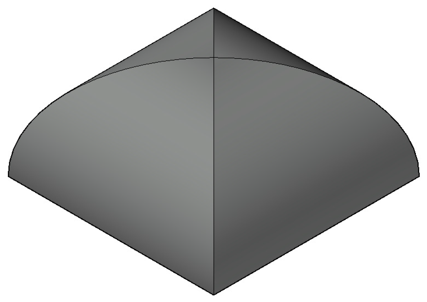
A perspective representation of the midsurface of this vault is represented in Figure 4.

The values adopted in Equations (23) and (24) are $L=2.5$ m, $h=2.13$ m, and $t=0.23$ m. The values have been taken by the geometry of the vault analyzed in [21], and located in the interior of Palazzo Caracciolo di Avellino in Naples. From [21] we also assume $p=8$ kN/m${}^2$ as distributed load per unit projected area.

By following the methodology described in Section 3, the transverse equilibrium Equation (6) can be solved for the geometry $f(x_1,x_2)$, by assuming a special parametric form for the stress potential.

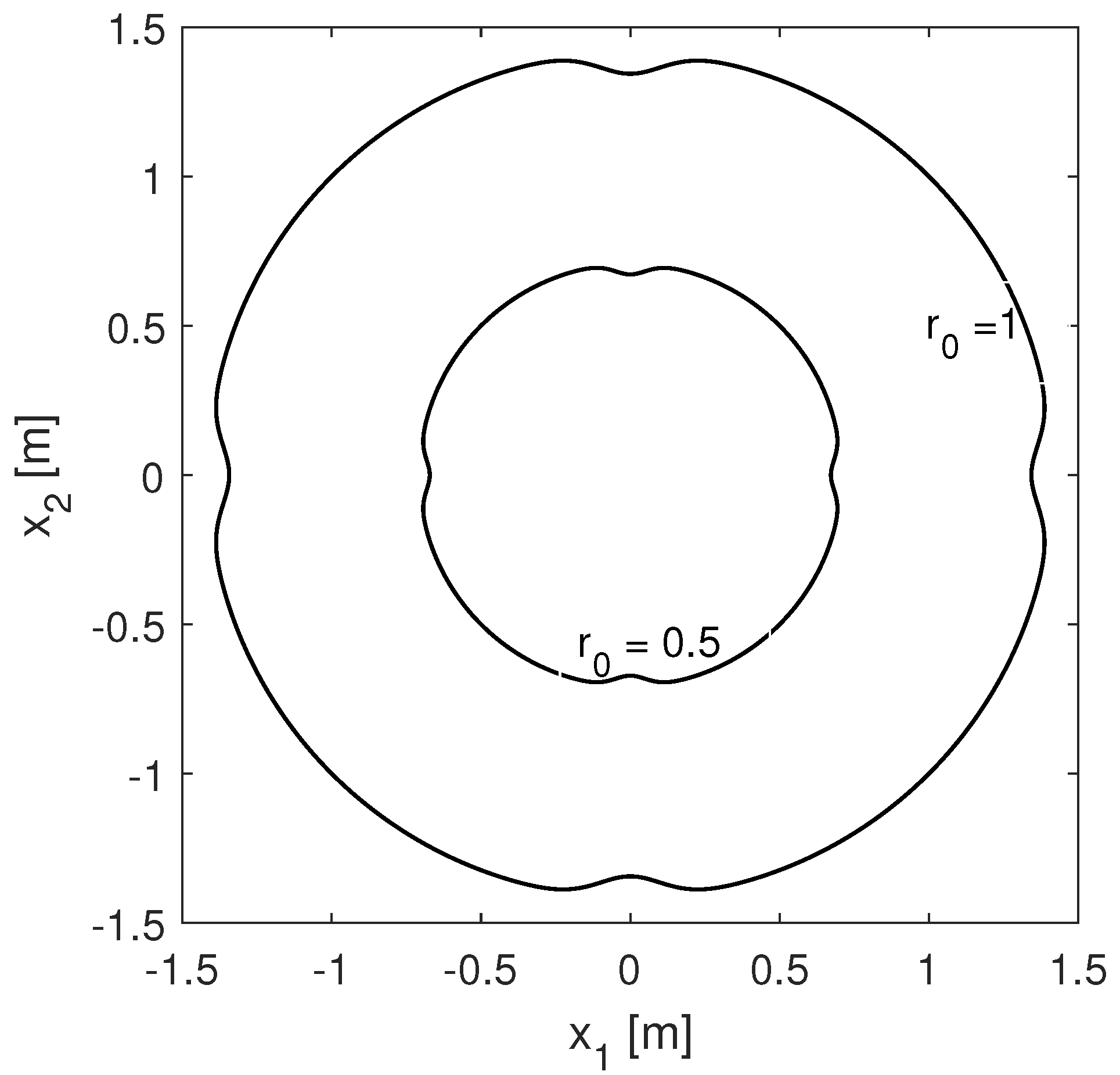
For the case at hand, inspired by the analysis described in [21], we identify a central zone ${\mathsf{\Omega }}^{*}$ of the domain $\mathsf{\Omega }$, in which the projected stress is a plane pressure. ${\mathsf{\Omega }}^{*}$ is delimited by a curve $\Gamma$ defined as

$$r_c\left(\theta \right)=r_0\sqrt{2}(1-\alpha {\left(cos\left(2\theta \right)\right)}^P)$$

(25)

where $r_0$ is a parameter, $\alpha$ is set to $0.05$ and P to 40. In Figure 5 we show the contour $r_c$ obtained for two representative values of $r_0$, namely $r_0=0.5$ and $r_0=1$.

Inside ${\mathsf{\Omega }}^{*}$, the Pucher stress is assumed as isotropic, that is

$$\mathbf{S}=-p_0({\mathbf{e}}_1\otimes {\mathbf{e}}_1+{\mathbf{e}}_2\otimes {\mathbf{e}}_2).$$

(26)

The corresponding stress potential is therefore easily computed as

$$F=-\frac{1}{2}{p}_0(x_1^2+x_2^2),$$

(27)

where $p_0$ is a parameter defining the intensity of the stress potential (i.e., of the stress) that will be subsequently optimized. In the external zone ${\mathsf{\Omega }}_{ext}$ the stress is assumed to be quasi-uniaxial in the radial direction. This means that, on defining $\widehat{\mathbf{r}}$ as the direction of the radii emanating from the geometrical center of the domain and directed toward the external boundary, the stress in ${\mathsf{\Omega }}_{ext}$ can be written as

$$\mathbf{S}=-\sigma \left(s\right)\widehat{\mathbf{r}}\otimes \widehat{\mathbf{r}}+\epsilon {\sigma }_0\widehat{\mathbf{t}}\otimes \widehat{\mathbf{t}}$$

(28)

where $\sigma \left(s\right)$ is related to $p_0$ and denotes the stress intensity along the radius, and $\epsilon {\sigma }_0$ is a small stress which has the function to give a small extra-curvature to the potential in the direction $\widehat{\mathbf{t}}$ orthogonal to $\widehat{\mathbf{r}}$, in order to preserve the ellipticity of Equation (6) when solved for the shape $f(x_1,x_2)$.

The stress potential associated to the stress distribution (28) in the external zone is obtained by imposing a linear growth in the radial direction, enforcing the continuity of the potential F and of its slope across the curve $\Gamma$:

$$F_{ext}=\nabla F_{int}{{|}_{\Gamma }·\widehat{\mathbf{r}}s+F|}_{\Gamma }-\epsilon \frac{{\sigma }_0}{2}{s}^2,$$

(29)

where s is a parameter indicating the distance from $\Gamma$ along the radius.

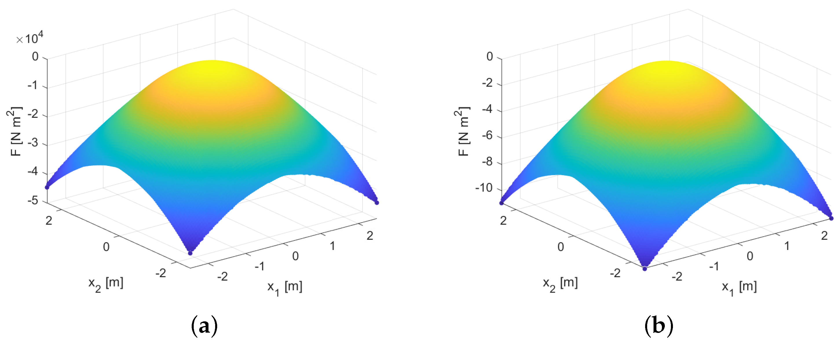
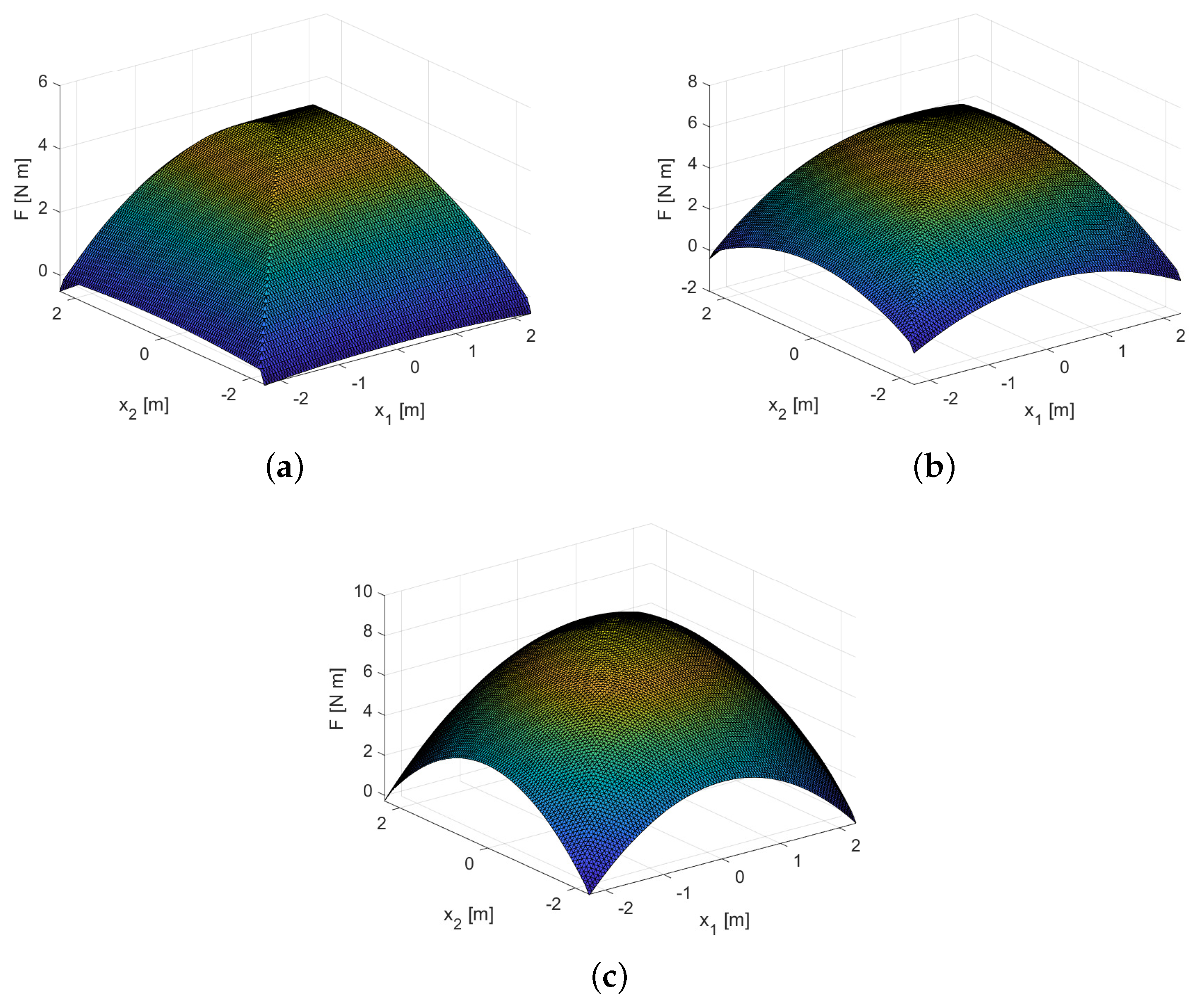
In Figure 6, we show the the stress potential for two representative values of $r_0$. Adopting these two shapes as the stress potential, and taking as boundary condition for the membrane geometry $f(x_1,x_2)$ the value of the rise of the middle surface between the intrados and the extrados of the vault, Equation (6) can be solved using LSM, as described in Section 3.2. 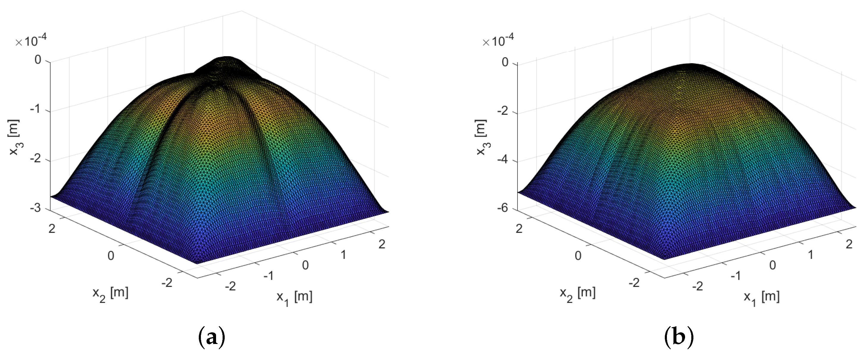By constructing a structured triangulation based on a regular node distribution over the planform $\mathsf{\Omega }$, the membrane shapes corresponding to the stress potentials of Figure 6, are represented in Figure 7.

Figure 7 gives an idea on how the choice of the parameter $r_0$ (and thus, the extension of the central zone characterized by a biaxial stress state) influences the final shape of the membrane geometry. In the second case ($r_0=1$), the membrane geometry resembles the shape of a cloister vault more than in the case of $r_0=0.5$. It is also evident that the height of the two shapes (in the direction of the $x_3$-axis) are not comparable with the height of the cloister vault defined from Equations (23) and (24), which is $2.13$ m.

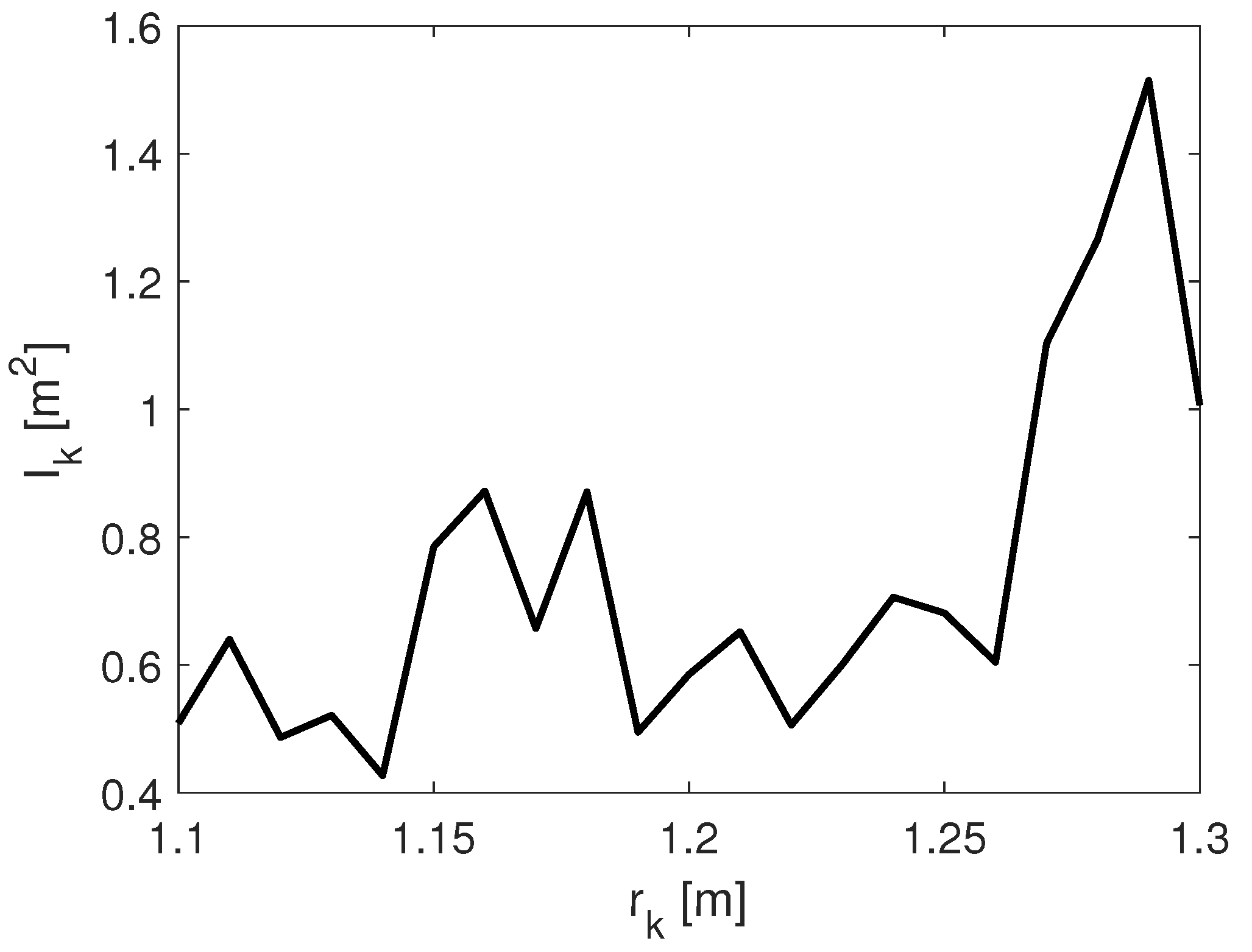
The minimization of the error function (20) with respect to the parameters $p_0$ and $r_0$ is performed as follows: first, $r_0$ is given a finite number of values in the range $[0,L]$, i.e., $r_{0,k}=1.1+k0.01,k=0,\dots ,20$. Then, for each value of $r_{0,k}$, we search the $p_{0,k}$ that minimizes $I_k=I_k(r_{0,k},p_{0,k})$. In Figure 8 we show the considered values of the $r_{0,k}$ on the horizontal axis, and on the vertical axes we show the corresponding optimal value of $I_k$.

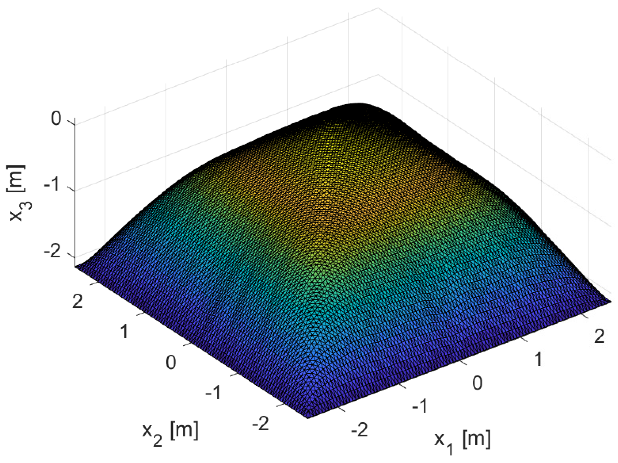
The lowest value of $I_k$ is reached when $r_k=1.14$, which correspond to $p_{0,k}=3.45\times {10}^3$. Therefore the parameters of the stress potential are fixed to $r_0=1.14$ and $p_0=3.45\times {10}^3$. The best-fitting membrane geometry is then represented in Figure 9.

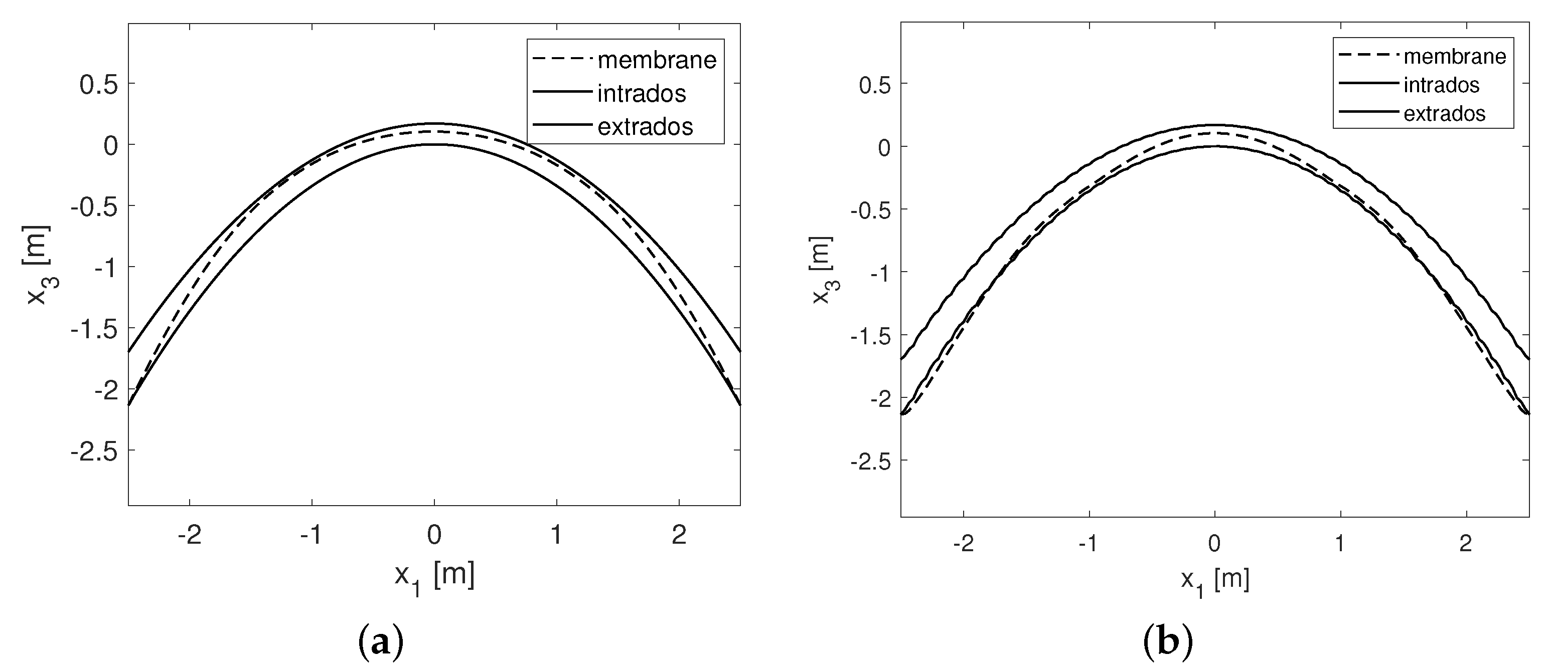
In Figure 10 we also show two sections of the membrane and of the intrados and extrados, the first one taken at $x_2=0$, and the second one taken along the diagonal of the domain, that is for $x_2=-x_1$.

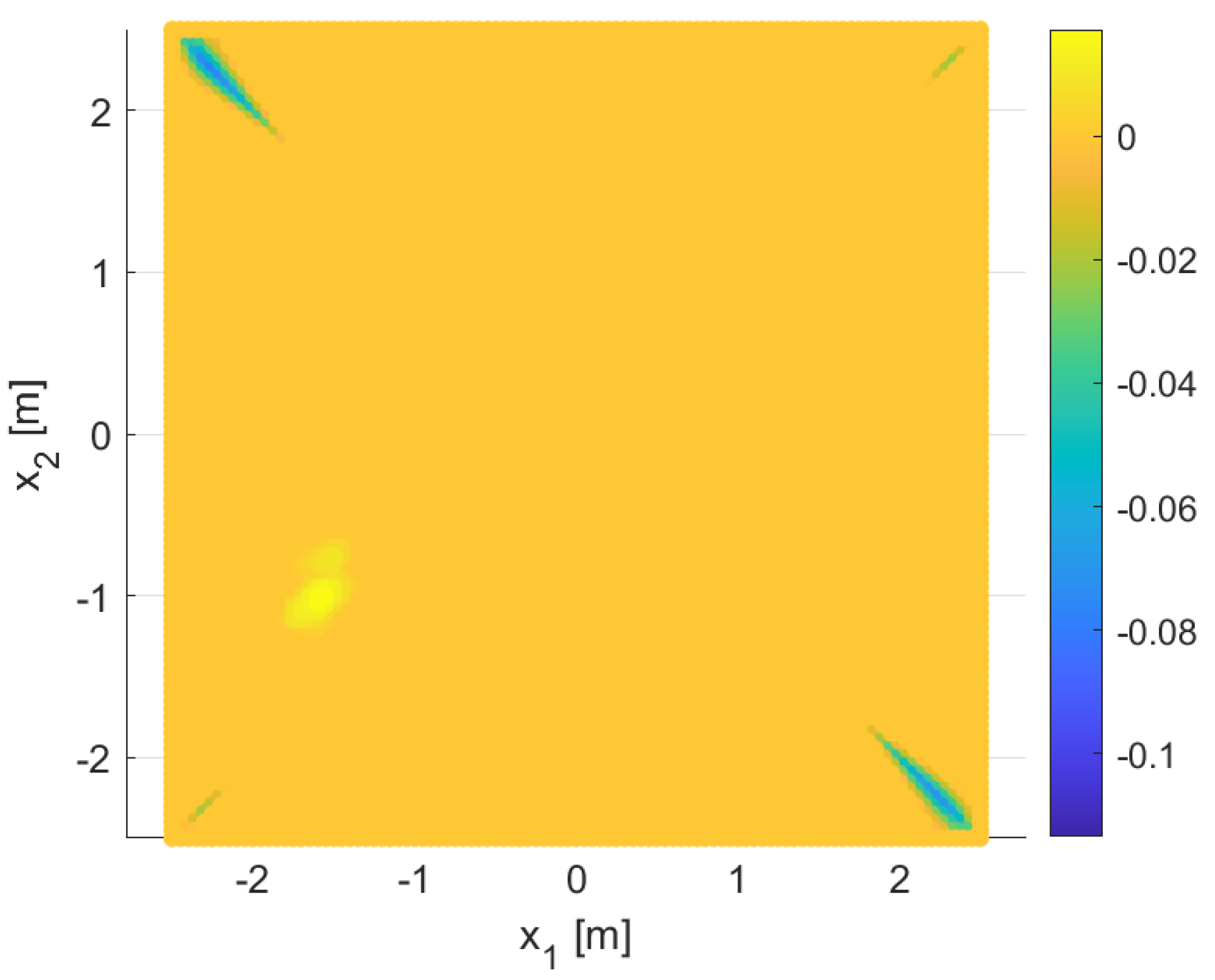
We notice from Figure 10b that some points of the membrane fall outside the volume of the vault; this is confirmed also by Figure 11, where we show the color map of the function $g(x_1,x_2)$ defined as

$$g(x_1,x_2)=\left\{\begin{array}{c}\begin{array}{cc}f-f_{intr}\hfill & \hfill f<f_{intr}\\ 0\hfill & \hfill f_{intr}<f<f_{extr}\\ f-f_{extr}\hfill & \hfill f>f_{extr}\end{array}\hfill \end{array}\right.$$

(30)

for which positive values indicate points in which the membrane shape is above the extrados of the vault, negative values indicate when the membrane is below the intrados, and vanishing values indicate nodes that are comprised within the volume of the vault.

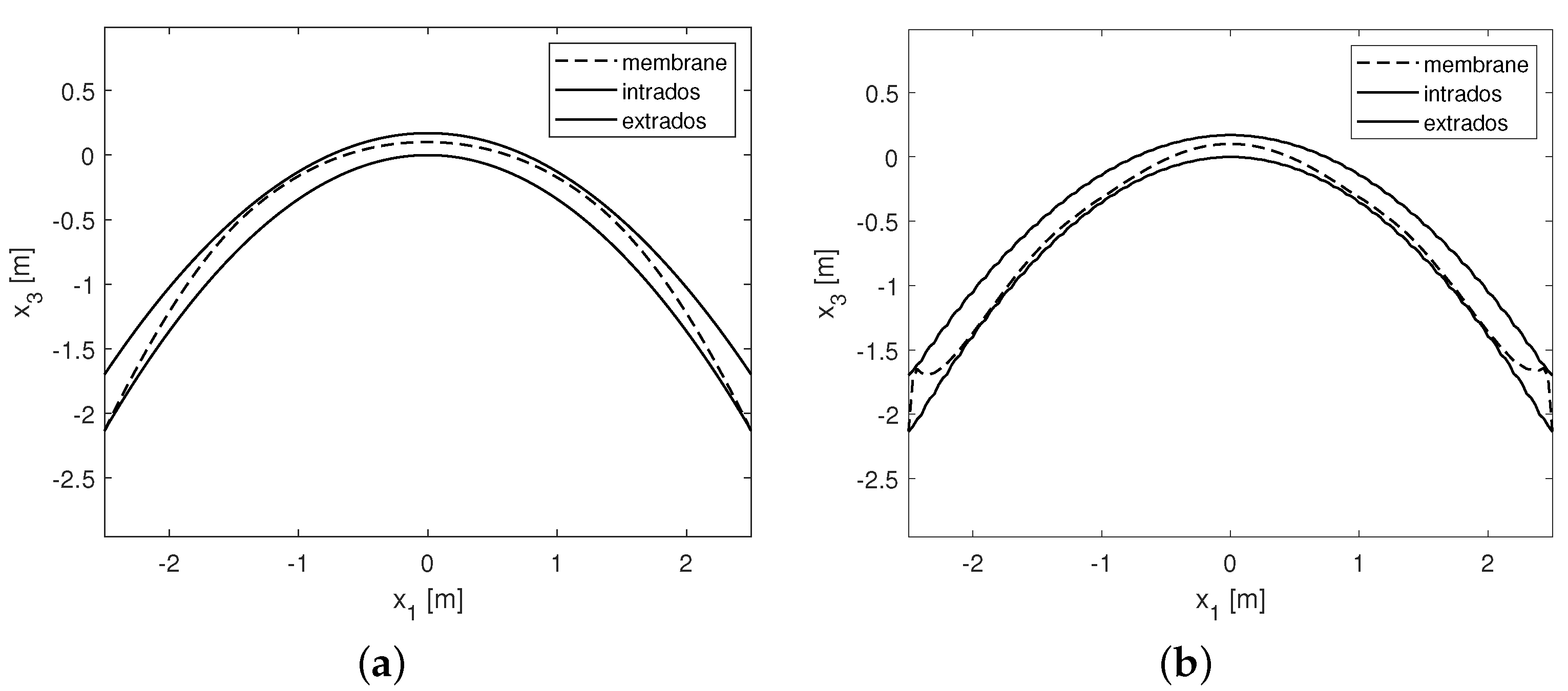
We then perform the last step of the optimization, with respect to the boundary values of the membrane shape, obtaining a new membrane geometry whose sections for $x_2=0$ and $x_2=-x_1$ are shown in Figure 12. In this case, we notice that the points that were falling outside the volume of the vault before this optimization step, are now comprised between the intrados and the extrados.

The whole algorithm has been repeated assuming the same loads, but reduced thickness, in order to assess the geometrical safety factor. The higher thickness reduction for which the proposed algorithm still produces admissible solutions, in the sense of Limit Analysis, is $38\%$ of the original thickness, corresponding to a geometrical safety factor of $1.61$.

4.2. Cross Vault of the Anterior Portico of the Church of St. Pietro in Vineis in Anagni

In this section we consider the case of the anterior portico of the church of San Pietro in Vineis in Anagni. The portico consists of three similar cross vaults: the geometrical description of each vault, referring for notation to Figure 13 and Figure 14, is given by:

$$f_{intr}(x_1,x_2)=\left\{\begin{array}{c}\begin{array}{cc}4\frac{h_{i,1}}{b_i^2}\left(\frac{b_i^2}{4}-x_2^2\right)+4\frac{h_i-h_{i,1}}{a_i^2}\left(\frac{a_i^2}{4}-x_1^2\right)\hfill & \hfill (x_1,x_2)\in ({\mathsf{\Omega }}_1\cup {\mathsf{\Omega }}_3)\\ 4\frac{h_{i,2}}{b_i^2}\left(\frac{b_i^2}{4}-x_2^2\right)+4\frac{h_i-h_{i,2}}{a_i^2}\left(\frac{a_i^2}{4}-x_1^2\right)\hfill & \hfill (x_1,x_2)\in ({\mathsf{\Omega }}_2\cup {\mathsf{\Omega }}_4)\end{array}\hfill \end{array}\right.$$

(31)

$$f_{extr}(x_1,x_2)=\left\{\begin{array}{c}\begin{array}{cc}4\frac{h_{e,1}}{b_e^2}\left(\frac{b_e^2}{4}-x_2^2\right)+4\frac{h_e-h_{e,1}}{a_e^2}\left(\frac{a_e^2}{4}-x_1^2\right)\hfill & \hfill (x_1,x_2)\in ({\mathsf{\Omega }}_1\cup {\mathsf{\Omega }}_3)\\ 4\frac{h_{e,2}}{b_e^2}\left(\frac{b_e^2}{4}-x_2^2\right)+4\frac{h_e-h_{e,2}}{a_e^2}\left(\frac{a_e^2}{4}-x_1^2\right)\hfill & \hfill (x_1,x_2)\in ({\mathsf{\Omega }}_2\cup {\mathsf{\Omega }}_4)\end{array}\hfill \end{array}\right.$$

(32)

The values given to the geometrical parameters introduced in Equations (31) and (32), are reported in

Table 1. Intrados and extrados data referring to notation in Figure 14.

$a_i$ [m]	$b_i$ [m]	$h_i$ [m]	$h_{i,1}$ [m]	$h_{i,2}$ [m]
4.68	4.59	2.16	1.84	2.05
$a_e$ [m]	$b_e$ [m]	$h_e$ [m]	$h_{e,1}$ [m]	$h_{e,2}$ [m]
4.88	4.79	2.36	2.04	2.25

.

For this kind of vault a concave membrane surface comprised between the intrados and the extrados does not exist; as a consequence, using Equation (6) with a known shape and unknown stress potential would lead to a non-elliptic problem, that cannot be solved using a FEM-like procedure. The inverse problem, consisting in the search of the shape corresponding to a given concave stress potential, is elliptic instead, and the FEM-like procedure proposed in [21] can be applied.

It is a well-known result (see [27]) that the stress potential corresponding to a standard cross vault has the shape of a cloister vault. The case at hand, however, is not a standard cross vault since there is a curvature not only orthogonally to each median of the planform, but also in the median direction. We expect, therefore, a biaxial stress field, with components both along the direction of the medians, and in its orthogonal direction.

We propose therefore the following stress potential $F(x_1,x_2)$

$$F(x_1,x_2)=\left\{\begin{array}{c}\begin{array}{cc}-{\alpha }_0\left[\left(x_1^2-\frac{a_i^2}{4}\right)+\beta \left(x_2^2-\frac{b_i^2}{4}\right)\right]\hfill & \hfill (x_1,x_2)\in ({\mathsf{\Omega }}_1\cup {\mathsf{\Omega }}_3)\\ -{\alpha }_0\left[\left(x_2^2-\frac{b_i^2}{4}\right)+\beta \left(x_1^2-\frac{a_i^2}{4}\right)\right]\hfill & \hfill (x_1,x_2)\in ({\mathsf{\Omega }}_2\cup {\mathsf{\Omega }}_4)\end{array}\hfill \end{array}\right.$$

(33)

For sake of example, in Figure 15 we present three different stress potentials obtained for $\beta =0$, $\beta =0.3$, and $\beta =0.7$ and ${\alpha }_0=1$.

We assume the same definition of the error introduced in Equation (20) and evaluate it for different values of $\beta$, and then minimizing $I_k$ with respect to ${\alpha }_0$. The values of $\beta$ considered in this case are

$${\beta }_k=0.3+k0.02,k=0,...,10$$

(34)

The corresponding plot of the error $I_k$ versus $\beta$ is reported in Figure 16 in a logarithmic scale along the error axis.

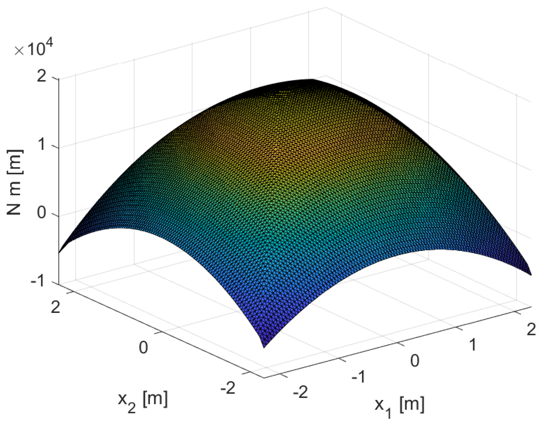
The minimum occurs at $\beta =0.4$, and corresponds to an error of $3.94\times {10}^{-2}$. The corresponding stress potential is shown in Figure 17.

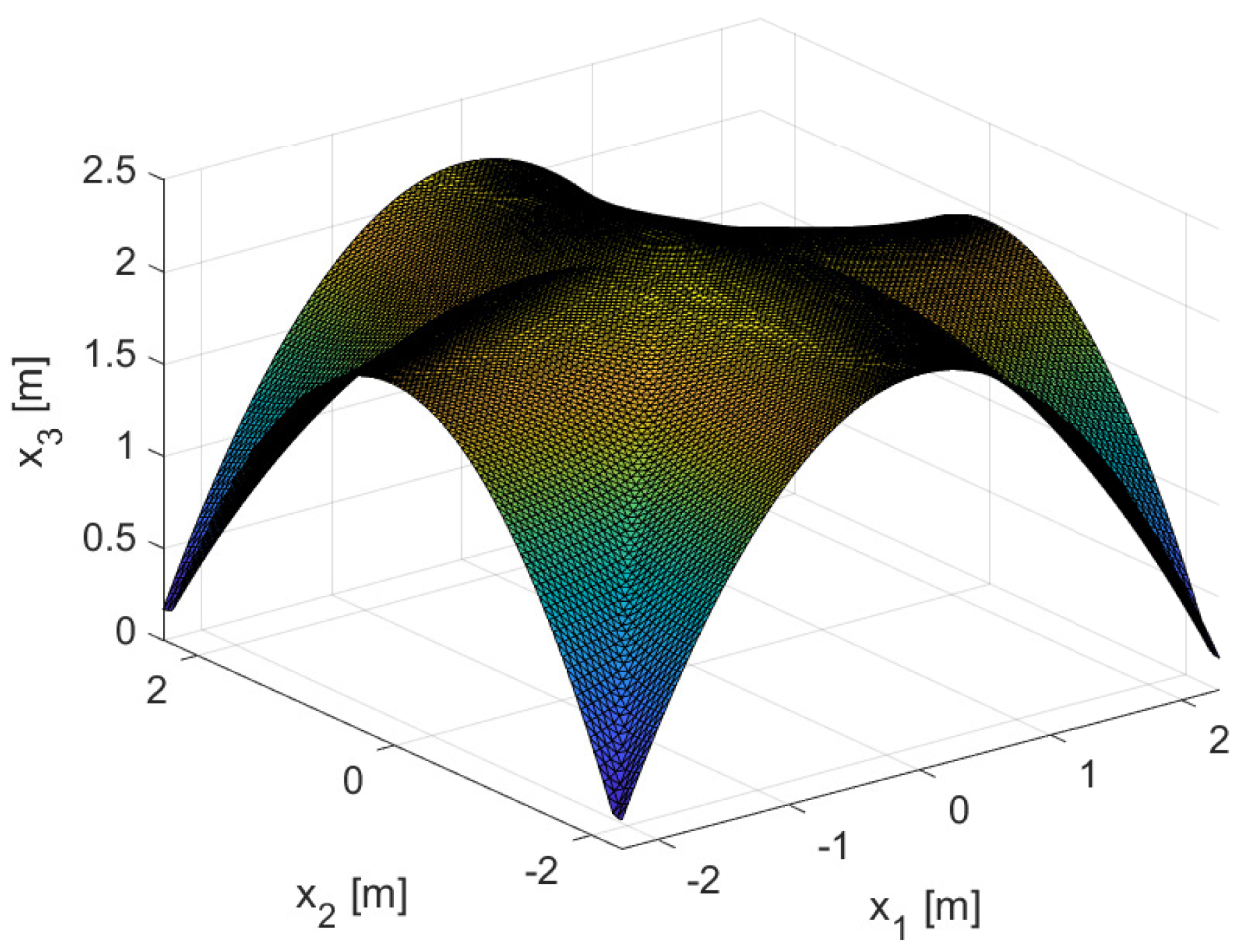
The corresponding shape of the membrane, obtained through the numerical solution of Equation (6), and imposing as boundary values for $f(x_1,x_2)$ the values of the midsurface (between the intrados and the extrados), is shown in Figure 18.

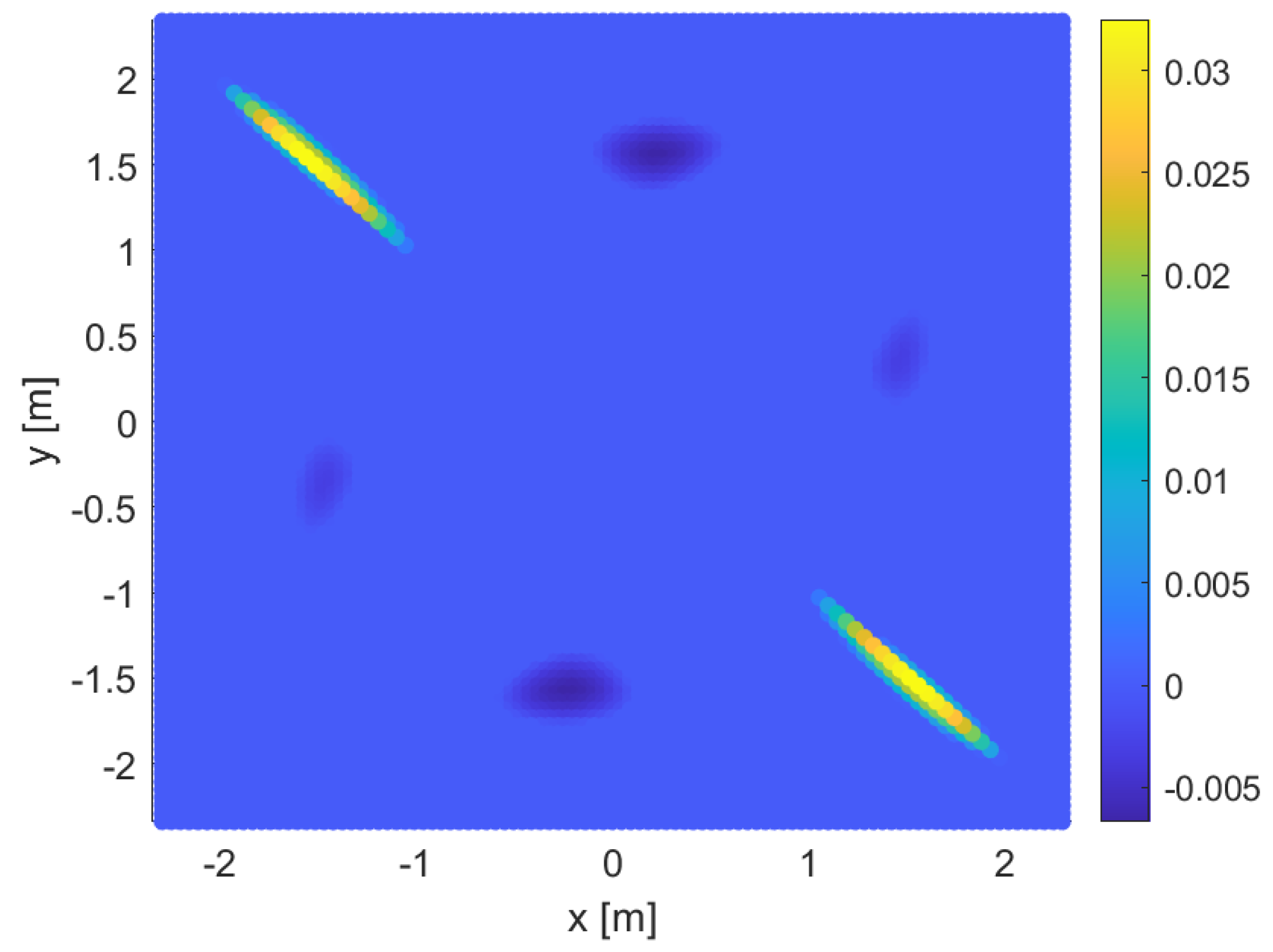
To evaluate the position of the membrane surface after this first optimization phase, we show in Figure 19 the colormap of $g(x_1,x_2)$, defined like in Equation (30), applied to this case study. The presence in Figure 19 of points for which the error function is non zero indicates that the membrane found after the first optimization step is not fully comprised between the intrados and the extrados. Therefore we need a further optimization step to achieve this goal.

The second step of the minimization process is then performed with respect to the boundary values of the membrane shape. The value of the error function $I=I\left({\overline{\mathbf{f}}}_B\right)$, obtained as a result of the second optimization phase, is zero everywhere, meaning that the membrane fits in-between the bounding surfaces of the vault.

For sake of example, we show in Figure 20 a graph of a section of the intrados, the extrados and the membrane shape along the diagonal line $x_2=-\frac{b_i}{a_i}{x}_1$, that, after the first minimization phase, exhibits points lying outside the vault geometry. As expected, there are no points of the membrane section falling outside the geometry of the vault.

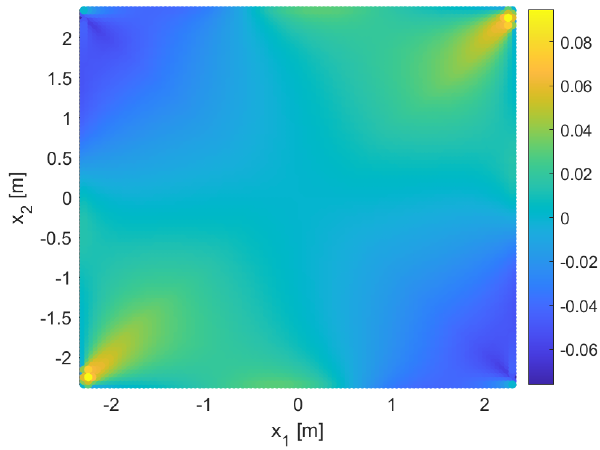
The influence of changing the boundary values ${\overline{\mathbf{f}}}_B$ is made evident by the color map of the difference $h(x_1,x_2)$ defined as

$$h(x_1,x_2)=f_{opt}(x_1,x_2)-f(x_1,x_2)$$

(35)

and shown in Figure 21, where f is the membrane geometry at the end of the first minimization step, and $f_{opt}$ is the geometry after the final minimization with respect to the boundary conditions.

From Figure 21 we see that the main effects of the modification of the boundary conditions is that the rise change of the membrane, represented by Equation (35), after the second optimization phase, are visible mainly in the boundary part of the domain, as expected from the discussion about elliptic partial differential equations. Moreover, we see that $h(x_1,x_2)$ is negative in the lowest-right and upper-left corners, meaning that the membrane rise is diminished after this optimization, fixing the error shown in Figure 19.

In order to quantify the Geometrical Safety Factor for this vault, the algorithm has been repeated progressively reducing the thickness. The maximum possible reduction, given the assumed shape for the stress potential, is $36\%$, corresponding to a GSF $=1.56$.

4.3. Discussion

Concerning the algorithm adopted in both examples, we point out that it is an automatic procedure that is easily adaptable to the specific case. The only different step between the proposed algorithms, beyond the geometries of the vault, is the parametric description of the stress potential, which is specific to each case study, and consists, from an operative point of view, in replacing a computer routine to another one.

Concerning the Geometrical Safety Factor, computed at the end of each application, we remark thaat it is an intrinsic characteristic of each structure, and does not depend, in general, on the adopted membrane shape or its associated equilibrated stress. With computational models, such as MEA, it is only possible to try to find the best value, that, in turn, is associated to specific choices on the stress potential (i.e., its shape, or its parametric description), or on the discretization, or on the specific algorithm.

In our examples, we made two precise choices for the shape of the stress potential, based on experience and on literature examples. A richer description of the stress potential could have improved the obtained value of the Geometrical Safety Factor, at the price of a more complicate and slow optimization algorithm, especially for the first optimization pahse, which is characterized, for each evaluation of the objective function, by a matrix inversion, whose computational cost, in turn, depends in the adopted discretization. Therefore, the proposed values for the GSF have to be considered as conservative values, and could be improved by using more refined optimization algorithms, not yet developed in the framework of the Membrane Equilibrium Analysis.

5. Conclusions

In this work we present a method for the assessment of the equilibrium of masonry vaults based on the search for a suitable membrane shape in equilibrium with a given compressive stress field. The membrane shape is required to be entirely comprised between the intrados and the extrados of a vault, according to the Safe Theorem of Limit Analysis.

The proposed method aims at finding a concave stress potential in equilibrium with the applied loads on a membrane geometry entirely included in the volume of the membrane. To match this objective, the algorithm starts from a parametric description of the stress potential and follows two subsequent optimization steps: in the first one, the parameters of the stress potential are optimized, through the solution of the transverse equilibrium equation of a membrane, assuming fixed boundary conditions for the membrane shape; in the second step, the boundary values of the membrane shape are selected, by minimizing an error function defined as a quadratic approximation of the characteristic function over the planform of the membrane.

The main advantage of this approach is the possibility of solving, in each optimization phase, an elliptic problem, since the stress potential is assumed to be known and concave. This strategy permits the solution of problems for which a concave shape, comprised in the volume of the vault, does not exist, such as in the case of cross vaults. For such vaults, in fact, the search of a stress field starting from a possible membrane shape (in-between the intrados and the extrados of the vault) is described by a non-elliptic second order partial differential equation, that cannot be solved by the simple inversion of the matrix arising from its discretization.

The algorithm is applied to two benchmarks: a cloister vault, with the dimensions of a vault in Palazzo Caracciolo di Avellino, in Naples, and the cross vault of the anterior portico of San Pietro in Vineis, in Anagni (Italy). For both problems, given a suitable parametric description for the stress potential, a membrane shape is found, fulfilling the requirements of Limit Analysis with acceptable geometrical safety factors, demonstrating the validity of the proposed methodology in assessing the stability of vaults.

Future perspectives for this work will include the development of an algorithm for which the stress potential and the membrane shape are optimized simultaneously, under the constraints of the equilibrium and of the Safe Theorem of Limit Analysis.