Flow Duration Curves from Surface Reflectance in the Near Infrared Band


Abstract
1. Introduction
2. Materials and Methods
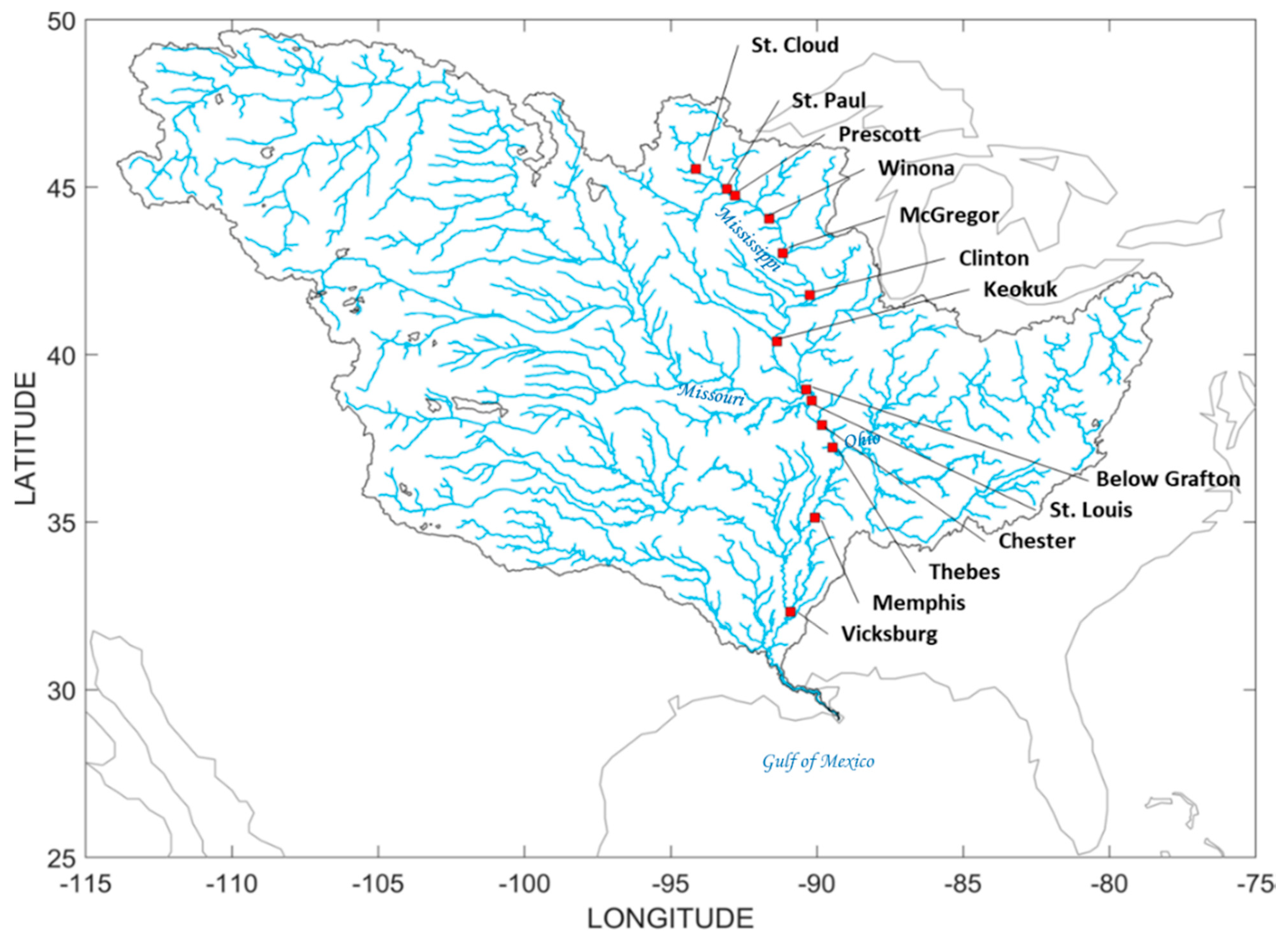
2.1. Study Area and Datasets
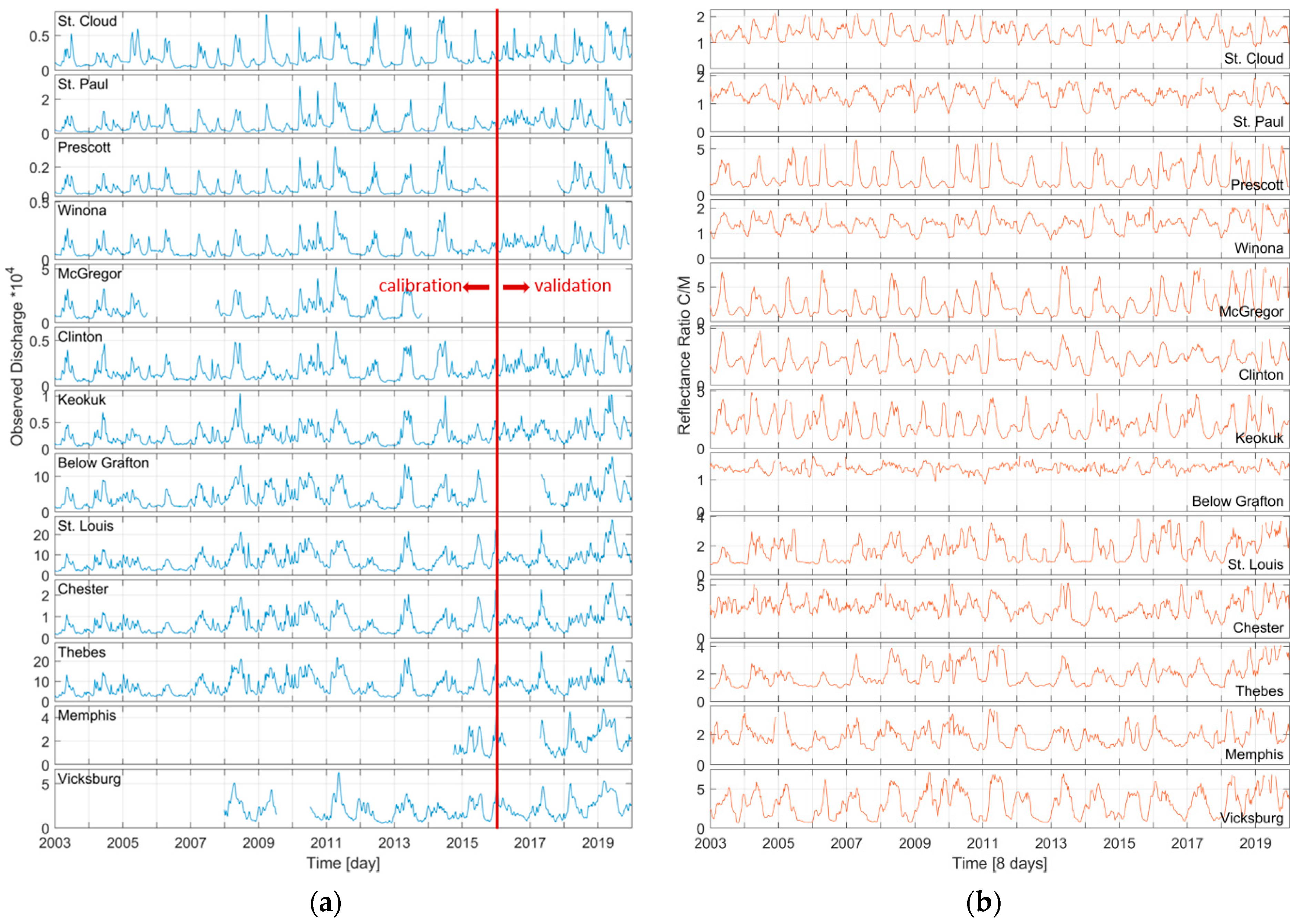
2.1.1. In Situ Dataset
2.1.2. Satellite Dataset
2.2. Methods
2.2.1. Estimation of the Reflectance Ratio
- Cut the MODIS images over a square of size proportional to the width of the river (the side ranges from 0.05 to 0.11 km) and centered on the selected site.
- Calculate the temporal coefficient of variation for every pixel of the box considering the set of available MODIS images.
- Calculate, for each image, the spatial average of the reflectance considering the pixels with the coefficient of variation lower than the 5th percentile; this represents the time series of dry pixel (C) at a given location.
- Select a buffer of 1 km around the river and calculate all possible C/M ratios by considering M values of the pixels within the buffer and the average C obtained at step (3).
- Compare every C/M time series against the discharge recorder by the ground monitoring network and calculate the coefficient of correlation.
- Identify the C/M combination and, hence, M pixel that maximizes the coefficient of correlation.
2.2.2. FDC Estimation
2.2.3. Data Consistency
2.3. Evaluation of the Results
- Root mean square error, RMSE, the second sample moment of the residuals (or differences) between predicted and observed values. It ranges from 0 (perfect fit) to +∞ (low performances).
- Relative RMSE, rRMSE, defined as:
- Normalized RMSE, NRMSE, defined as:
- The Nash–Sutcliffe efficiency [27], NSE, defined as:
3. Results
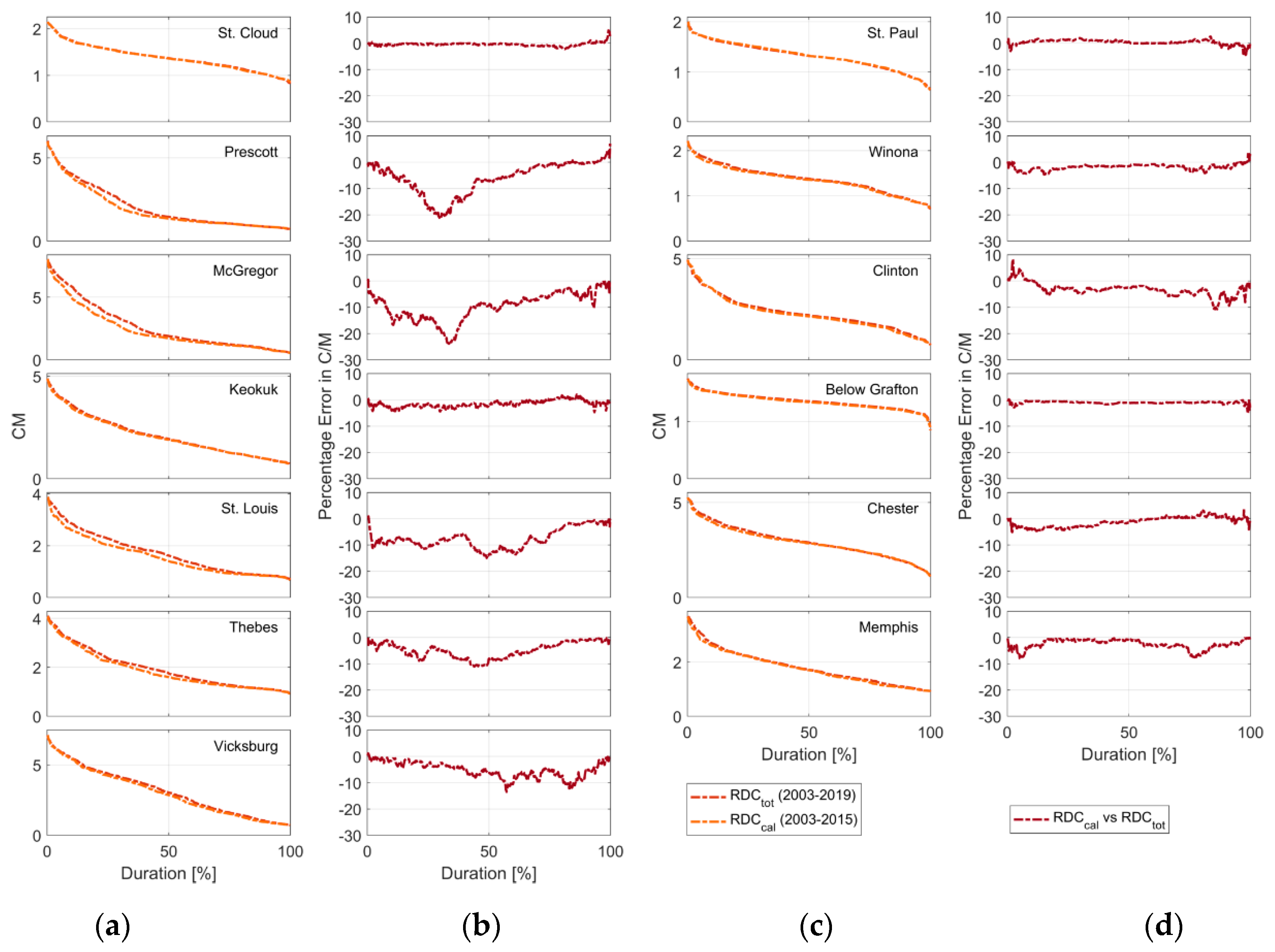
3.1. FDCs and RDCs Definition Based on Available Datasets
3.2. Comparison in Terms of River Discharge: Calibration Phase
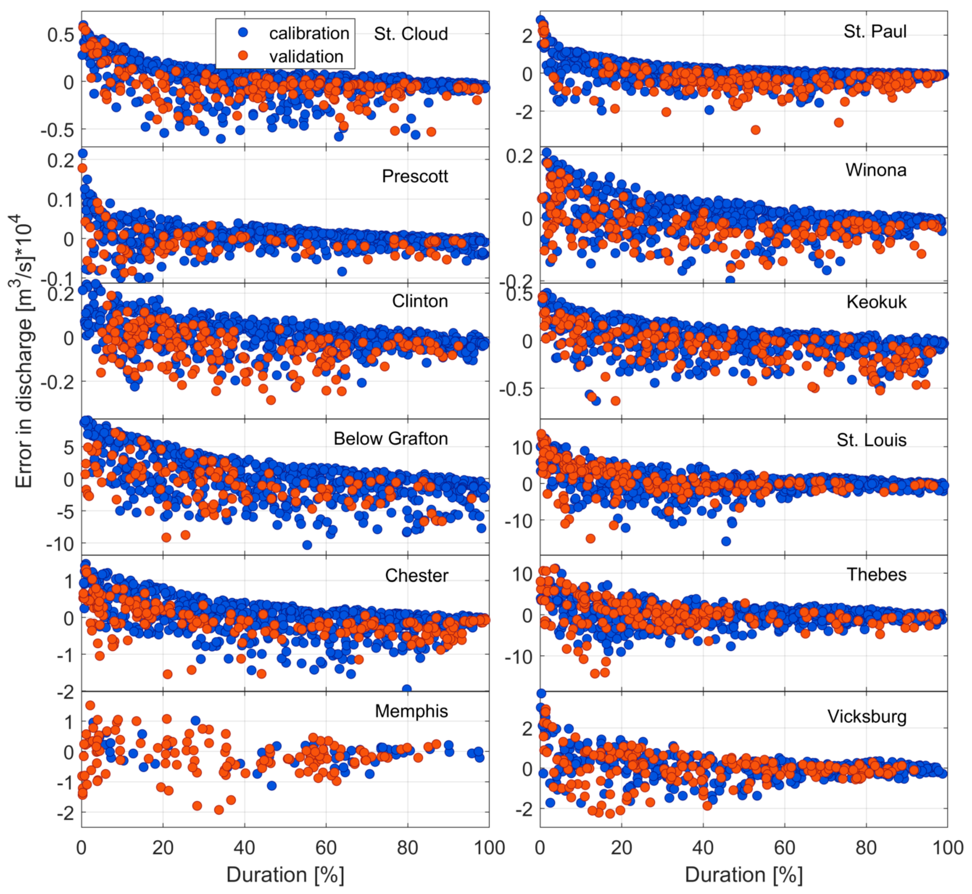
3.3. Comparison in Terms of River Discharge: Validation Phase
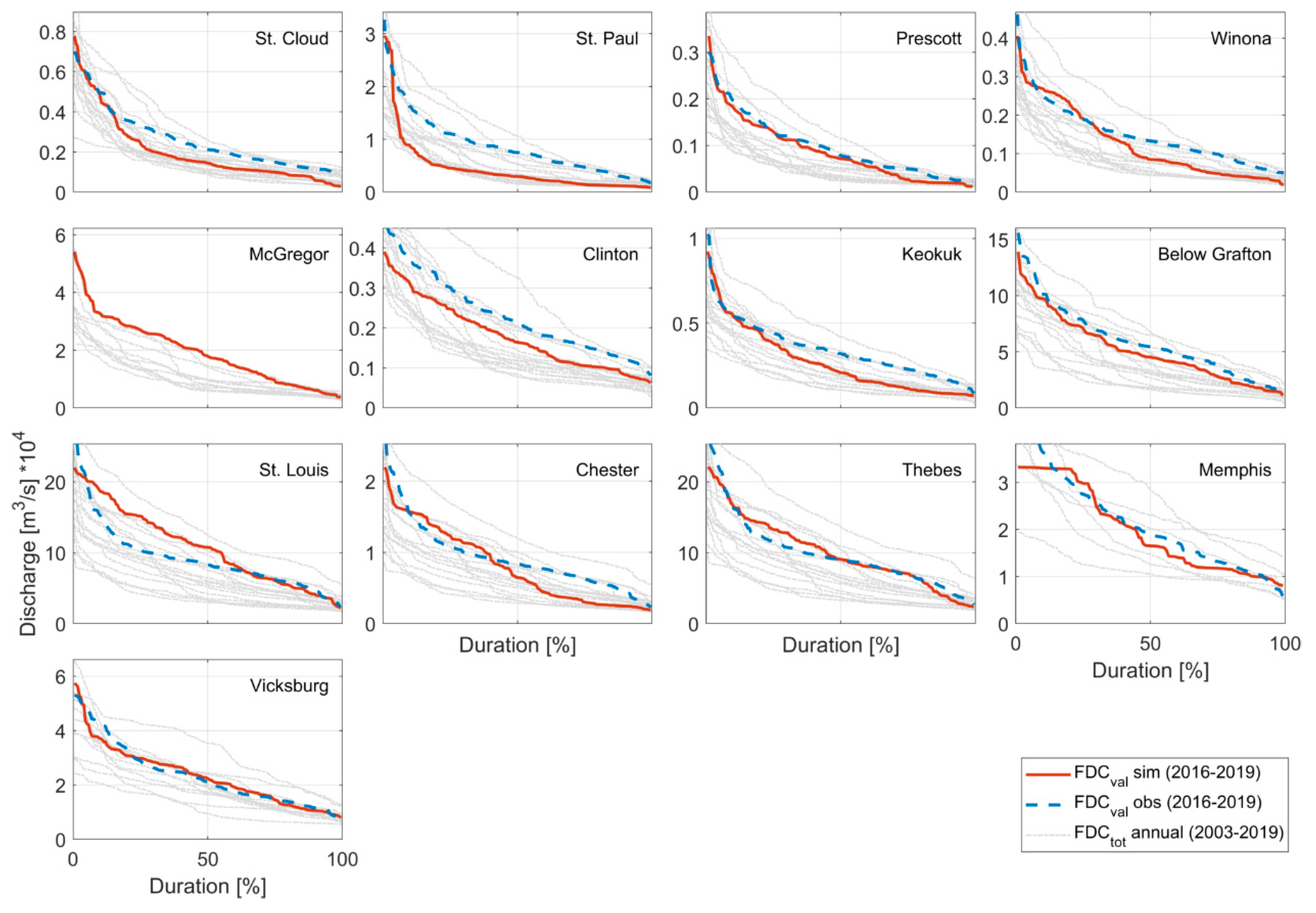
3.4. FDCs in the Validation Phase: Evaluation of the Performances
4. Discussion
5. Conclusions
Supplementary Materials
Author Contributions
Funding
Institutional Review Board Statement
Informed Consent Statement
Data Availability Statement
Acknowledgments
Conflicts of Interest
References
- Vogel, R.M.; Fennessey, N.M. Flow duration curves II: A review of applications in water resources planning 1. JAWRA J. Am. Water Resour. Assoc. 1995, 31, 1029–1039. [Google Scholar] [CrossRef] [Scilit]
- Pugliese, A.; Castellarin, A.; Brath, A. Geostatistical prediction of flow–duration curves in an index-flow framework. Hydrol. Earth Syst. Sci. 2014, 18, 3801–3816. [Google Scholar] [CrossRef] [Scilit]
- Castellarin, A.; Persiano, S.; Pugliese, A.; Aloe, A.; Skøien, J.O.; Pistocchi, A. Prediction of streamflow regimes over large geographical areas: Interpolated flow–duration curves for the Danube region. Hydrol. Sci. J. 2018, 63, 845–861. [Google Scholar] [CrossRef] [Scilit]
- Booker, D.J.; Snelder, T.H. Comparing methods for estimating flow duration curves at ungauged sites. J. Hydrol. 2012, 434–435, 78–94. [Google Scholar] [CrossRef] [Scilit]
- Domeneghetti, A.; Tarpanelli, A.; Grimaldi, L.; Brath, A.; Schumann, G. Flow Duration Curve from Satellite: Potential of a Lifetime SWOT Mission. Remote Sens. 2018, 10, 1107. [Google Scholar] [CrossRef] [Scilit]
- Domeneghetti, A.; Schumann, G.; Tarpanelli, A. Preface: Remote Sensing for Flood Mapping and Monitoring of Flood Dynamics. Remote Sens. 2019, 11, 943. [Google Scholar] [CrossRef] [Scilit]
- Tourian, M.J.; Sneeuw, N.; Bárdossy, A. A quantile function approach to discharge estimation from satellite altimetry (ENVISAT). Water Resour. Res. 2013, 49, 4174–4186. [Google Scholar] [CrossRef] [Scilit]
- Brakenridge, G.R.; Nghiem, S.V.; Anderson, E.; Chien, S. Space-based measurement of river runoff. Eos Trans. AGU 2005, 86, 185–188. [Google Scholar] [CrossRef] [Scilit]
- Tarpanelli, A.; Brocca, L.; Lacava, T.; Melone, F.; Moramarco, T.; Faruolo, M.; Pergola, N.; Tramutoli, V. Toward the estimation of river discharge variations using MODIS data in ungauged basins. Remote Sens. Environ. 2013, 136, 47–55. [Google Scholar] [CrossRef] [Scilit]
- Van Dijk, A.I.J.M.; Brakenridge, G.R.; Kettner, A.J.; Beck, H.E.; De Groeve, T.; Schellekens, J. River gauging at global scale using optical and passive microwave remote sensing. Water Resour. Res. 2016, 52, 6404–6418. [Google Scholar] [CrossRef] [Scilit]
- Li, H.; Li, H.; Wang, J.; Hao, X. Extending the Ability of Near-Infrared Images to Monitor Small River Discharge on the Northeastern Tibetan Plateau. Water Resour. Res. 2019, 55, 8404–8421. [Google Scholar] [CrossRef] [Scilit]
- Shi, Z.; Chen, Y.; Liu, Q.; Huang, C. Discharge Estimation Using Harmonized Landsat and Sentinel-2 Product: Case Studies in the Murray Darling Basin. Remote Sens. 2020, 12, 2810. [Google Scholar] [CrossRef] [Scilit]
- Sahoo, D.P.; Sahoo, B.; Tiwari, M.K. Copula-based probabilistic spectral algorithms for high-frequent streamflow estimation. Remote Sens. Environ. 2020, 251, 112092. [Google Scholar] [CrossRef] [Scilit]
- Tarpanelli, A.; Amarnath, G.; Brocca, L.; Massari, C.; Moramarco, T. Discharge estimation and forecasting by MODIS and altimetry data in Niger-Benue River. Remote Sens. Environ. 2017, 195, 96–106. [Google Scholar] [CrossRef] [Scilit]
- Ghizzoni, T.; Roth, G.; Rudari, R. Multisite flooding hazard assessment in the Upper Mississippi River. J. Hydrol. 2012, 412–413, 101–113. [Google Scholar] [CrossRef] [Scilit]
- United States Geological Survey, USGS. Available online: https://waterdata.usgs.gov/nwis/sw (accessed on 10 January 2021).
- United States Geological Survey, USGS. Available online: https://search.earthdata.nasa.gov/ (accessed on 22 September 2020).
- Vermote, E.F.; Kotchenova, S.Y. MOD09 (Surface Reflectance) User’s Guide, Version 1.1. March 2008. Available online: https://patarnott.com/satsens/pdf/MOD09_UserGuide_v1_2.pdf (accessed on 12 April 2021).
- Huang, C.; Chen, Y.; Zhang, S.; Wu, J. Detecting, extracting, and monitoring surface water from space using optical sensors: A review. Rev. Geophys. 2018, 56, 333–360. [Google Scholar] [CrossRef] [Scilit]
- McFeeters, S.K. The use of the Normalized Difference Water Index (NDWI) in the delineation of open water features. Int. J. Remote Sens. 1996, 17, 1425–1432. [Google Scholar] [CrossRef] [Scilit]
- Yang, X.; Zhao, S.; Qin, X.; Zhao, N.; Liang, L. Mapping of urban surface water bodies from Sentinel-2 MSI imagery at 10 m resolution via NDWI-based image sharpening. Remote Sens. 2017, 9, 596. [Google Scholar] [CrossRef] [Scilit]
- Munasinghe, D.; Cohen, S.; Huang, Y.F.; Tsang, Y.P.; Zhang, J.; Fang, Z. Intercomparison of Satellite Remote Sensing-Based Flood Inundation Mapping Techniques. JAWRA J. Am. Water Resour. Assoc. 2018, 54, 834–846. [Google Scholar] [CrossRef] [Scilit]
- Nandi, I.; Srivastava, P.K.; Shah, K. Floodplain mapping through support vector machine and optical/infrared images from Landsat 8 OLI/TIRS sensors: Case study from Varanasi. Water Resour. Manag. 2017, 31, 1157–1171. [Google Scholar] [CrossRef] [Scilit]
- Tarpanelli, A.; Santi, E.; Tourian, M.J.; Filippucci, P.; Amarnath, G.; Brocca, L. Daily river discharge estimates by merging satellite optical sensors and radar altimetry through artificial neural network. IEEE Trans. Geosci. Remote 2018, 57, 329–341. [Google Scholar] [CrossRef] [Scilit]
- Tarpanelli, A.; Iodice, F.; Brocca, L.; Restano, M.; Benveniste, J. River flow monitoring by Sentinel-3 OLCI and MODIS: Comparison and combination. Remote Sens. 2020, 12, 3867. [Google Scholar] [CrossRef] [Scilit]
- Massey, F.J. The Kolmogorov-Smirnov Test for Goodness of Fit. J. Am. Stat. Assoc. 1951, 46, 68–78. [Google Scholar] [CrossRef]
- Nash, J.E.; Sutcliffe, J.V. River flow forecasting through conceptual models, part I: A discussion of principles. J. Hydrol. 1970, 10, 282–290. [Google Scholar] [CrossRef] [Scilit]
- Paris, A.; Dias de Paiva, R.; Santos da Silva, J.; Medeiros Moreira, D.; Calmant, S.; Garambois, P.-A.; Collischonn, W.; Bonnet, M.-P.; Seyler, F. Stage-discharge rating curves based on satellite altimetry and modeled discharge in the Amazon basin. Water Resour. Res. 2016, 52, 3787–3814. [Google Scholar] [CrossRef] [Scilit]
- Zakharova, E.A.; Krylenko, I.N.; Kouraev, A.V. Use of non-polar orbiting satellite radar altimeters of the Jason series for estimation of river input to the Arctic Ocean. J. Hydrol. 2019, 568, 322–333. [Google Scholar] [CrossRef] [Scilit]
- Tourian, M.J.; Tarpanelli, A.; Elmi, O.; Qin, T.; Brocca, L.; Moramarco, T.; Sneeuw, N. Spatiotemporal densification of river water level time series by multimission satellite altimetry. Water Resour. Res. 2016, 52. [Google Scholar] [CrossRef] [Scilit]
- Tourian, M.J.; Schwatke, C.; Sneeuw, N. River discharge estimation at daily resolution from satellite altimetry over an entire river basin. J. Hydrol. 2017, 546, 230–247. [Google Scholar] [CrossRef] [Scilit]
- Boergens, E.; Dettmering, D.; Seitz, F. Observing water level extremes in the Mekong River Basin: The benefit of long-repeat orbit missions in a multi-mission satellite altimetry approach. J. Hydrol. 2019, 570463–570472. [Google Scholar] [CrossRef] [Scilit]
- Tarpanelli, A.; Brocca, L.; Barbetta, S.; Faruolo, M.; Lacava, T.; Moramarco, T. Coupling MODIS and Radar Altimetry Data for Discharge Estimation in Poorly Gauged River Basins. IEEE J. Sel. Top. Appl. 2015, 8, 141–148. [Google Scholar] [CrossRef] [Scilit]
- Sichangi, A.W.; Wang, L.; Yang, K.; Chen, D.; Wang, Z.; Li, X.; Zhou, J.; Liu, W.; Kuria, D. Estimating continental river basin discharges using multiple remote sensing data sets. Remote Sens. Environ. 2016, 179, 36–53. [Google Scholar] [CrossRef] [Scilit]
- Huang, Q.; Lond, D.; Mingda, D.; Zeng, C.; Qiao, G.; Li, X.; Hou, A.; Hong, Y. Discharge estimation in high-mountain regions with improved methods using multisource remote sensing: A case study of the Upper Brahmaputra river. Remote Sens. Environ. 2018, 219, 115–134. [Google Scholar] [CrossRef] [Scilit]



| Station | USGS ID | Lat. | Lon. | Ab [km2] | Missing Data [%] | Qmax [m3/s] | Qmin [m3/s] | Qmean [m3/s] |
|---|---|---|---|---|---|---|---|---|
| St. Cloud | 5270700 | 45.547 | −94.147 | 34,498 | 0 | 10,333 | 277 | 2040 |
| St. Paul | 5331000 | 44.945 | −93.084 | 95,311 | 0 | 35,052 | 622 | 5847 |
| Prescott | 5344500 | 44.746 | −92.800 | 116,031 | 12.0 | 4049 | 108 | 705 |
| Winona | 5378500 | 44.056 | −91.638 | 153,327 | 0.3 | 5040 | 173 | 1076 |
| McGregor | 5389500 | 43.027 | −91.171 | 174,823 | 48.1 | 55,169 | 2213 | 12,333 |
| Clinton | 5420500 | 41.781 | −90.252 | 221,702 | 0 | 6654 | 238 | 1771 |
| Keokuk | 5474500 | 40.394 | −91.374 | 308,207 | 0 | 15,121 | 229 | 2635 |
| Below Grafton | 5587455 | 38.951 | −90.373 | 443,663 | 10.2 | 159,106 | 4084 | 43,651 |
| St. Louis | 7010000 | 38.628 | −90.181 | 1,805,213 | 0 | 283,769 | 16,459 | 74,299 |
| Chester | 7020500 | 37.901 | −89.830 | 1,835,256 | 0 | 27,014 | 1620 | 7202 |
| Thebes | 7022000 | 37.220 | −89.467 | 1,847,170 | 0 | 295,961 | 19,050 | 80,995 |
| Memphis | 7032000 | 35.127 | −90.079 | 2,415,929 | 75.0 | 48,988 | 5097 | 20,250 |
| Vicksburg | 7289000 | 32.315 | −90.906 | 2,964,227 | 35.3 | 65,412 | 5409 | 21,415 |
| Station | Rp [-] | Rs [-] | RMSE [m3/s] | rRMSE [%] | NRMSE [%] | NSE [-] |
|---|---|---|---|---|---|---|
| St. Cloud | 0.29 | 0.37 | 1789 | 95.8 | 23.3 | −0.38 |
| St. Paul | 0.37 | 0.36 | 5502 | 111.2 | 18.6 | −0.24 |
| Prescott | 0.82 | 0.76 | 316 | 50.3 | 9.5 | 0.67 |
| Winona | 0.66 | 0.62 | 571 | 61.3 | 14.1 | 0.36 |
| McGregor | 0.78 | 0.71 | 5763 | 46.9 | 11.8 | 0.53 |
| Clinton | 0.75 | 0.66 | 700 | 45.1 | 12.4 | 0.53 |
| Keokuk | 0.46 | 0.49 | 1654 | 70.9 | 16.4 | −0.06 |
| Below Grafton | 0.16 | 0.17 | 35,301 | 88.0 | 27.8 | −0.64 |
| St. Louis | 0.73 | 0.83 | 31,574 | 46.5 | 15.4 | 0.46 |
| Chester | 0.30 | 0.40 | 4880 | 74.2 | 23.4 | −0.38 |
| Thebes | 0.85 | 0.88 | 25,535 | 34.4 | 12.7 | 0.69 |
| Memphis | 0.90 | 0.90 | 3854 | 24.4 | 14.0 | 0.77 |
| Vicksburg | 0.80 | 0.88 | 7059 | 35.7 | 12.3 | 0.55 |
| Station | Rp [-] | Rs [-] | RMSE [m3/s] | rRMSE [%] | NRMSE [%] | NSE [-] |
|---|---|---|---|---|---|---|
| St. Cloud | 0.39 | 0.55 | 17,843 | 69.2 | 29.5 | −0.53 |
| St. Paul | 0.14 | 0.31 | 83,784 | 96.5 | 27.2 | −1.20 |
| Prescott | 0.85 | 0.90 | 3815 | 33.7 | 10.7 | 0.79 |
| Winona | 0.73 | 0.74 | 6725 | 43.7 | 15.5 | 0.36 |
| McGregor | - | - | - | - | - | - |
| Clinton | 0.57 | 0.58 | 9768 | 39.7 | 18.3 | 0.32 |
| Keokuk | 0.40 | 0.35 | 20,709 | 57.6 | 22.1 | −0.31 |
| Below Grafton | 0.44 | 0.33 | 326,920 | 54.2 | 23.1 | −0.03 |
| St. Louis | 0.57 | 0.74 | 489,400 | 51.7 | 19.6 | −0.03 |
| Chester | 0.58 | 0.65 | 47,113 | 51.2 | 20.0 | −0.04 |
| Thebes | 0.69 | 0.79 | 382,943 | 37.4 | 15.3 | 0.44 |
| Memphis | 0.81 | 0.84 | 61,406 | 27.8 | 14.7 | 0.66 |
| Vicksburg | 0.72 | 0.82 | 82,228 | 33.8 | 17.9 | 0.52 |
Publisher’s Note: MDPI stays neutral with regard to jurisdictional claims in published maps and institutional affiliations. |
© 2021 by the authors. Licensee MDPI, Basel, Switzerland. This article is an open access article distributed under the terms and conditions of the Creative Commons Attribution (CC BY) license (https://creativecommons.org/licenses/by/4.0/).
Share and Cite
Tarpanelli, A.; Domeneghetti, A. Flow Duration Curves from Surface Reflectance in the Near Infrared Band. Appl. Sci. 2021, 11, 3458. https://doi.org/10.3390/app11083458
Tarpanelli A, Domeneghetti A. Flow Duration Curves from Surface Reflectance in the Near Infrared Band. Applied Sciences. 2021; 11(8):3458. https://doi.org/10.3390/app11083458
Chicago/Turabian StyleTarpanelli, Angelica, and Alessio Domeneghetti. 2021. "Flow Duration Curves from Surface Reflectance in the Near Infrared Band" Applied Sciences 11, no. 8: 3458. https://doi.org/10.3390/app11083458
APA StyleTarpanelli, A., & Domeneghetti, A. (2021). Flow Duration Curves from Surface Reflectance in the Near Infrared Band. Applied Sciences, 11(8), 3458. https://doi.org/10.3390/app11083458