Featured Application
Since to apply the proposed reliability method, the only inputs are the applied stress matrix or applied principal stresses values, and the material characteristics, then it could be applied and any mechanical and structural stress analysis were the reliability of the designed element is of interest. In particular because the proposed method help us to incorporate the effect the applied stress has over time (fatigue) by using the material rheological model, it can be used to formulate new theory to proposed a more complex fatigue-reliability methodology.
Abstract
Based on the principal stress values generated by the bending beam, the material’s strength required at cycles is determined depending on time. To determine the stress/strength reliability (R(t)), the stress distribution is determined directly from the range of the principal stresses values, and the strength distribution is determined based on the reduced tensile strength () and fatigue strength () range. Therefore, based on the time-dependent stress and the material’s strength, a step-by-step method to determine the reliability R(t) of the structural element at cycles is provided. The R(t) index is used to select the best among the feasible beam alternatives of the static/elastic and plastic methodologies. The method’s efficiency is based on the time-dependent stress analysis performed by using the elastic modulus, and corresponding strain as time dependence variables. Because the time-dependent stress is related to the changes of the bending deflection through time, it is determined based on the addressed equivalent stress at cycles.
1. Introduction
Although the mechanical properties of materials such as stress, strain, and strength vary with time [1,2], the structural elements lifetime (cycles) subjected to fatigue is determined by applying static/elastic methodologies that are based on the applied stress range and the material’s strength. However, as W. Weibull [3] and F. Duffy [4] have emphasized, the difficulties of these approaches consist in incorporating the fatigue phenomenon, the nucleation growth, and the microstructural damage in an accurate strength theory. Consequently, engineering and product design theories are limited because by applying the static/elastic theories, we cannot determine the stress based on the time nor the material’s strength or the element’s reliability.
In practice, the design phase of a structural element is performed based on the LRFD (Load and Resistance Factor Design) method, which is directly related to the AISC (American Institute of Steel Construction) norm [5,6]. Unfortunately, although both methodologies are based on the bending (internal moments) beams, because the generated internal stresses are not considered in their analysis, then by applying these methodologies, we cannot determine the reliability of the structural element. Despite this, Jawaheri and Nanni [7] introduced the reliability analysis based on an experimental strength extrapolation of two elements. Baji and Ronagh [8] presented a method to determine the element reliability based on the ductility of the used material. Peng and Xue [9] performed the reliability analysis based on the flexural failure modes. Unluckily, these structural reliability analyses do not consider the generated internal stresses in their probabilistic approach. On the other hand, Erylmaz [10] developed a strength stochastic model for both Normal or Weibull distributions. However, the constants of their differential equation do not represent the material’s time-dependent strength behavior nor the strength ratio used to determine the Weibull parameters (See Piña-Monarrez [11]). As the equivalent stress () that causes the failure [12] is determined by the instantaneous strength, which due to the fatigue phenomenon is higher than the applied stress, a strength behavior analysis through time is needed [12,13,14,15]. Therefore, in this paper, the value is determined based on bending beams and the changes that the elasticity modulus experiences through time, and on the viscoelastic behavior theory.
As a result, in the proposed method, at any time the minimal required strength is related to its corresponding instantaneous time-dependent strain (). Because our proposed method is based on the stresses, by using the value in the corresponding strain-life curve (), we estimate the equivalent stress value that we finally use in the stress-strength proposed method to determine the reliability of the beam. Moreover, because of this and the hysteresis analysis, both the curve and the corresponding equivalent stress relation always exist. Therefore, the proposed method is sufficiently flexible to be applied in any structural element lifetime analysis. In contrast with the flexural members methodology [6] (Chapter F), the proposed method, using the optimal W beam selection, is performed based on the time-dependent stress () and its corresponding reliability index.
2. Theoretical Background of the Equivalent Stress
Since the beam is subjected to stress and it presents an inherent strength to withstand the applied stress, in the structural analysis, both the distribution of the stress and the distribution of the strength are necessary [11]. While the stress distribution is determined based on the principal stress values, the strength distribution is determined based on the material strength analysis. The principal stresses are determined by performing the elastic/static design analysis as follows.
2.1. Elastic Stress Analysis
This analysis is performed on the generated bending moments and beam deflection of the best feasible beam alternative that is selected based on the AASHTO (American Association of State Highway and Transportation Officials) norm criteria and the LRFD method. The analysis is performed in the expected weakest link area. From the generated internal normal () and shear () stresses the corresponding stress matrix is
Thus, based on Equation (1), the corresponding principal stress values used to determine the stress distribution are
With the maximum shear stress value estimated as
Therefore, the mean stress value is given as
The alternating stress value is determined as
However, because the addressed principal stress values are static, then their time dependence analysis is performed based on the viscoelastic approach as follows.
2.2. Time-Dependent Stress Analysis Based on the Linear Viscoelastic Approach
First, as mentioned, the mechanical properties of materials such a modulus, strength, and Poisson’s ratio exhibit characteristics of elastic, solid, and viscous fluid behavior [1,2,16]. Therefore, because steels have mechanical properties that are a function of time, then a linear viscoelastic analysis is necessary. The linear viscoelastic approach to determine the stress depending on time is based on the Maxwell rheological model [1,2] given by
where is the coefficient of tensile viscosity, E is the elastic modulus, and is the generated strain. Thus, by substituting the given stress, the elastic modulus depending on time is given as
Since by using the elementary theory of bending beams, the generated strains can be seen as , and the infinitesimally curvature can be analyzed as [17,18,19], then from this analysis and by using Equation (7), the generated curvature can be seen as
Consequently, the basic deflection curve equation of a beam is given as
where, M is the bending moment and I is the inertia moment. Thus, from Equations (9) and (10), the cross-sectional area of the beam can be analyzed as
By substituting both analyses we have
Consequently, the stress depending on time can be estimated as
Finally, by integrating Equation (10), the time dependence bending deflection function can be analyzed as
where is the maximum deflection curve. As a summary, Equation (8) represents the time-dependent elastic modulus function; Equation (13) represents the required stress depending on time, and; Equation (14) represents the time-dependent deflection curve.
In congruence with the von Mises criterion, the stress value is the parameter that is affected through time by the cyclical stress application. Here, it is modeled by using the stress normal distribution with mean and standard deviation . Although the analysis can be performed based on the initial applied and final required stress values that correspond to any desired time t = i value, here the analysis is performed at cycles to failure .
Now, based on the material’s strength properties, let us formulate the corresponding strength distribution as follows.
2.3. Strength Analysis
As the material´s strength depends on the material used, in this research, the material A572 Gr. 50 steel is selected for the W-beam design [20]. Its principal strength properties are shown in Table 1.

Table 1.
Selected material features.
From the given ultimate strength () value, the reduced tensile strength value is given as
The fatigue strength () is given as
where the modifying factors are the Surface Finish , Size Modification , Temperature , Mechanical Treatments , and Miscellaneous Modification factors [21,22].
Finally, based on the value, the corresponding normal strength distribution is determined and utilized to perform the stress/strength reliability analysis as follows.
2.4. Stress-Strength Reliability Analysis
Because the instantaneous life of the structural element depends on both the applied stress and its strength to withstand stress, then its reliability is determined with the composed normal-normal stress/strength function [23,24] given by
In Equation (17), the mean (µ) and the standard deviation () of the normal stress and normal strength distributions are utilized to determine the limits of Equation (17) [23]. Graphically, the stress/strength analysis is shown in Figure 1.
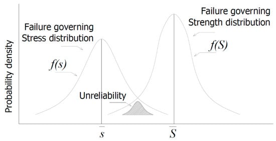
Figure 1.
Stress-strength distribution graphical representation [23].
Therefore, by evaluating Equation (17), the stress/strength reliability and its cumulative failure probability indices are given as
where S is the strength variable and s is the stress variable. Additionally, since we did not observe failure time data in the beam analysis, then the standard deviation for the analysis was determined based on the normal variation coefficient (cv) given as
Since for the normal distribution, the cv value must be , then from Equation (20), the numerical value of the standard deviation used in the beam analysis is given as
Based on the above analysis, the proposed method to determine the element’s reliability is as follows.
3. Proposed Stress-Strength Method
The novelty of the proposed method is that it let us determine the reliability of a structural element based on the time-dependent stress and its corresponding strength as follows.
3.1. Steps to Determine the Stress Distribution
- Step 1.
- For the application case, determine its static properties, perform the corresponding static analysis, and after validating the principal’s critical variables select the corresponding structural element.
- Step 2.
- Based on the performed static analysis, by using the corresponding equation determine the maximum deflection of the bending beam.
- Step 3.
- By using the static analysis, estimate the corresponding normal stress values generated on the weakest area.
- Step 4.
- Determine the corresponding principal stress values (.
- Step 5.
- Define the time-dependent strain and its corresponding time-dependent stress .
- Step 6.
- Define the stress-strain analysis. Then, based on the defined stress-strain values, determine the true stress and the true strain values.
- Step 7.
- Estimate the strain-life curve .
- Step 7.1.
- Based on the log-linear analysis and by considering the determined value as the stress amplitude () at [2,25], define the constant of the amplitude strain-life curve that define the values.
- Step 7.2.
- Based on the determined stress amplitudes to cycles, determine the corresponding maximum and minimum strains ().
- Step 7.3.
- By using the estimated data given in step 7.2, determine the strain and its components elastic and plastic strain amplitudes (), and its corresponding constant value that defines the strain-life curve .
- Step 8.
- Compare the time-dependent strain determined in step 5 with the maximum strain which represents the desired strain at cycles to failure .
- Step 9.
- By using the estimated equivalent stress , determine its corresponding normal distribution parameters .
To summarize this section, the equivalent stress value and its corresponding stress distribution are both determined. Now the stress-strength analysis can be performed as follows.
3.2. Stress-Strength Analysis
Based on the normal strength distribution function and on the normal stress distribution function , the standardized normal Z value utilized to determine the corresponding reliability, can be determined as follows.
- Step 10.
- For the selected material, determine its principal strength values and determine its corresponding normal distribution parameters .
- Step 11.
- By using Equation (17), determine the Z value.
- Step 12.
- Take the probability that the Z value estimated in step 11 represents the reliability index of the analyzed element.
The following section presents the application of the proposed method.
3.3. Numerical Application of the Proposed Method
The objective of this section is to perform the stress-strength analysis for a given structural element by using the normal distribution approach. Thus, as an application case, the left end fixed-right end free and uniformly loaded W beam is performed by using the LRFD method [6]. With this data, following the proposed method, the step-by-step analysis is as follows.
3.3.1. Stress Distribution Based on the Time-Dependent Stress
- Step 1.
- In this case, the beam is supposed to be continuously braced, and for the analysis, the variables are the clear length 9.00 m, and the uniform load 49.25 kN/m. The selected beam is the W33X291, and in the analysis, its weight was added. Now, based on Figure 2, the reaction force at point A is 443.22 kN.
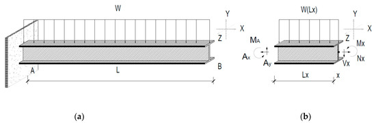 Figure 2. Static/elastic analysis: (a) Left end fixed-right end free and uniformly loaded W beam; (b) Loads, shear forces, and bending moments for a given cross-section.
As the flexural members are subjected to fatigue, by using the static analysis for beams, the maximum bending moment at point A is 1994.50 kN⋅m. Using the static analysis values, the required inertia moment 18,222.33 was compared against the selected W33X291 beam inertia moment 17,700 . Additionally, the principal variables to validate the selected W beam were the AASHTO normative, from which the generated beam deflection should not be higher than , and the design specification for flexural members as per the LRFD method [6]. Thus, the deflection analysis is given next.
- Step 2.
- Based on the application case, the deflection of the bending beam is determined as
By using the estimated values in step 1 of Equation (23) with 18,222.33 , the maximum deflection for the beam is 0.0227 m. Thus, based on the AISC design of flexural members [6] and the W beam weight-cost criterion, the selected beam is considered to be right.
Now, let us determine the generated normal stress values that are acting on the cross-sectional area as follows.
- Step 3.
- For the application case, the formulated analysis for the normal and shear stresses are
From Equation (25), the normal stress value is 105.74 MPa; from Equation (26), the normal stress value is 67.47 MPa [26]; from Equation (27), the shear stress value is 1.93 MPa.
- Step 4.
- Based on data from step 3, from Equation (5), 86.60 MPa; from Equation (2), 105.84 MPa; from Equation (3), 67.37 MPa, and; from Equation (4), 19.23 MPa.
As a summary of the previous analysis and based on the 98% safety factor given on the LRFD method for design [5,6], the W33X291 beam is selected to be analyzed by using the viscoelastic approach. However, due to the addressed principal stress value being static, let us now, based on the linear viscoelastic approach, determine it depending on time as .
- Step 5.
- By incorporating the value of the maximum principal stress as in Equation (8), the effect of the elastic modulus through time is determined. Similarly, by using the time-dependent elastic modulus () values in Equation (13), the corresponding time-dependent stress value is determined. In Equation (8), the used viscoelastic parameter was 9.5 × 10¹⁰ GPa⋅s, which according with Sun et al. [16] corresponds to 20 . The corresponding analysis is given in the Table 2.
Table 2. Time-dependent stress data.
In Table 2, elastic modulus is given in GPa, time is measured in seconds s, the corresponding deflections are given in meters , and the strain values are dimensionless.
Because the changes of the deflections generate the internal bending moment to change, then for any , by performing the static analysis the corresponding must be estimated and utilized to determine its equivalent value (See Equation (32)). In Table 2, the value that corresponds to is also given.
Moreover, because the strain determines the equivalent stress , then the maximum strain that corresponds to is needed. Based on this, let us develop the numerical application.
- Step 6.
- Based on Arasaratnam et al. [20], the data for the stress-strain analysis is shown in Table 3.
Table 3. Data of the selected structural element.
In Table 3, the strain values are dimensionless and the stress data is given MPa.
After this analysis, the stress-strain behavior of the material was determined. But, due to the analysis of the main cycles is performed at , then the strain-life curve is given next.
- Step 7.
- Based on the true stress-true strain values given in Table 3, the strain-life curve analysis is as follows.
- Step 7.1.
- Based on the true stress-true strain values, the stress amplitude and the constant b value are determined as follows:
By taking at , and by considering that [2,25], from Equation (28), the constant b value is given as:
Consequently, , and by substituting it into Equation (28), the stress amplitudes values are shown in Table 4.
Table 4.
Strain-life curve data.
In Table 4, the strain values are dimensionless and the stress data is given MPa.
- Step 7.2.
- By using the values and by taking the minimum stress , the estimated values of the maximum and minimum strain () that define the hysteresis loops given in Figure 3 are:
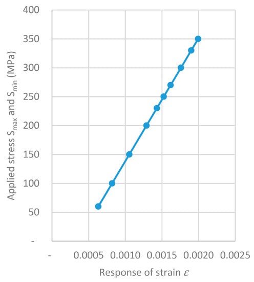 Figure 3. Hysteresis loop of the stress amplitude. Note: Notice that hysteresis loops analysis of Table 4 for each row is needed.
As a result, by using data obtained in step 7.2, the determined values of the strain amplitude are shown in Table 4. Here it is important to highlight that the value of the determined for is related to the determined time-dependent strain value that defines the equivalent stress in step 5.
- Step 7.3.
- By using both the plastic strain amplitude data and the defined cycles to failure values, the log-linear analysis constant c value is 0.3643. The generated strain-life curve is shown in Figure 4.
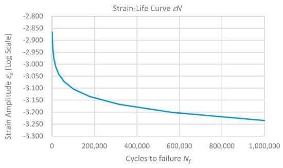 Figure 4. curve.
- Step 8.
- As the objective is to define the cycles to failure that correspond with the strain of 0.000864, then the determined value of the strain given in Table 2 of step 5 0.000864 was interpolated. To this interpolated value, the corresponding time-dependent stress, as shown in Table 2 is 74.28 MPa. Nevertheless, because the time-dependent stress represents the generated maximum principal stress at , then the equivalent supposed load that generates the determined deflection at this time can be estimated as
By using this value, the corresponding equivalent stress is 184.03 MPa. The main goal of this section is to estimate the stress distribution by using the determined equivalent stress , therefore, the next normal distribution analysis is also necessary.
- Step 9.
- By using the equivalent stress 184.03 MPa value as a mean of the normal distribution and its estimated standard deviation 18.40 value, the normal stress distribution parameters are (184.03, 18.40).
Now, the strength distribution analysis is given.
3.3.2. Stress-Strength Analysis
The steps to determine the normal distribution parameters of the strength are as follows:
- Step 10.
- By using the tensile strength = 119.89 MPa value as the mean of the normal distribution and its estimated standard deviation 11.98 value, the normal strength distribution parameters are (119.89, 11.98).
- Step 11.
- Based on the stress (184.03, 18.40) and the strength (119.89, 11.98) distributions parameters, from Equation (17), −0.0013.
- Step 12.
- From the Z value, the reliability of the stress-strength function for the W beam 33X291, is R(t) = 1%.
In Table 5, the weigh-cost analysis for the W beams 30X357 and 33X318 is given.
Table 5.
Selected structural elements based on the proposed stress-strength method.
Consequently, as a result of the application case given in Section 3.3, from the second column of Table 5, the W beam weight-cost that better fulfills the LRFD and AISC selection methods is the W33X291. Note that even though the performance of the W beam W30X357 fulfills the LRFD and AISC methodologies, among the three alternatives is the one that presents higher reliability. Therefore, designers can select the one that they consider the best choice for their objective. In our case, we recommend the beam with higher reliability. Finally, notice when we use less modified factors the designed reliability will be higher, this because the higher the value, the higher the reliability.
4. Conclusions
- (1)
- Because the generated internal stresses are always related to the bending beam, and since the proposed method uses these stress values to determine the stress distribution, then the reliability of any structural element can always be determined by applying the proposed method.
- (2)
- Because the applied stresses are independent of the material strength, then the proposed method can be used as a complement to the classic design methodology of structural elements based on the reliability index to discriminate among the possible addressed alternatives.
- (3)
- Because the proposed method can be performed for any desired cycles, from the element selection to the reliability determination, then it can be used as a guideline in any structural analysis. Although here the analysis was performed at 106 cycles (or at the value), it can be performed at any desired cycles.
- (4)
- Note that as in Table 5, when the value is lower than the expected equivalent stress , then both the plastic and fracture of cracked mechanical components analysis should be performed.
- (5)
- Note because the less used modified factors the higher the value, then for environments where fewer modifier factors are needed, the designed beam reliability index will be higher.
- (6)
- As the principal stress values on which the proposed method is based are the eigenvalues of a quadratic form represented by the stress matrix, the proposed method can be used to determine the reliability of an analyzed element in any field where the eigenvalues are known. As is the case for a principal components analysis and a quality analysis where they are performed using a second-order polynomial model.
Author Contributions
Conceptualization, A.M., M.R.P.-M., S.T.d.l.C.-C., J.M.B.-C.; methodology, A.M., M.R.P.-M.; data analysis, A.M., S.T.d.l.C.-C.; writing-original draft preparation, A.M., M.R.P.-M.; writing-review and editing, A.M., M.R.P.-M., S.T.d.l.C.-C., J.M.B.-C.; supervision, M.R.P.-M.; funding acquisition, A.M., M.R.P.-M. All authors have read and agreed to the published version of the manuscript.
Funding
This research received no external funding.
Institutional Review Board Statement
Not applicable.
Informed Consent Statement
Not applicable.
Data Availability Statement
Not applicable.
Conflicts of Interest
The authors declare no conflict of interest.
References
- Brinson, H.F.; Brinson, L.C. Polymer Engineering Science and Viscoelasticity: An Introduction; Springer: Boston, MA, USA, 2008. [Google Scholar]
- Dowling, N.E. Mechanical Behavior of Materials: Engineering Methods for Deformation, Fracture, and Fatigue; Pearson: Boston, MA, USA, 2013. [Google Scholar]
- Weibull, W. A Statistical Theory of Strength of Materials. In Generalstabens Lotografiska Anstalts Förlag; Centraltrycheriet: Stockholm, Sweden, 1939; pp. 5–10. [Google Scholar]
- Duffy, S.F.; Gyekenyesi, J.P. Time Dependent Reliability Model Incorporating Continuum Damage Mechanics for High-Temperature Ceramics. NTRS. 1989. Available online: https://ntrs.nasa.gov/citations/19890015116 (accessed on 9 April 2021).
- McCormac, J. Diseño de Estructuras de Acero; Alfaomega Grupo Editor S.A. de C.V.: Mexico City, Mexico, 2016. [Google Scholar]
- Design, A.S. Specification for Structural Steel Buildings; AISC: Chicago, IL, USA, December 1999; Volume 27. [Google Scholar]
- Zadeh, H.J.; Nanni, A. Reliability Analysis of Concrete Beams Internally Reinforced with Fiber-Reinforced Polymer Bars. Struct. J. 2013, 110, 1023–1032. [Google Scholar]
- Baji, H.; Ronagh, H.R. Reliability-Based Study on Ductility Measures of Reinforced Concrete Beams in ACI 318. Struct. J. 2016, 113, 373. [Google Scholar] [CrossRef]
- Xue, W.; Peng, F.; Xue, W. Reliability-Based Design Provisions for Flexural Strength of Fiber-Reinforced Polymer Prestressed Concrete Bridge Girders. Struct. J. 2020, 116, 04020086. [Google Scholar]
- Eryilmaz, S. On Stress-Strength Reliability with a Time-Dependent Strength. J. Qual. Reliab. Eng. 2013, 2013, 1–6. [Google Scholar] [CrossRef]
- Piña-Monarrez, M.R. Weibull stress distribution for static mechanical stress and its stress/strength analysis. Qual. Reliab. Eng. Int. 2017, 34, 229–244. [Google Scholar] [CrossRef]
- Barraza-Contreras, J.M.; Piña-Monarrez, M.R.; Molina, A. Fatigue-Life Prediction of Mechanical Element by Using the Weibull Distribution. Appl. Sci. 2020, 10, 6384. [Google Scholar] [CrossRef]
- Alrubaie, M.A.A.; Gardner, D.J.; Lopez-Anido, R.A. Modeling the Long-Term Deformation of a Geodesic Spherical Frame Structure Made from Wood Plastic Composite Lumber. Appl. Sci. 2020, 10, 5017. [Google Scholar] [CrossRef]
- Asyraf, M.; Ishak, M.; Sapuan, S.; Yidris, N. Influence of Additional Bracing Arms as Reinforcement Members in Wooden Timber Cross-Arms on Their Long-Term Creep Responses and Properties. Appl. Sci. 2021, 11, 2061. [Google Scholar] [CrossRef]
- Wang, B.; Huang, W.; Zheng, S. Study on Restoring Force Performance of Corrosion Damage Steel Frame Beams under Acid Atmosphere. Appl. Sci. 2018, 9, 103. [Google Scholar] [CrossRef]
- Sun, Y.; Maciejewski, K.; Ghonem, H. Simulation of Viscoplastic Deformation of Low Carbon Steel Structures at Elevated Temperatures. J. Mater. Eng. Perform. 2011, 21, 1151–1159. [Google Scholar] [CrossRef][Green Version]
- Gere, J.M.; Timoshenko, S. Mechanics of Materials; Brooks/Cole: Pacific Grove, CA, USA, 2001; pp. 815–839. [Google Scholar]
- Timoshenko, S. Resistencia de Materiales, Segunda Parte; Espasa-Calpe Sa: Madrid, Spain, 1957. [Google Scholar]
- Ugural, A.C.; Fenster, S.K. Advanced Mechanics of Materials and Applied Elasticity, 5th ed; Prentice Hall: Englewood Cliffs, NJ, USA, 2011. [Google Scholar]
- Arasaratnam, P.; Sivakumaran, K.S.; Tait, M.J. True Stress-True Strain Models for Structural Steel Elements. ISRN Civ. Eng. 2011, 656401. [Google Scholar] [CrossRef]
- Budynas, R.G.; Nisbett, J.K. Shigley’s Mechanical Engineering Design; McGraw-Hill: New York, NY, USA, 2008; Volume 8. [Google Scholar]
- Lee, Y.-L.; Pan, J.; Hathaway, R.; Barkey, M. Fatigue Testing and Analysis: Theory and Practice; Elsevier Butterworth-Heinemann: Burlington, MA, USA, 2005; Volume 13. [Google Scholar]
- Kececioglu, D. Robust Engineering Design-by-Reliability with Emphasis on Mechanical Components & Structural Reliability; DEStech Publications, Inc.: Pennsylvania, PA, USA, 2003. [Google Scholar]
- Baro, M.; Monarrez, M.R.P.; Villa, B. Stress-Strength Weibull Analysis with Different Shape Parameter β and Probabilistic Safety Factor. Dyna 2020, 87, 28–33. [Google Scholar] [CrossRef]
- Zhang, J.; Li, W.; Dai, H.; Liu, N.; Lin, J. Study on the Elastic–Plastic Correlation of Low-Cycle Fatigue for Variable Asymmetric Loadings. Materials 2020, 13, 2451. [Google Scholar] [CrossRef] [PubMed]
- Molina, A.; Piña-Monarrez, M.R.; de la Cruz-Cháidez, S.T. Análisis metodológico del esfuerzo normal σyy basado en deflexión elástica. Rev. Ciencias Tecnológicas 2019, 2, 166–180. [Google Scholar] [CrossRef]
Publisher’s Note: MDPI stays neutral with regard to jurisdictional claims in published maps and institutional affiliations. |
© 2021 by the authors. Licensee MDPI, Basel, Switzerland. This article is an open access article distributed under the terms and conditions of the Creative Commons Attribution (CC BY) license (https://creativecommons.org/licenses/by/4.0/).