1. Introduction
The most popular vector spatial operations like overlay or intersections of geometries, areas of influence (buffer operator), etc. require calculations that are made up of other basic geometric calculations such as:
Operation A: Distance and azimuth (bearing) between two points.
Operation B: Calculation of a second point, from a starting point, an azimuth and a distance.
Operation C: Area calculation.
Operation D: Line intersection.
Operation E: Minimum distance from a point to a line.
Any spatial analysis software implements these basic geometric calculations in 2D/3D by itself or through some computational geometry libraries like GDAL, JTS, etc. [
1]. The geometry calculations are performed with Cartesian coordinates using Euclidean (flat) geometry. However, it is well-known that the Earth’s standard reference surface is the ellipsoid (or spheroid, as it is occasionally named), as regards planimetric operations, and the geoid for the case of the vertical component [
2]. Ellipsoids are geometrically defined by two parameters, usually the flattening
f and major semiaxis
a [
3]. Different values for these defining geometrical parameters can be found in the different reference ellipsoids that have been historically proposed, to name a few:
a = 6,378,206 m and
f = 1/294.98 for Clarke 1866 [
4],
a = 6,378,249.145 m and
f = 1/293.465 for Clarke 1880 [
5],
a = 6,378,388 m and
f = 1/297 for Hayford [
3],
a = 6,378,137 m and
f = 1/298.257222101 for GRS80 [
6] and
a = 6,378,137 m and
f = 1/298.257223563 for WGS84 ellipsoid [
5], whose minuscule discrepancy with respect to the GRS80 of 0.1 mm in the direction of the minor semiaxes is negligible for all practical purposes.
The reference ellipsoid also needs to be assigned a mass and angular velocity, which are conventionally adopted, for it to serve as a dynamic reference. Further, the ellipsoid needs to be conveniently placed with respect to the Earth’s center of mass or geocenter, so that a global geodetic reference system is obtained. The realization (or practical implementation) of the reference system is done by means of a set of geodetic benchmarks with coordinates assigned after complex calculations involving different geodetic techniques (Satellite Laser Ranging, Very Long Baseline Interferometry, Global Navigation Satellite Systems and Doppler Orbitography and Radiopositioning Integrated by Satellite [
7]).
This has eventually resulted in the proposal of the International Terrestrial Reference System (ITRS) and its most recent realization, the International Terrestrial Reference Frame 2014 (ITRF2014 [
7]), as the most accurate scientific reference for geospatial analysis [
8]. The subsequent realizations of the WGS84 reference system (used by the GPS constellation since its initial deployment), have been increasing aligned with the realizations of the International Terrestrial Reference System so that the latest ones, WGS84(G1762) and ITRF2014, are equivalent in practice (they are consistent at the centimeter level [
9,
10,
11]). The practical equivalence of both the WGS84 ellipsoid and the WGS84 reference system with the GRS80 ellipsoid and the ITRS is therefore implied in the rest of the paper.
However, solving a geometric problem on the surface of the ellipsoid is not a simple task. Therefore, the auxiliary use of map projections is normally preferred. By means of local projections, the geographic coordinates (on a reference ellipsoid) are converted to flat coordinates and thus all the above calculations can be easily applied.
Any geometric calculation using map projections must take into account that the particular type of projection and defining parameters [
12] entail several limitations, chiefly:
a limited, non-universal, area of use;
scale distortions, leading to different scale factors for different points in the area;
angle distortions: even for the case of conformal projections, that is those preserving angles, the angle preservation at every point A is fulfilled between the tangents to the original geodetic lines on the ellipsoid at A and the tangents to the projected lines at A, which are not straight lines on the map but curved lines. If the straight segments, or chords, joining line ends are considered, the original angle is not preserved;
area distortions: even for the case of equal-area projections, the area of figures enclosed by geodetic lines is not preserved as the area in the map enclosed by the straight segments connecting the extreme points.
Hence, there is no projection that helps to accurately solve the geometric calculations for a large area.
In recent years, the most powerful spatial analysis software solutions (Oracle, Google Earth Engine, PostgreSQL + PostGIS, etc.) have implemented some geometric calculations directly on the spheroid. In this way, these software can offer high accuracy over large areas (countries or even continents).
Operations A and B above can be accurately calculated on the ellipsoid. They are known as the direct and inverse problems of geodesy and allow the calculation of distances and angles (azimuths) between two points on the ellipsoid. The calculation involves numerical integrations and an iterative approach. There is a large number of algorithms both efficient and accurate, even considering long distances, which provide an accuracy close to the machine precision, such as GeographicLib [
13,
14], since the idea that the software tools developed should provide the user with the highest possible accuracy (close to machine precision) has become more and more prevalent in recent times.
For more than a decade now, the geospatial analysis software products (GIS Desktop, Spatial Databases, and computational geometric libraries) have incorporated quite good implementations on the ellipsoid of operations A and B with high accuracy (e.g., the methods ST_Azimuth, ST_Project and ST_Distance in PostGIS [
15]). More recently even the operation C has been addressed [
16,
17].
The problem appears with the operations D and E. Currently very few products implement these operations on the ellipsoid and the calculations are not performed precisely but roughly (the errors depending on the distance and the software used can easily reach meters). We will demonstrate this in the next section. To do so, an algorithm introduced by the authors in a previous article [
18] for solving operation E, has needed to be improved.
The main goals of this research are:
To test the current geospatial solutions and check that they give approximate results when talking about ellipsoid calculations.
To present two new algorithms to solve operations D and E accurately in a spatial database (PL/SQL) and with Java as a library, so that anyone can easily use it.
To verify the results of the proposed algorithms (within the desired accuracy of 100 nm).
To encourage the spatial analysis software vendors to implement the algorithms on the ellipsoid so that accurate results can be achieved.
2. Experiments
Our hypothesis states that some of the most powerful geospatial software products provide only approximate results in the calculations of operations D and E on the ellipsoid, despite that, some software companies claim that these calculations are accurate.
We start with operation D, first describing the methodology used by each software and then demonstrating how the results of the calculations are in all cases approximate. Operation E is discussed in
Section 4.3.
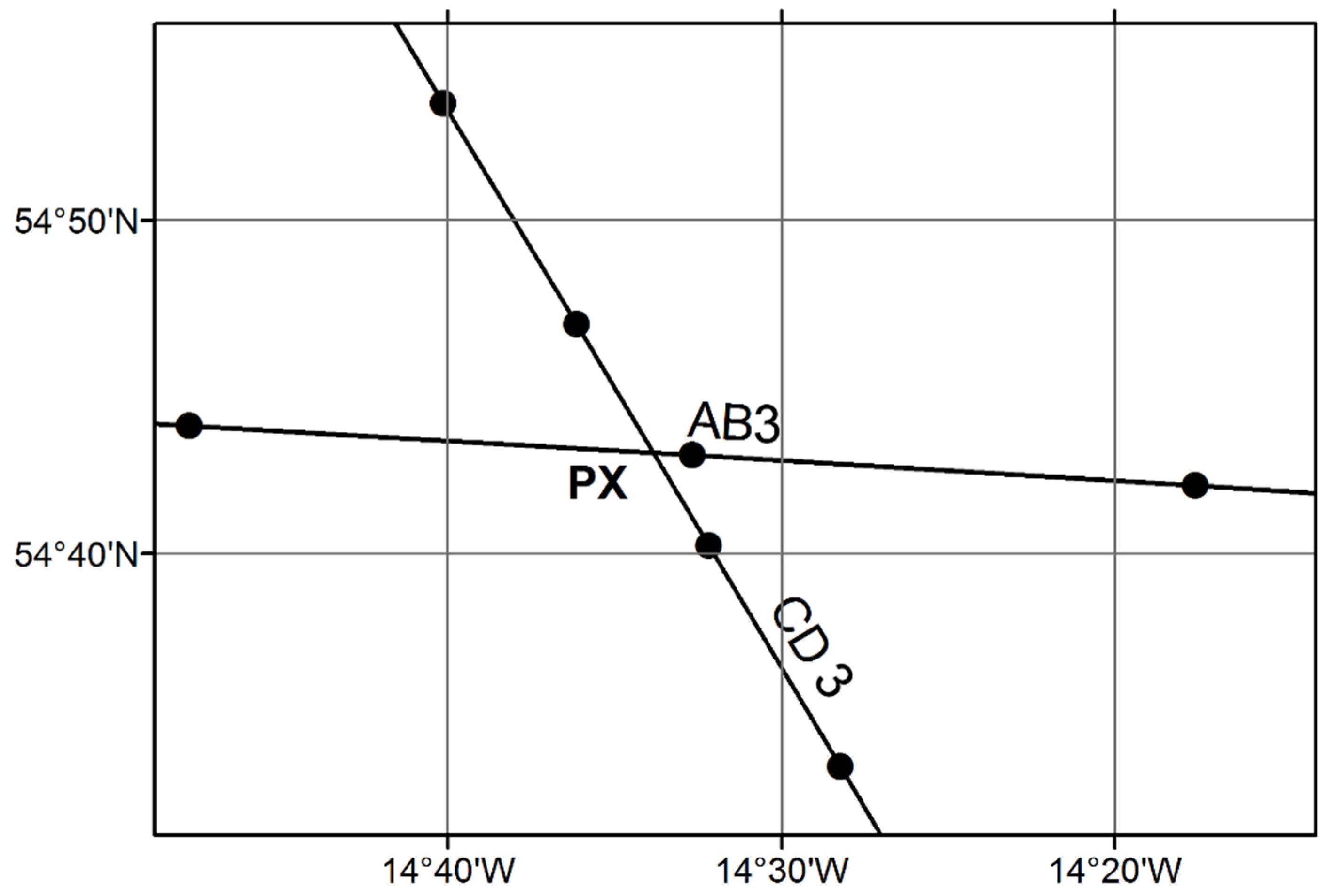
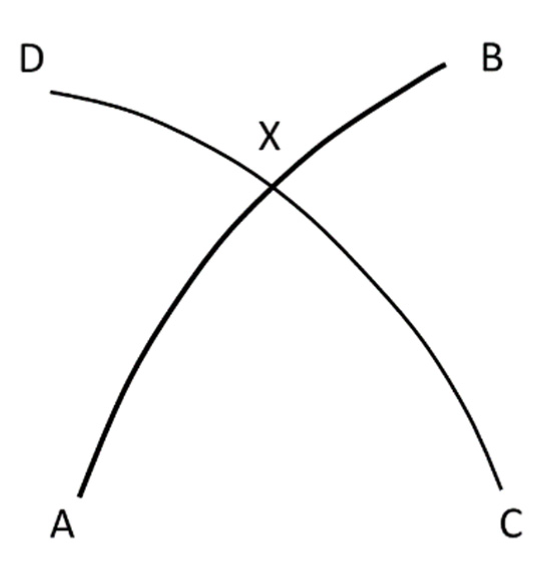
For all the examples the ellipsoid WGS84 is used. First, we will solve a simple intersection of two geodesics defined by four points. Given points A, B, C and D on the ellipsoid (
Figure 1) we calculate the intersection (denoted by X) of geodesics AB and CD with different software products.
In
Table 1 four cases are distinguished for short, medium, long and very long lines, depending on the coordinates given for A(
φA,
λA), B(
φB,
λB), C(
φC,
λC) and D(
φD,
λD): Case 1 A(54.0°,14.5°), B(54.2°,14.6°), C(54.1°,14.4°), D(54.0°,14.7°), distances AX and CX are 6.6 and 9.6 km; Case 2 A(52°,5°), B(51.4°,6°), C(51.5°,4.5°), D(52°,5.5°), distances AX and CX are 21.6 and 64.7 km; Case 3 A(42°,29°), B(39°,−77°), C(6°,0°), D(64°,−22°), distances AX and CX are 345 and 556 km; Case 4 A(35°,−92°), B(40°,52°), C(−8°,20°), D(49°,−95°), distances AX and CX are 2003 and 11,347 km. In the first example, the distance (average of AX and CX) is 8 km. For the second, third and fourth examples, the distances are 43, 450 and 6675 km, respectively. For each of the three geospatial software groups, namely geographic information systems (GIS), spatial database management systems (SDBMS) and geospatial libraries (APIs), we chose one of the most powerful solutions. Representing the first group, we will test ArcGIS by ESRI [
19], which is a very well-known and powerful GIS Desktop solution, spread all over the world and used by many public governments. It is worth noting that none of the open-source GIS desktops (QGIS, GRASS, gvSIG, uDIG, etc.) implement operations D or E on the ellipsoid. The best known and most advanced open-source Spatial DBMS is, definitely, PostGIS [
20] but it is discarded because it does not implement the D or E operations on the ellipsoid. We will use instead one of the most powerful spatial DBMS commercial solutions: the Oracle Spatial extension [
21], which allows us to solve operations D and E on the ellipsoid. Regarding geospatial libraries using the ellipsoid in their algorithms we can find Google Earth Engine [
22], which is one of the most powerful Geospatial API solutions, with many new features in recent years.
The last row of
Table 1 shows the geocentric coordinates from the result of intersecting the two great circles AB-CD using a sphere. Solving the intersection is trivial if we consider a sphere instead of an ellipsoid. In that case, the minimum distance between two points on the surface of the sphere is not a geodesic of complicated geometry but a simple great circle (orthodrome). The intersection of two great circles using some spherical trigonometry math is solved by a very straightforward formula [
23] but at the cost of possibly having huge discrepancies with respect to the true intersection on the ellipsoid.
In this section we will prove that some spatial software are using great circles and not geodesics on the ellipsoid. In
Section 3, we design two tests to assess the errors of the different software solutions. In
Section 4, the true intersection on the ellipsoid will be calculated and the designed tests from
Section 3 will demonstrate the high accuracy reached by the proposed algorithm.
2.1. Oracle Spatial
The official documentation mentions that Oracle supports geodetic coordinate systems and says that computation involving large areas or requiring very precise accuracy must account for the curvature of the Earth’s surface [
24]. It also mentions that Oracle provides a rational and complete treatment of geodetic coordinates.
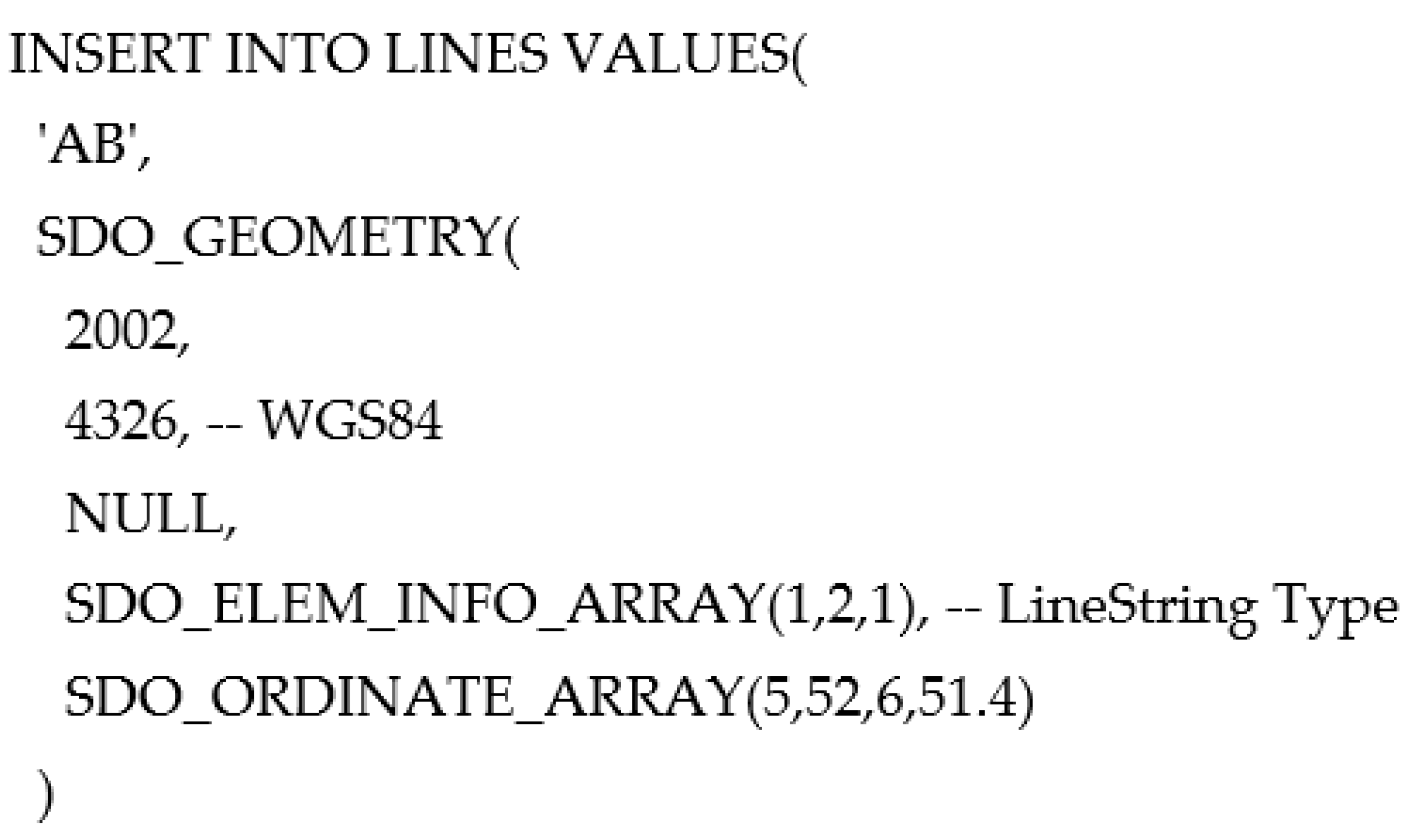
Oracle Spatial uses the spatial SQL operator SDO_GEOM.SDO_INTERSECTION (AB, CD) to intersect two geodesics on the ellipsoid.
Scheme 1 shows how the geodesic AB is defined with the coordinates (SDO_ORDINATE_ARRAY) and the reference system 4326 corresponding to WGS84.
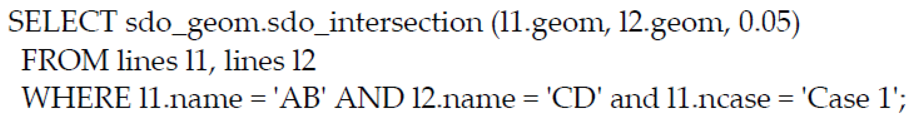
Oracle needs a coordinate tolerance to perform any spatial operation. The command shown in
Scheme 2 intersects the geodesics AB and CD with a tolerance of 0.05 m, which is the smallest tolerance, allowed by Oracle for geodetic calculations. The resulting coordinates for the intersection are shown in
Table 1.
Table 1 shows that the results from Oracle and the results using a sphere (last row) are completely equal. This is enough to assert that Oracle is not using an ellipsoid in its calculations and therefore does not intersect two geodesics on the ellipsoid but two great circles on the sphere. The Oracle SQL code with the four intersection cases and the results can be found in the GitHub repository [
25] (journal_data/geodesicintersection_with_oracle.sql).
2.2. Google Earth Engine
As Google mentions is its own site “Google Earth Engine combines a multi-petabyte catalog of satellite imagery and geospatial datasets with planetary-scale analysis capabilities and makes it available for scientists, researchers, and developers to detect changes, map trends, and quantify differences on the Earth’s Surface” [
26].
It is a powerful platform to run geospatial algorithms. Besides that, the API is available in JavaScript which is really convenient, since you can try it from any modern browser.
Google Earth Engine’s geometry constructors build geodetic geometries by default using the WGS84 ellipsoid [
26]. To make planar geometries (Cartesian coordinates) an additional argument must be specified at the time the geometry is built.
One can use Google Earth Engine API for free after registering. A very easy way to test the API is to use the “Earth Engine Code Editor” which is an online javascript editor ready to use the API.
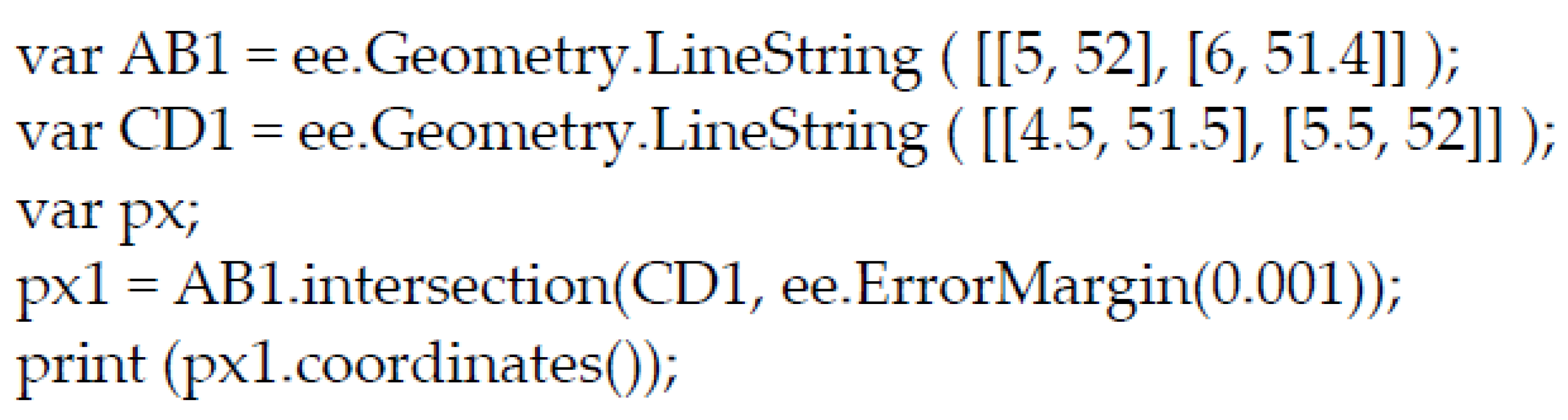
Notice in
Scheme 3 the ErrorMargin function, which specifies a maximum error for geometric operations only in the case of using map projections [
27]. If this value is changed the results remain still. For the first case the source code is.
Table 1 shows that the coordinates obtained from Google Earth and Oracle Spatial are exactly the same. Actually, there is a negligible difference of about 1 × 10
−12 degrees, which represent around 0.3 µm, attributable to machine precision.
It proves that both Google Earth Engine and Oracle Spatial use the same methodology, which consists in using a sphere instead of an ellipsoid.
2.3. ArcGIS
ArcGIS has been chosen as the renowned software representing the GIS Desktop group. ArcGIS Desktop claims that it can create geodetic geometries that are spatially accurate and geodetically correct in any projection, which is especially important when using large distances as airplanes flight paths or effective weapon ranges [
28].
The intersection of the two geodesics can be by calculated through a spatial analysis operation after introducing their coordinates from the graphical interface.
The ArcGIS official documentation [
28] mentions that “Geodetic features contain densified geometry, which is a shape created by a series of connected vertices”, which means that ArcGIS is not using true geodesics either as we will prove in the next section.
For the test, we used a WGS84 dataset, an ArcGIS cluster tolerance and resolution of 0.000001″ (some 0.03 mm) and 0.0000005″ (some 0.015 mm), respectively.
Figure 2 shows a zoom of the intersection zone of geodesics AB-CD (Case 3 in
Table 1) with ArcGIS. It can be seen how ArcGIS is splitting the original line, calculating each of the new vertices on the ellipsoid, but every segment is treated as a straight line (Euclidian geometry) and not a geodesic.
This ArcGIS methodology has two major drawbacks. First, it greatly densifies all the geometries. Each geodesic is divided into thousands of segments (e.g., the geodesic AB from the example 4, is divided into 947 segments), which seriously affects both the performance and the complexity of any spatial operation. Although the segment size used by ArcGIS to split the lines is user-defined, a noticeable improvement in accuracy requires an enormous densification, which is clearly inefficient.
Apart from the computation-expensive densification, the most important drawback is the approximate nature of the process, which uses planar calculations between split segments (Cartesian coordinates instead of geographic coordinates).
2.4. ArcGIS Plus Local Projections
This solution offers a better result than the previous one because it combines the geodetic densification with a local projection. It is not a solution directly built in ArcGIS. It is a user defined process that requires several ArcGIS steps: first, a geodetic densification and then to choose the appropriate projection according to the study area.
As we explained this method does not use calculations on the ellipsoid but local projections with all drawbacks mentioned above (limited area and appearance of distortions including non-straight representation of geodetic lines).
We chose manually the best local projection for each example (e.g., example 4 covers the UTM projection zones from 15 to 42) taking into account that in order to obtain the highest precision, we have to choose the UTM zone that best fits the intersection area (zone 33 for case 1, zone 31 for case 2, 28 for case 3 and 17 for case 4).
Table 1 shows the results provided by ArcGIS using the geodetic densification and calculating the intersection with the Geoprocessing tools [
29] after transforming the data to the best UTM zones. In addition to the drawback of densifying the geometry, using local projections limits the achievable accuracy and the study area.
2.5. PostGIS Plus Local Projections
PostGIS uses Cartesian coordinates to perform operations D and E. PostGIS only uses the ellipsoid to solve operations A, B and C (ST_Azimuth, ST_Distance, ST_Project and ST_Area SQL methods).
We take PostGIS as an example to demonstrate the errors of the spatial analysis tools that follow this methodology. PostGIS determines the best local projection that fits the bounding box of the two geometries (favoring UTM or Lambert Azimuthal Equal Area and falling back on Web Mercator in the worst case scenario). After computing the spatial operation (e.g., intersection, buffering or union) PostGIS project back to WGS84 geographic coordinates [
30].
Table 1 shows the results obtained with PostGIS using this automatic reprojection methodology.
3. Validation of Results
At this point, firstly we must prove in a quantitative way that the coordinates shown in
Table 1 are approximate and do not define the true intersection of two geodesics. Then, in
Section 4, the new proposed algorithm is presented, and we will assess its error with this same quantitative methodology.
We can check the correctness by means of the direct and inverse problems of geodesy. Sjöberg [
31,
32,
33] deals with the problem directly on the ellipsoid by using numerical integration and there are some libraries like the GeographicLib suite [
13] which is optimized to deliver accuracy close to machine precision.
Some of the spatial databases like Oracle Spatial or PostGIS implement the direct and inverse geodesy problems and expose them through SQL functions. All these solutions make these calculations with high precision and yield identical results.
For this test, we only need a library or software that can solve the direct and inverse problems of geodesy. Of the many available solutions, we used the GeographicLib library through PostGIS [
20] (PostGIS Geography Support Functions functions ST_Azimuth and ST_Distance for the inverse problem, and ST_Project for the direct problem). We also tested GeographicLib with a Java implementation that provides the same results.
3.1. Tests
In order to check the geodesic intersection algorithms in a quantitative way we designed two tests to show the deviation in azimuth (Test A) and distance (Test B).
3.1.1. Test A
We can check the accuracy of the intersection of geodesics AB-CD, point X, by inspecting the azimuth equalities: α
AX = α
AB and α
CX = α
CD. The column deviation of
Table 2 shows the value in arcseconds of Test A, Maximum (|α
AX − α
AB|, |α
CX − α
CD|), therefore, any value greater than zero means that point X does not lie on the geodesics exactly.
3.1.2. Test B
As explained below, this test provides a linear magnitude of deviation from the intersection point X to both geodesics AB and CD. It has a clear geometric meaning easily interpretable by the user, in contrast to the previous test.
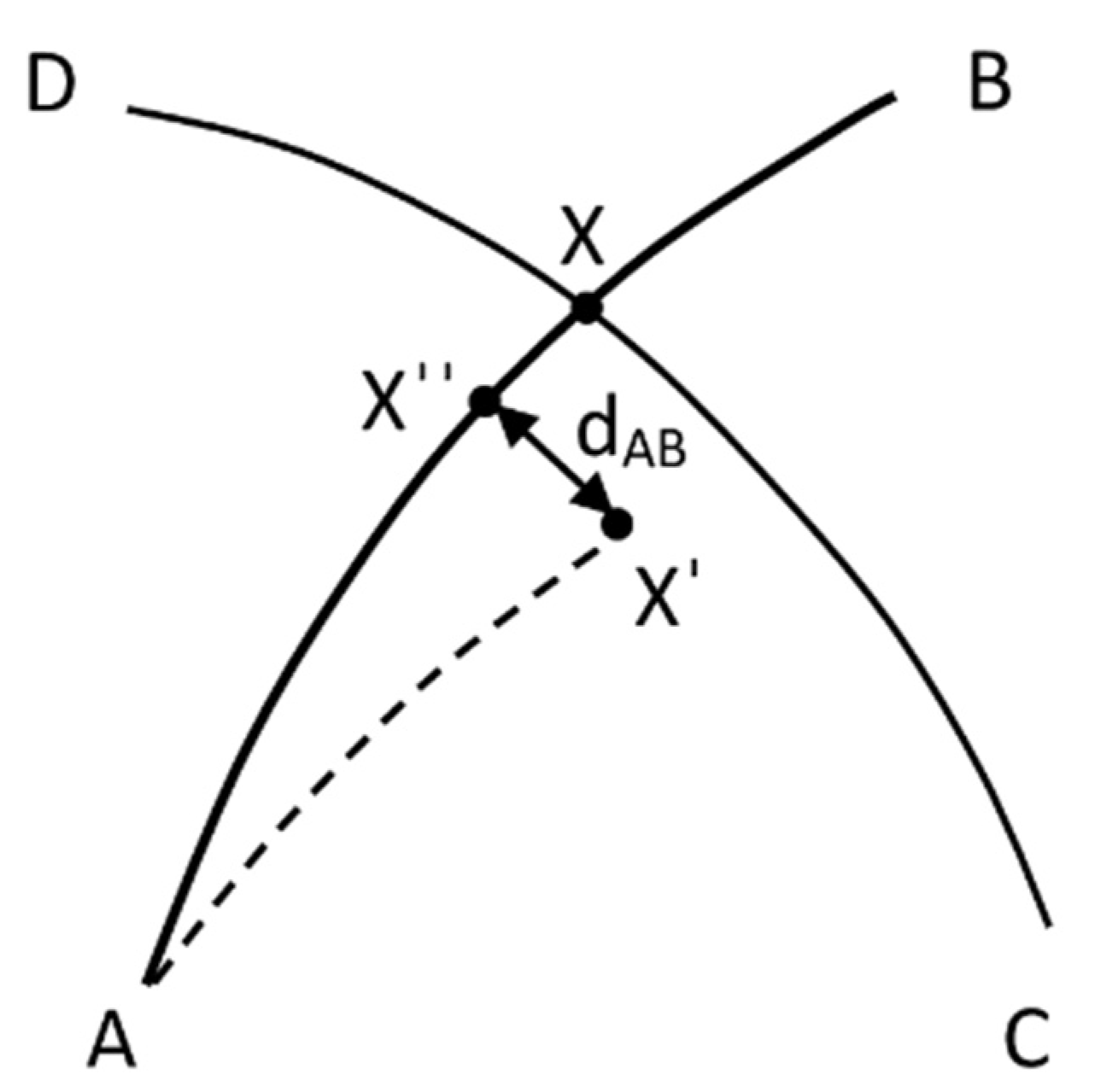
Assume the calculated intersection point X has some error, then the intersection point would be located at X′ instead of X. If so, there would be some deviation d
AB (
Figure 3), between X′ and X″, greater than zero, where X″ is the projection of X′ on the geodesic AB.
From a starting point A, an azimuth αAB and a distance AX′ we can easily calculate X″ through the direct problem of geodesy.
The distance dAB is the distance from the calculated point X′ to the geodesic AB. The same distance can be calculated from the point X′ the other geodesic CD and thus obtain a second deviation distance dCD. If both distances are zero, the X′ point is the exact intersection of the geodesics AB and CD.
The column deviation of
Table 2 shows the value in meters of Test B, Maximum (d
AB, d
CD). The calculation is approximate (although quite accurate as it will be demonstrated in next section) because, obviously, we still do not know where the true point of the intersection is.
As it can be seen in
Table 2, Google Earth Engine and Oracle Spatial show a deviation (test B) of almost 5 km. This is due to the computing with the sphere instead of the ellipsoid. ArcGIS, even in the case of using local projections after applying a densified geodesic, shows deviations of several tens of meters.
Additionally, PostGIS, with its spatial operators (which internally use local reprojections) shows a deviation of several meters in case 2. Cases 3 and 4 should not count too much, since PostGIS in these cases uses the Web Mercator projection that introduces huge deformations. Hopefully PostGIS will improve the choice of the best projection for these cases, which would limit the deviation to hundreds of meters.
The most favorable example, case 1, shows a deviation of several centimeters, an amount that, according to the purpose of the spatial analysis, could already be intolerable.
4. Exact Solution and Validation
This section presents the implementation of the algorithms designed by the authors of this paper for operations D and E on the ellipsoid by means of highly accurate fast-convergent iterative algorithms which were initially presented in [
18]. As explained later, however, the iterative algorithm for operation E has been improved for the purpose of a better and even faster convergence to the exact solution.
We made two different implementations of the algorithm: in Java, creating a library (API) that allows the user to integrate it with their own applications, and in PL/SQL (SQL stored procedures) with a PostGIS spatial DBMS. With PostGIS, a GIS user can take advantage of all the spatial functionality and run the geodesic intersections with its own cartography easily.
Both implementations can be found in a public repository [
25], files src/GeodesicSpatialOp.java and src/GeodesicSpatialOp.sql.
For the implementation of the algorithm, we need to call some functions to get the inverse and direct solutions of geodesics on the ellipsoid. Any algorithm that gives a high accuracy (100 nm or more) can be used. We chose Karney’s implementation [
13], due to its accuracy, robustness and a wide range of supporting programming languages. The numeric precision for floating types is 64 bits, which is supported by PostgreSQL or Java.
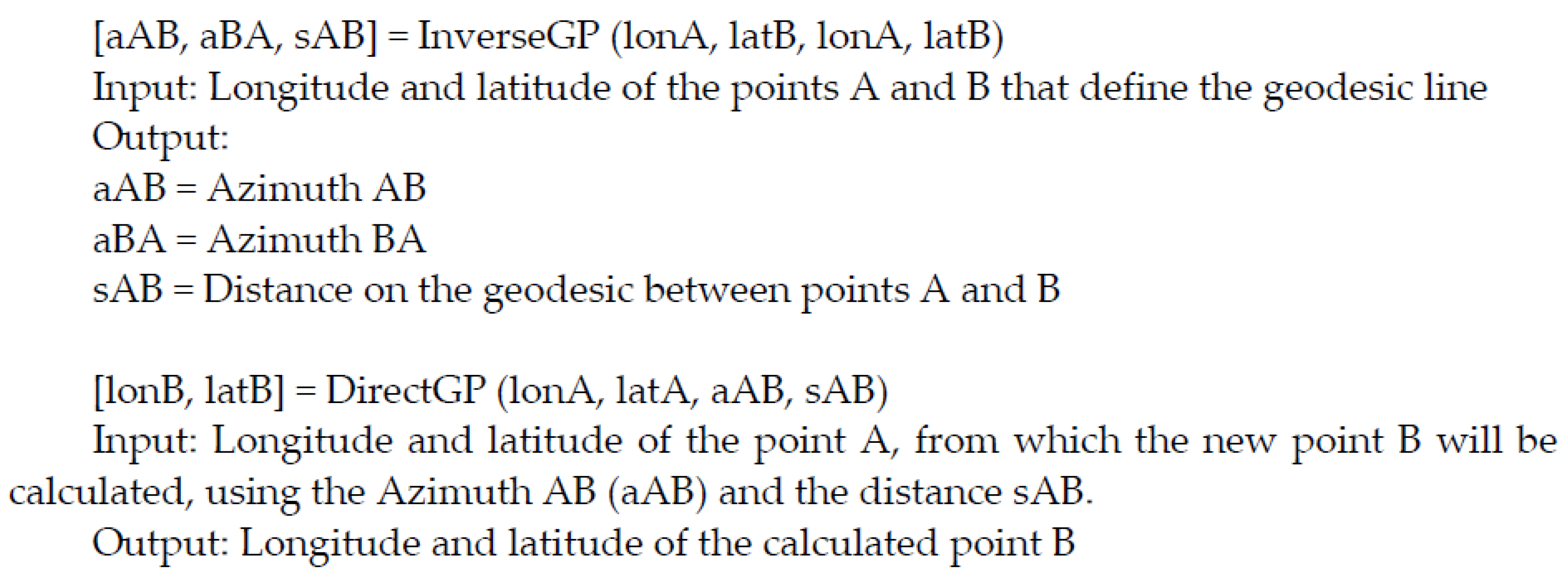
Scheme 4 shows the inputs and outputs of the functions InverseGP and DirectGP that solve the inverse and direct geodesic problem. All azimuths and coordinates are in radians. Both functions are working with WGS84.
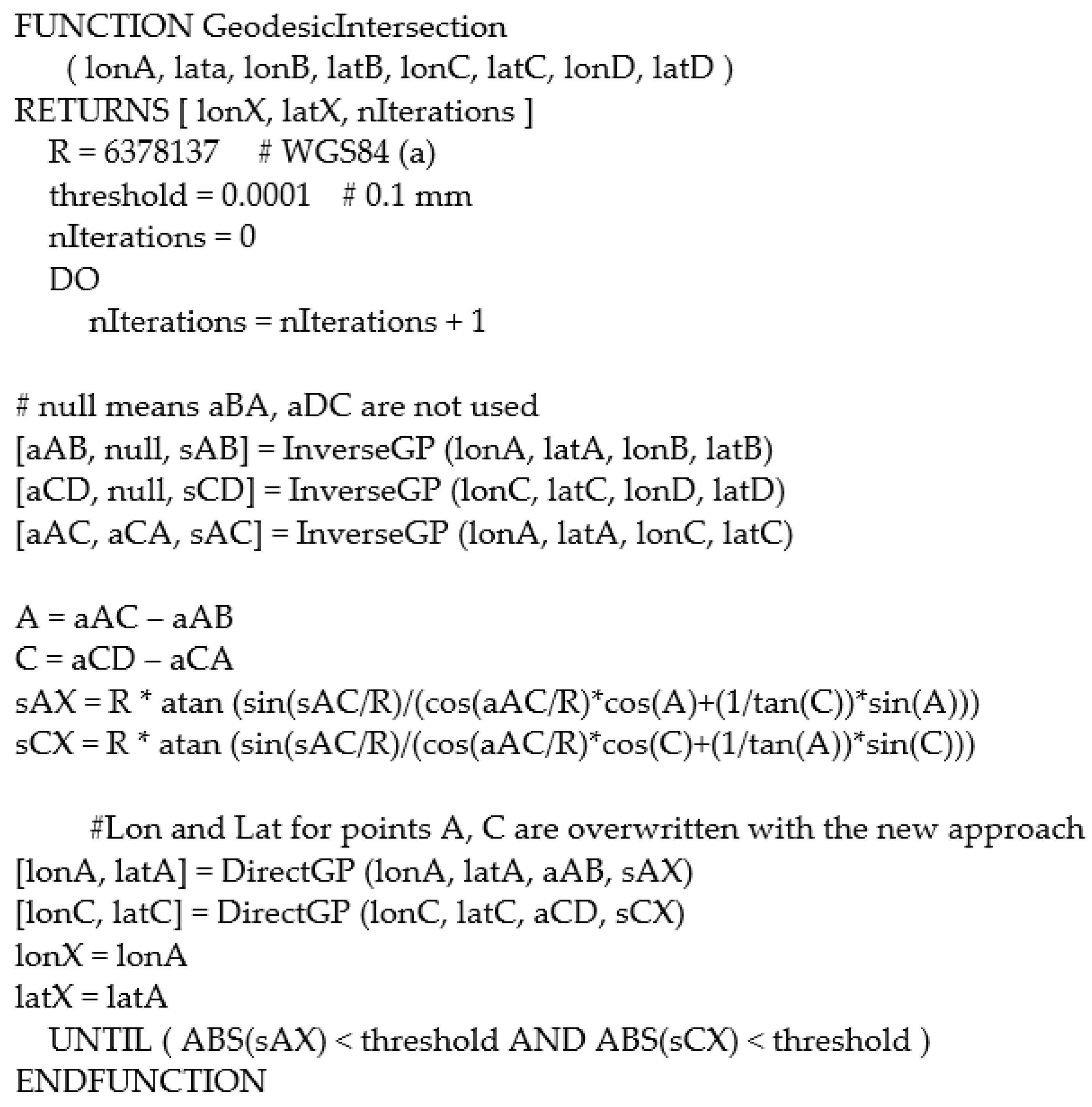
Scheme 5 shows the pseudocode of the Geodesic Intersection algorithm which returns the longitude and latitude of the intersection point X, and the number of iterations needed. Comments are denoted by #.
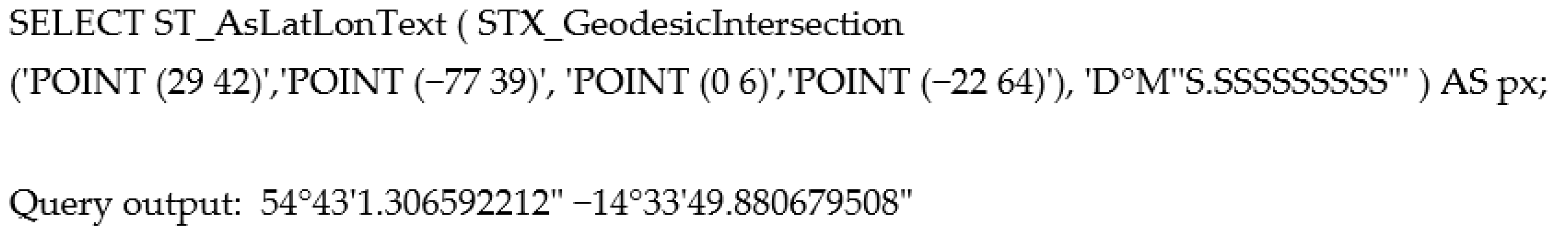
The new spatial PostGIS SQL function “STX_GeodesicIntersection (a point, b point, c point, c point)” calculates the intersection of the two geodesics AB-CD on the ellipsoid WGS84 (ellipsoid by default).
Scheme 6 shows how a SQL user can easily get the intersection of two geodesics.
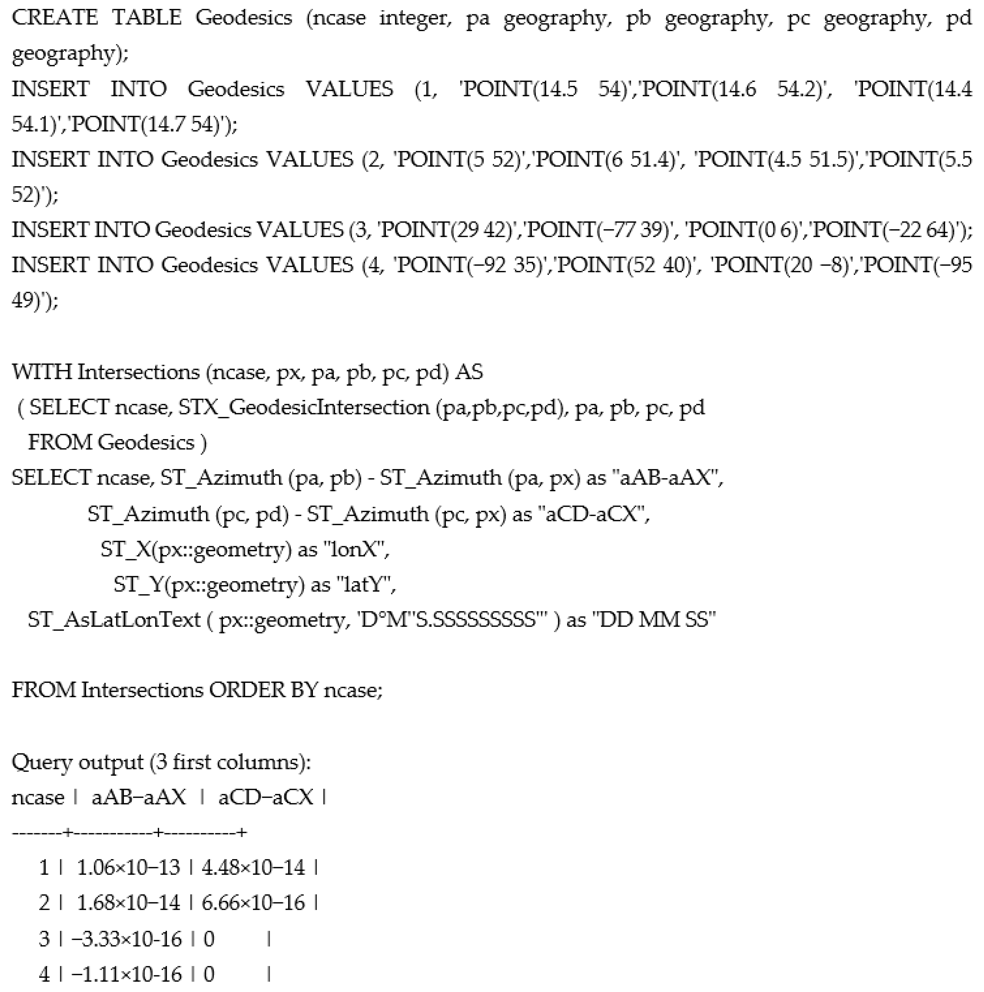
A GIS user will use the new function from a spatial table.
Scheme 7 shows how to create a small spatial table with the four example cases and run a query to get the intersections. In addition, the query proves that the X point lies on both geodesics, hence the azimuth α
AB = α
AX, and α
CD = α
CX. ST_Azimuth is the PostGIS solution to the inverse geodesic problem and it is using the Karney approach as well.
Table 3 shows the coordinates of the intersection points calculated with the proposed algorithm in PostGIS (PL/SQL). The results with the java implementation are exactly the same.
4.1. Checking the Algorithm with Extended Precision
If we run the checking tests A and B using a 64 bits double precision, we may obtain deviations equal to zero (e.g., aCD-aCX = 0, in
Scheme 7), due to the rounding in floating point arithmetic or machine epsilon ([
34]).
The double precision is more than enough to prove the correctness of the algorithm, since the accuracy needed is much smaller than the machine precision. Even so, we want to be completely sure about the test accuracy, so we imported the already implemented tests A and B to a scientific framework that offers extended precision, increasing the significant digits from 15−16 (double precision) to 50−60.
To do this, we used the open source scientific framework “Maxima” and specifically the Maxima implementation of Karney [
13] to solve the direct and inverse problems of geodesy using elliptical integrals.
Maxima provides arbitrarily high precision by using the bfloat function. The bfloat Maxima type extends the number of digits for calculations from 14−15 digits (64 bits) to 60 digits in our case. The file tests/maxima_tests_intersection.mac ([
25]) contains the Maxima source code to obtain the results from tests A and B.
Table 3 shows that the largest deviation (Test B) for the 4 cases is 5.75 nm, therefore, it is safe to show the coordinates of latitude and longitude with up to the ninth decimal place of arc second units, which represents a maximum of 0.03 µm.
Table 4 shows the updated deviations from
Table 2 considering the exact point intersection coordinates obtained from our algorithm.
Regarding the running time, it is worth mentioning that we can easily get 20.000 calculations per second (case 4) in a Core i7 4771 (CPU Mark of 9868 score [
35]).
If we take into account that the algorithm performance could be optimized and that a more updated processor can run twice as fast, a target of 100.000 intersections per second, in the near future, can be affordable. This means that we could think about stopping using projections and making all the calculations on the ellipsoid as a normal rule. To achieve this, the main libraries of computational geometry should incorporate this algorithm.
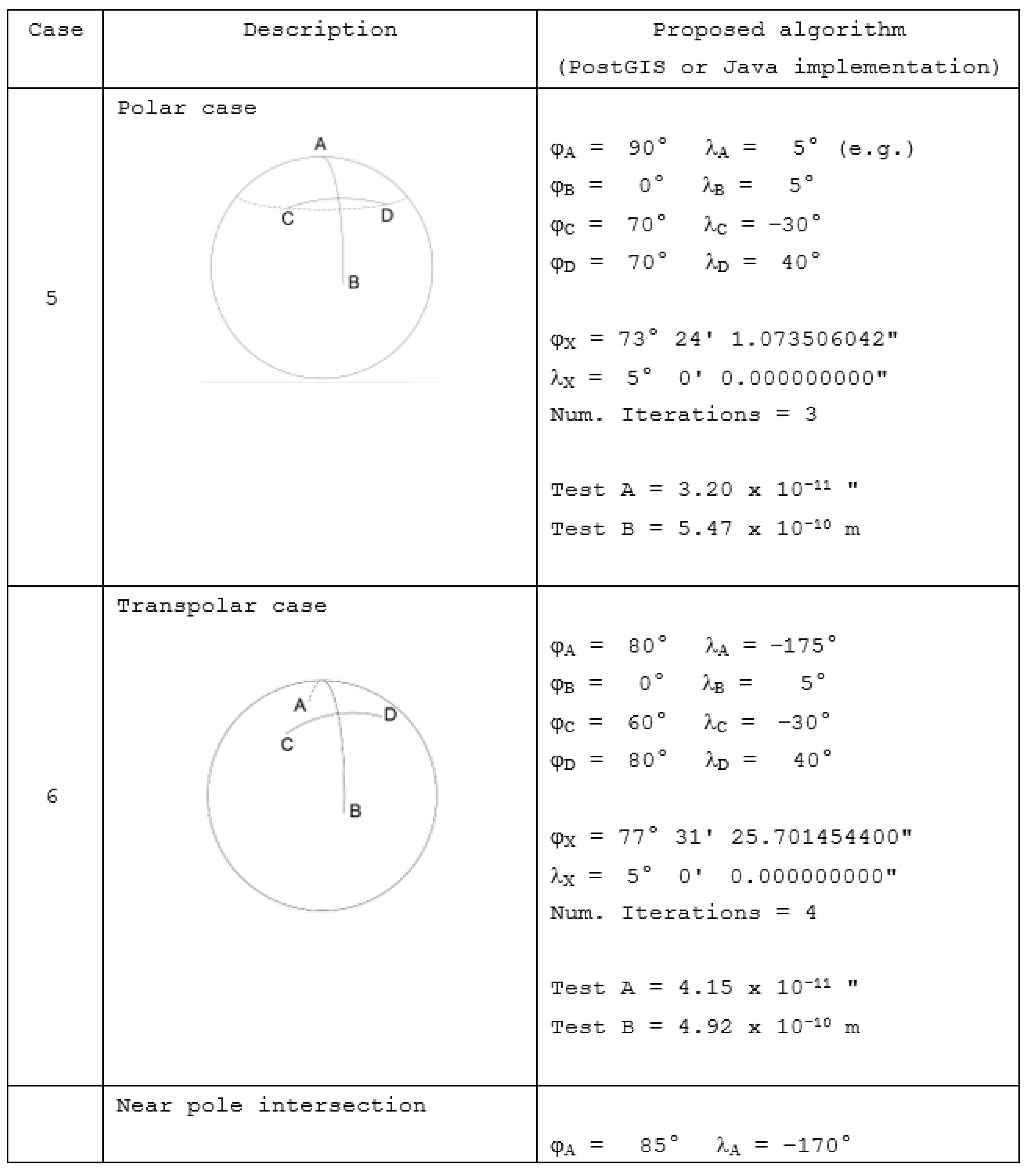
4.2. Special Geodesic Intersection Cases
The previous section proved that the proposed algorithm is working properly on the ellipsoid and giving a high accuracy, giving a true intersection on the ellipsoid.
Even so, to make sure a GIS user can use the algorithm in any case, more problematic geodesic intersections should be performed.
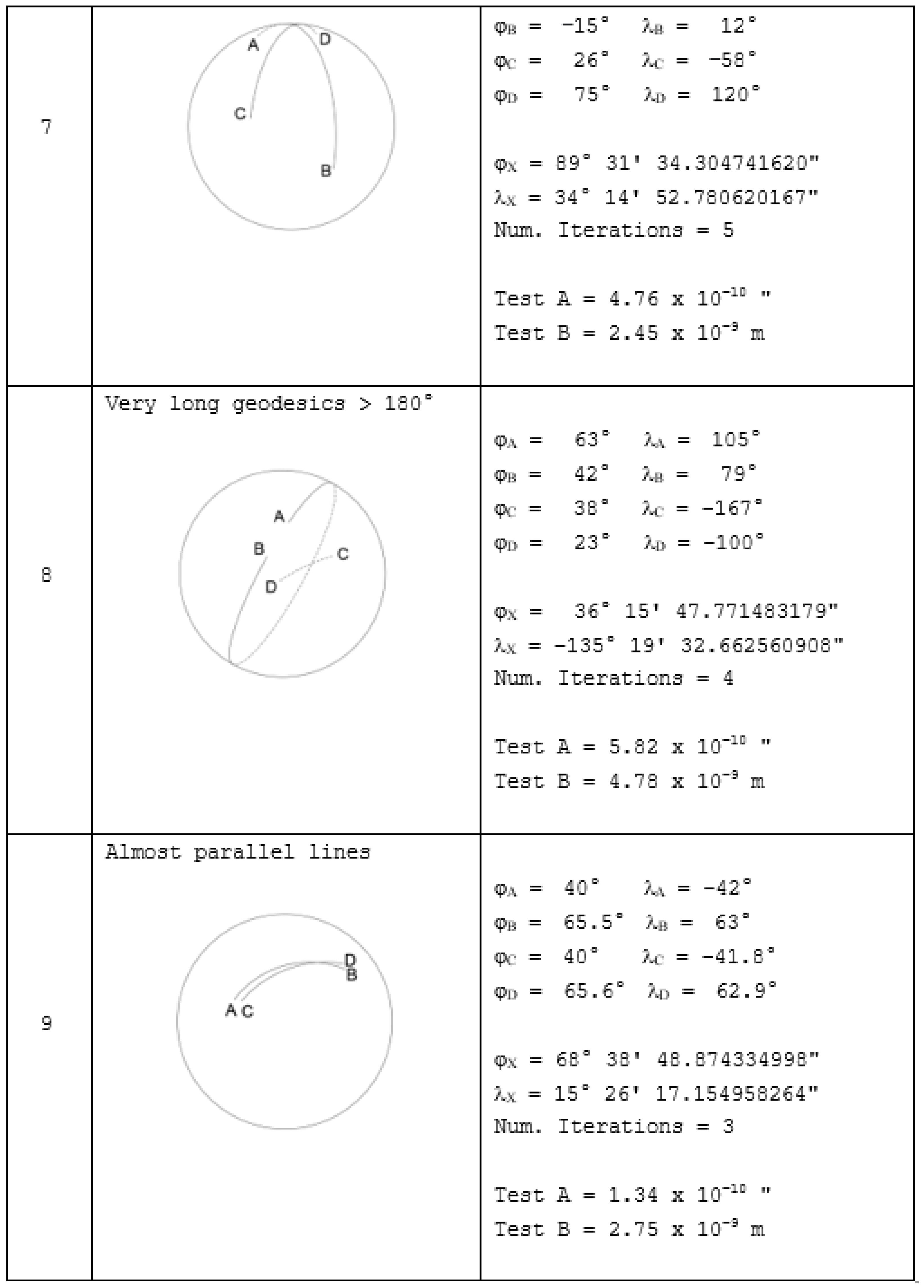
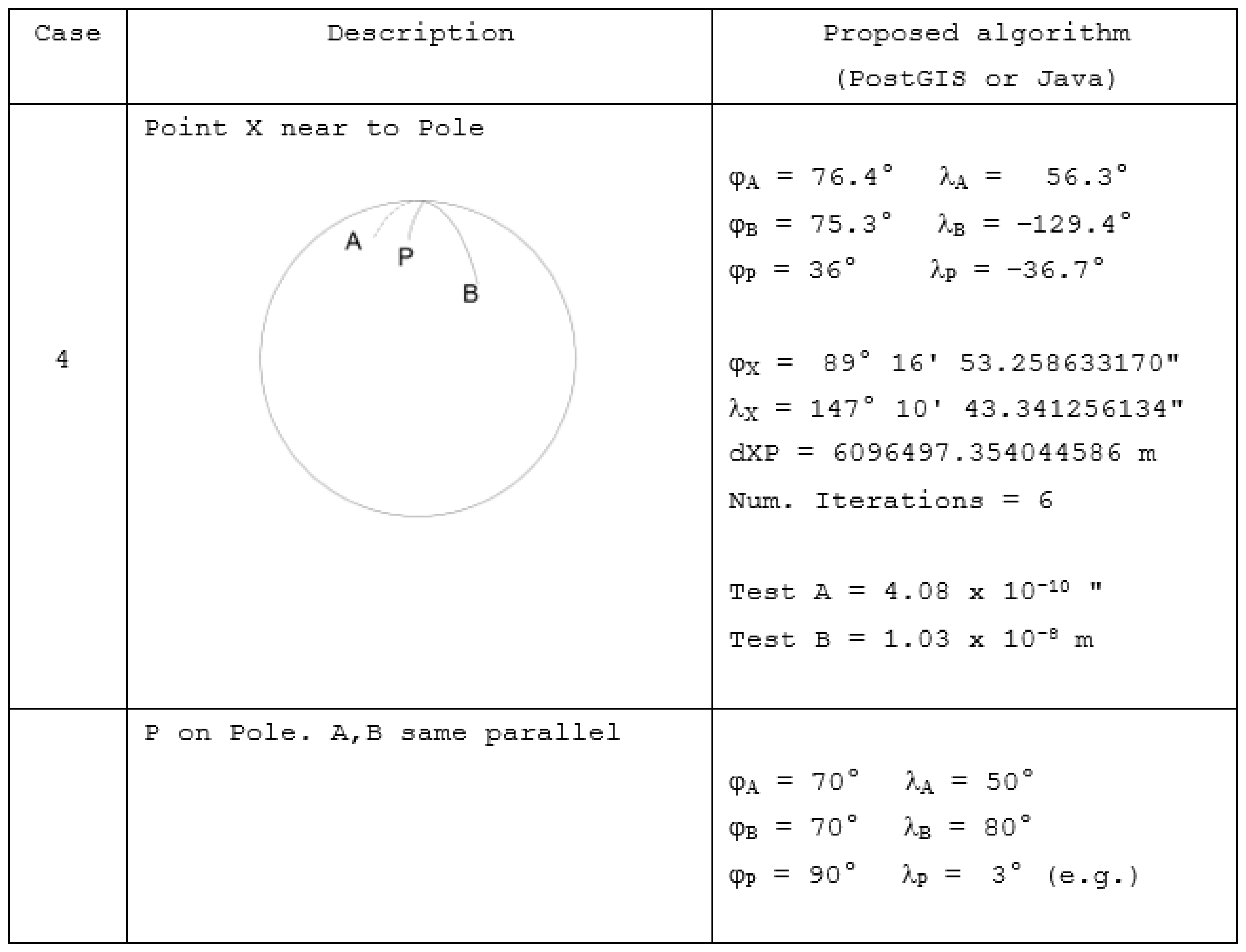
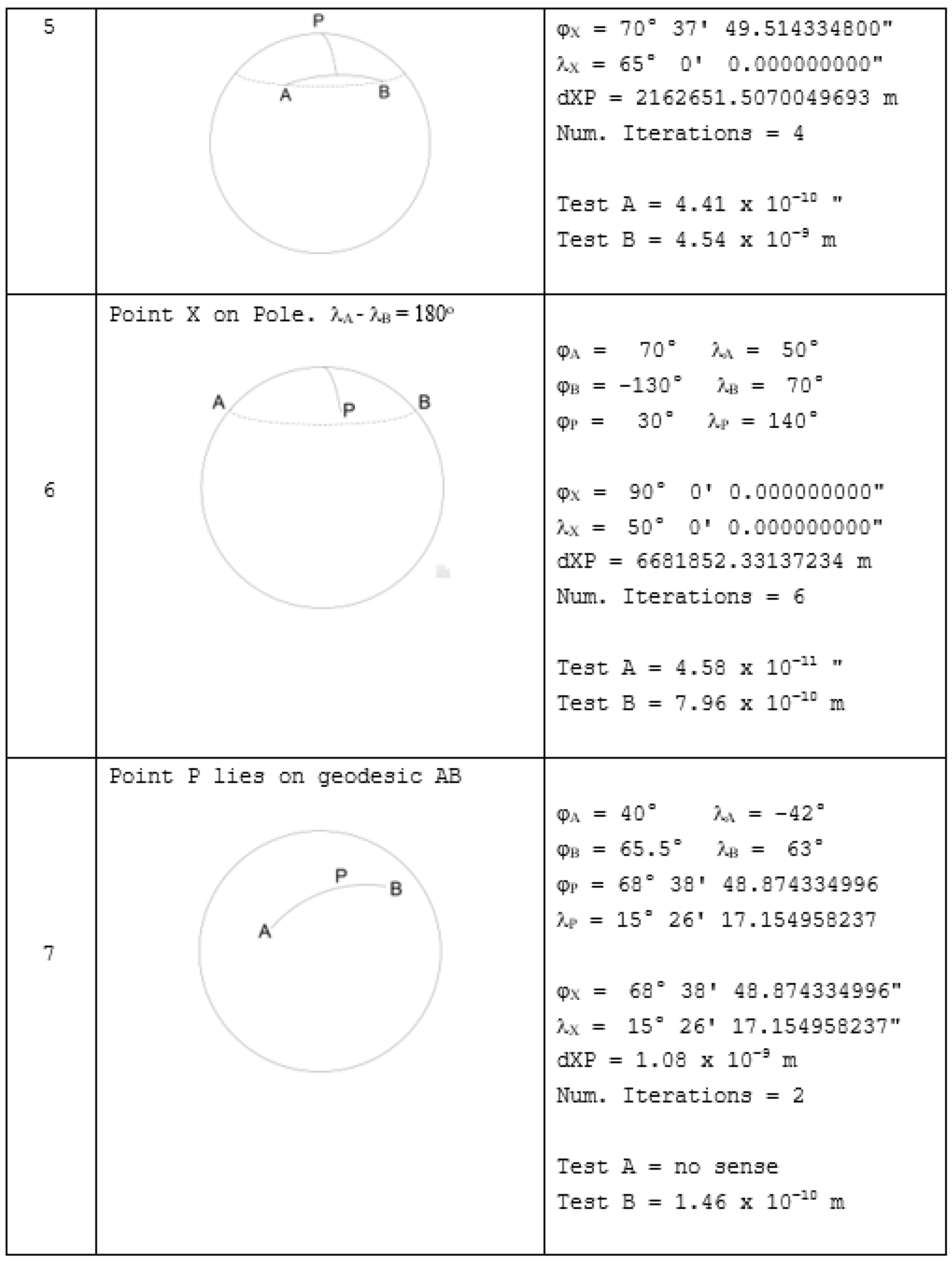
In this section, we add some new special cases that deal with polar, transpolar, very long (more than 180°) geodesics, etc. They are shown in
Scheme 8.
4.3. Minimum Distance from Point to Geodesic
Regarding the calculation of operation E (the minimum distance from a point P to a geodesic AB), the outcome is similar to the one obtained for operation D, i.e., all the software products discussed in
Section 2 provide approximate results.
The algorithm introduced by the authors in the previous article [
18] has a fast convergence to a nearly exact solution. However, we have just discovered its instability near the exact value due to a singularity in its Equation (10) which occurs at exactly the correct solution. Therefore, we decided to improve the algorithm for computing the minimum distance from a point P to a geodesic line AB as follows. Please note that steps (1) and (2) remain the same as in the previous work, the novelty is the introduction of step (3) now (the subsequent equation numbers and symbols refer to expressions in the previous article [
18]).
Compute the distance sAP and azimuths αAP and αAB by means of the implementation of the inverse problem of geodesy. Obtain angle A as the difference of these azimuths.
Obtain an approximate value for distances sPX and sAX by means of Equations (8) and (10) and compute the direct problem of geodesy from A with the distance sAX and azimuth αAX (which is the same as αAB) in order to obtain a point X which will act as point A in the next iteration.
For subsequent iterations, go back to steps (1) and (2) to obtain first sPX but replace the formula to obtain sAX by the following one, which has been obtained from the Napier pentagon for right-angle spherical triangles and unlike the one used in step (2) has no instabilities near the exact solution but a sharp convergence to it.
This formula has a singularity when sAP/R equals π/2 (i.e., sAP of some 10,000 km), which is the reason we preferred to obtain first an approximate sAP by means of Equation (10), preventing this singularity to happen in subsequent iterations (for which sAP has small values).
We implemented this algorithm in PostGIS and Java. The source code is publicly available in the repository [
25], files src/GeodesicSpatialOp.java and src/GeodesicSpatialOp.sql.
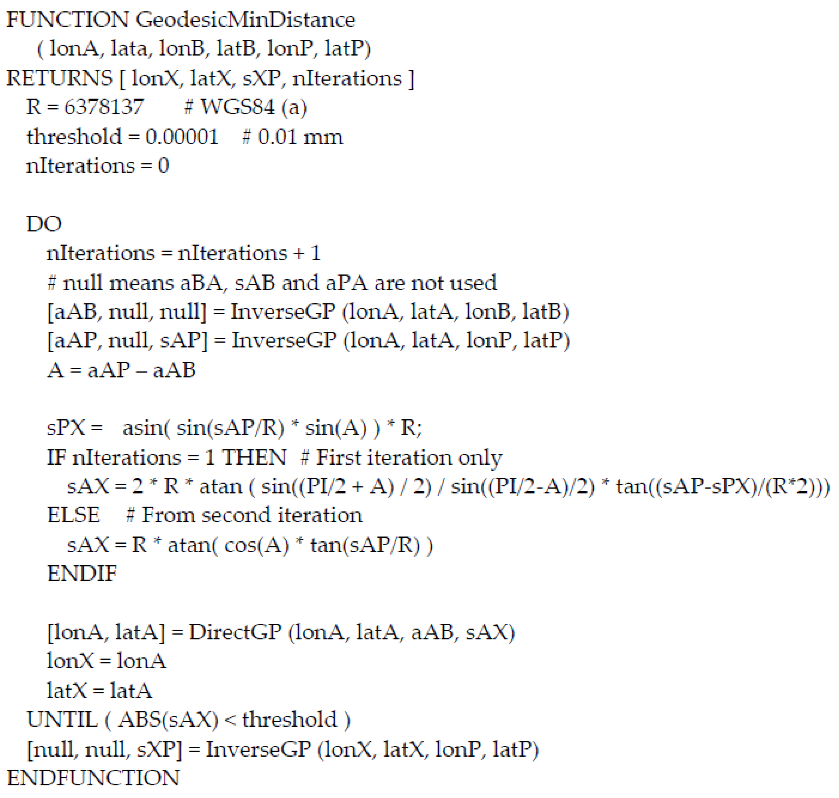
Scheme 9 shows the pseudocode of the Geodesic Minimum Distance algorithm, which returns the point X on the geodesic AB that is closest to the point P, and the minimum distance which is the length of the geodesic XP. The constraint is the azimuth XP that must be ±90°.
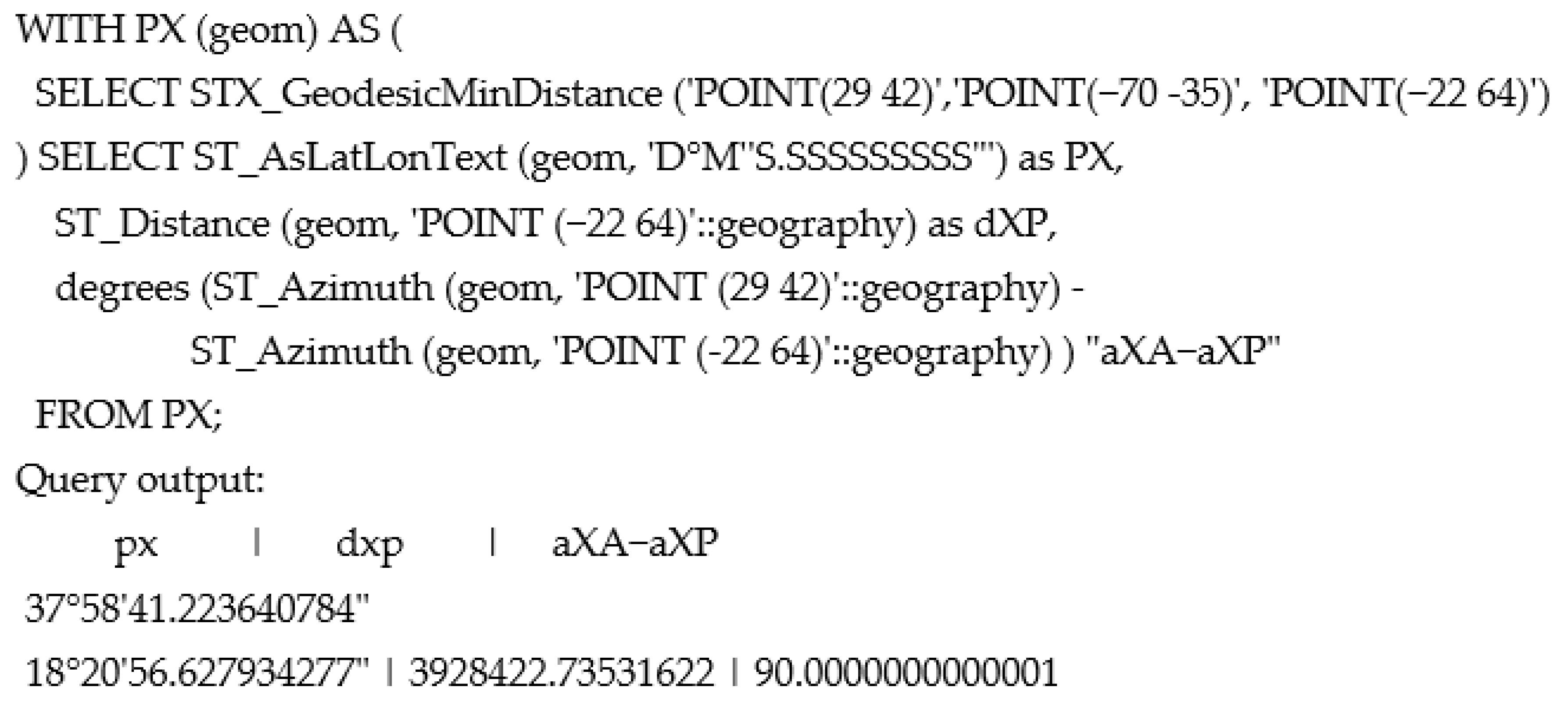
The new spatial PostGIS SQL function “STX_GeodesicMinDistance (a point, b point, p point)” calculates the minimum distance from the point P to the geodesic AB on the ellipsoid (WGS84 ellipsoid by default).
Scheme 10 shows how a SQL user can easily get the intersection of two geodesics. The example checks if the angle AXP is equal to 90 degrees.
To check the errors, we use slightly different tests A and B. The test A is similar to test A in the previous algorithm but considering now that the azimuth αXP must differ in 90 degrees with respect to the azimuths αXA and αXB, and, in addition, αAX = αAB. Test A formula is: Maximum (|αAX − αAB|, |αXP − αXA ± 90°|, |αXP − αXB ± 90°|).
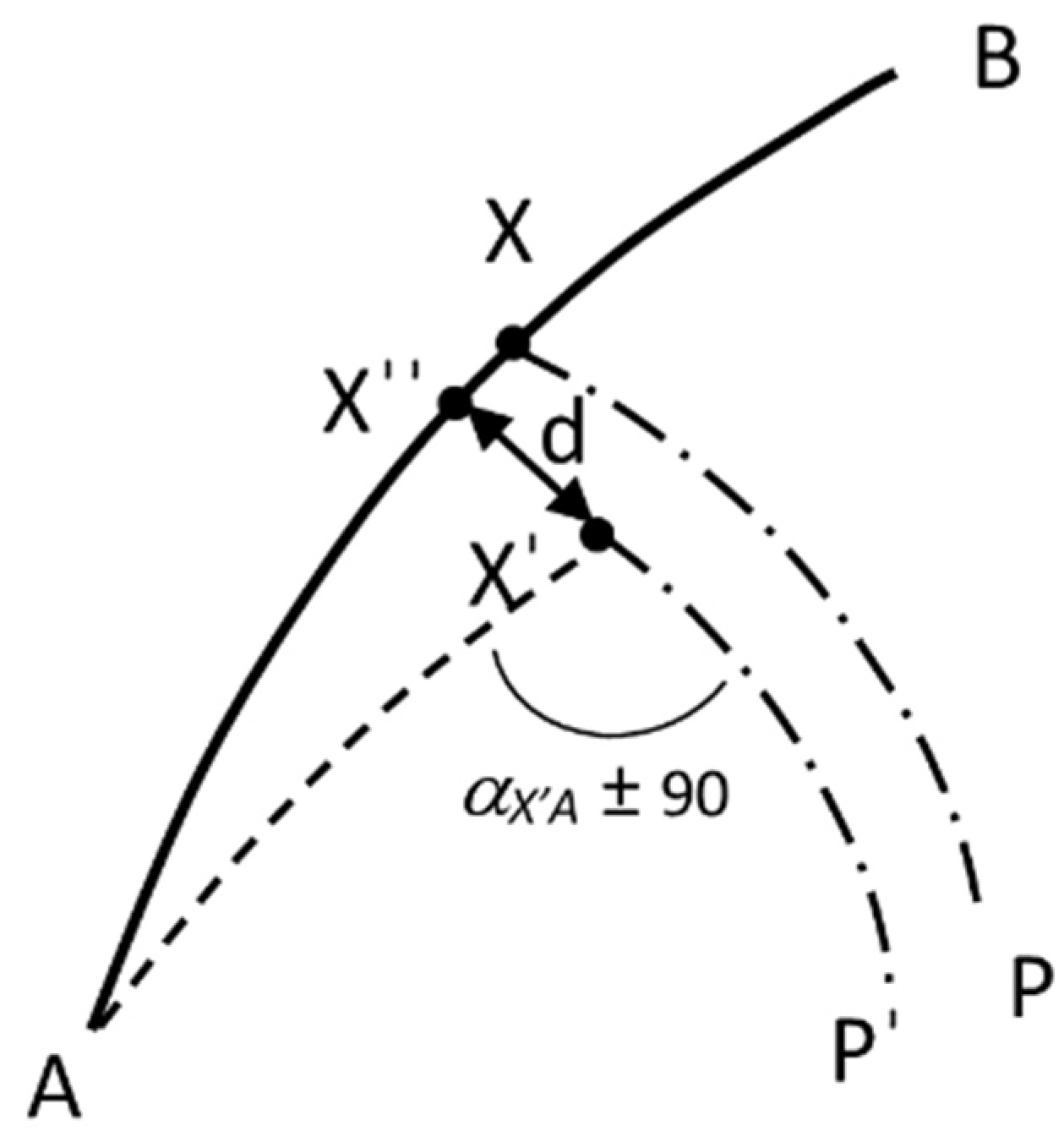
To perform test B, we calculate the deviation distance X′X″, plus a second deviation distance PP″. If an azimuth α
X′A ± 90° is applied from the point X′ plus a distance X′P (the distance X′X″ is close to zero), we will obtain a point P’’ that must coincide with the point P. If the distance PP″ is zero, it is guaranteed that the perpendicular to the geodesic through the point X crosses point P. Test B formula is: Maximum (X′X″, PP″),
Figure 4.
Table 5 shows the coordinates of the three examples used to test the algorithm whereas the column deviation of
Table 6 shows the result of both tests.
The largest difference of test B obtained for the 3 cases is 0.0041 μm. The computation coordinates of X are exact up to the ninth decimal place of arc seconds units, which represents a maximum of 0.03 μm. The minimum distance obtained can be correctly represented with up to the eighth decimal place (meters). We run these tests with Maxima, source code in tests/maxima_tests_minimumdistance.mac available at [
25].
Regarding to the running time, the operation E is approximately twice as fast as operation D, obtaining 40,000 times per second in cases 2 and 3 (four iterations to converge) and 60,000 times per second in case 1 (three iterations).
Table 7 shows the minimum distance differences obtained between the software products and the results from
Table 6.
We can see that ArcGIS is the only studied software with deviations of 1 cm or less, although the distance PP″ (test B) happens to lie up to several meters off (0.05 m for Case 1, 2.5 m for Case 2 and 4.2 m for Case 3), which means the point X on the geodesic is indeed not well calculated.
Unlike operation D, Oracle and Google implement different algorithms. The deviations in cases 2 and 3 reach up to 5000 m.
Scheme 11 shows some additional special cases: polar, transpolar, 180° long geodesics, etc.
5. Conclusions
We demonstrated that some of the most powerful spatial analysis software solutions perform some geodetic calculations approximately. Two of these operations are the intersection of two geodesics and the minimum distance from a point to a geodesic.
These operations are critical to implement a true geodetic spatial analysis engine, since many other more complex spatial processes are based on them, therefore, they must be calculated with high accuracy, that is close to machine precision (so that, in practice, they are insignificantly affected by numerical truncations).
The deviations committed by these popular spatial analysis software are large, easily exceeding the necessary tolerances according to the spatial analysis objectives. Even for geodesics of a few kilometers the best studied solution gave us deviations of centimeters. For longer lines they showed deviations of meters.
We presented two algorithms in Java and PostGIS that perform high accuracy calculations on the ellipsoid using double precision types, achieving an error lower than 100 nm in both operations. The implementation of this algorithm provides the following features:
The accuracy obtained is higher than using local projections even considering very short distances.
It allows a highly accurate spatial analysis even in large extensions of territory (national, continental or global).
Worrying about choosing the best-fit projection for analyzing the data becomes unnecessary, since we do not need to use any projection.
A good performance (considering the spatial analysis is on the ellipsoid) is achieved (20,000 geodesic intersections per second) due to a fast convergence process. The worst scenario took six iterations, if the final accuracy goal is µm instead of nm we can reduce the number of iterations by one or two. The proposed algorithm is fast enough to allow the migration of flat computational geometry libraries (JTS, GDAL, etc.) to computational geometries libraries on the ellipsoid. This way, a full spatial analysis software solution on the ellipsoid could be offered for the first time.
Consequently, we propose the following final recommendations for practical use when preparing a geodetic spatial analysis engine:
Some of the most renowned spatial analysis software solutions rely on the use of auxiliary map projections to solve problems on the surface of the ellipsoid which may produce manifestly incorrect results. These auxiliary map projections must be abandoned altogether in favor of reliable algorithms for direct computation on the ellipsoid surface that produce accurate results irrespectively of the extension of the area of interest.
In recent times: algorithms that yield results of an accuracy close to machine precision have been developed. This is the case of Karney’s implementation of the direct and inverse problems of geodesy [
14] and Transverse Mercator formulas with an accuracy of a few nanometers [
36], which are included in GeographicLib [
13]. This is also the case of the algorithms for intersection of geodesics and minimum point-to-geodesic distance presented in this paper. Spatial analysis software solutions should incorporate these solutions in order to provide the user with the highest possible accuracy, that is, an accuracy close to machine precision.
When performing geometric calculations on the ellipsoid surface, such as determination of the intersection of geodesics or minimum point-to-geodesic distance, suitable tests for validating the solution (such as the ones used in this paper) should be applied to ensure the degree of accuracy of the solution obtained.


