Distributed 3-D Path Planning for Multi-UAVs with Full Area Surveillance Based on Particle Swarm Optimization

Abstract

Collision-free distributed path planning for the swarm of unmanned aerial vehicles (UAVs) in a stochastic and dynamic environment is an emerging and challenging subject for research in the field of a communication system. Monitoring the methods and approaches for multi-UAVs with full area surveillance is needed in both military and civilian applications, in order to protect human beings and infrastructure, as well as their social security. To perform the path planning for multiple unmanned aerial vehicles, we propose a trajectory planner based on Particle Swarm Optimization (PSO) algorithm to derive a distributed full coverage optimal path planning, and a trajectory planner is developed using a dynamic fitness function. In this paper, to obtain dynamic fitness, we implemented the PSO algorithm independently in each UAV, by maximizing the fitness function and minimizing the cost function. Simulation results show that the proposed distributed path planning algorithm generates feasible optimal trajectories and update maps for the swarm of UAVs to surveil the entire area of interest.

1. Introduction

Unmanned Aerial Vehicles (UAVs), known as drones, gained much popularity in the area of surveillance due to their capability in vertical take-off and landing, and high maneuverability, which provides various benefits in various platforms or environments. UAVs can be also used for surveilling [1] providing security to the larger government or private area known as estates [2], and also can be used for sensing and data collection [3,4]. However, when defining a mission, path planning plays a basic and crucial role in the whole system. Generally speaking, when designing a path for UAV, it should reflect various factors, including dynamic target point, obstacles avoidance both statically and dynamically, the shortest pathfinding, as well as mission planning while surveilling. Nowadays, UAVs are widely used for various purposes, especially for surveilling because of the small size and lightweight, easy operational procedure, and tremendous benefits of easy access from one place to another place. UAVs are gaining more popularity in surveillance. For this reason, path planning for UAVs is more crucial, and it plays a fundamental role in the autonomous flight system for unmanned aerial vehicles (UAVs). It refers to the optimal path planning problem of an unmanned aircraft, which can be formulated as an optimization problem of finding the most compatible path from source to destination. The feasible trajectory is usually correlated with the path minimizing certain optimization indexes, for example, energy consumption, flight risk, path length, etc. of certain path planning missions.

1.1. Related Work

While thinking about generating path planning for UAVs, we have to consider the scenario, whether it is a two-dimensional (2-D) environment or a three-dimensional (3-D) environment. There are various path planning strategies regarding both 2-D and 3-D environments. As we are working with UAVs, which are related to the 3-D environment, we have focused mainly on path planning in the 3-D environment. There are so many path planning algorithms regarding the 3-D environment, which can be categorized into five categories [5]. These include, (i) Sampling-Based Algorithms, like, visibility graph, corridor map [6], Rapidly-exploring Random Tree (RRT) [7], 3-D Voronoi [8] (ii) Node Based Optimal Algorithms, such as, Dijkstra’s Algorithm [9], A* algorithm [10], D* algorithm [11], (iii) Mathematics Model-Based Algorithms, like, Linear Programming and Optimal Control [12], Binary Linear Programming [13], Nonlinear Programming [14,15], (iv) Bio-inspired Algorithms, which can be divided into two types, Evolutionary Algorithm [16], and Neural Network [17], and (v) Multi-fusion Based Algorithms [18]. There are various types of Evolutionary Algorithm, such as, Genetic Algorithm [19], Memetic Algorithm [20], Particle Swarm Optimization (PSO) [21], and Ant Colony Optimization (ACO) [22], which are notable for the path planning of UAVs in the 3-D environment. Evolutionary Algorithms are the algorithms that update the results in iteration-by-iterations. In our proposed 3-D path planning methodology, we used Particle Swarm Optimization (PSO), due to its benefits like the advantages of easy implementation, simple parameter settings, fast convergence speed, and for which the PSO algorithm has been widely used in various fields, such as, functions optimization, neural networks training, and fuzzy logic system control are notable. However, it has some limitations too, like premature convergence, route self-crossing. The authors in [23] suggest that this problem can be solved by using the following techniques, (1) adjust important parameters iteratively; (2) random grouping inversion strategy for avoiding premature convergence. In terms of area coverage, various techniques have been suggested by various authors, such as the authors in [24] decomposed the concave region into a convex sub-region, then the flight direction was determined based on the width of the convex polygon. Some adjacent sub-areas were merged to avoid unnecessary repetitive movement. In [25], the authors proposed a new approach relative to UAVs’ capabilities assessment by using hierarchical fuzzy inference and established a cost model for UAVs’ mission execution. The authors in [26], believed that a rectangle can be circumscribed by any polygon. The idea of polygon region segmentation was adopted by the authors in [27]. The sweeping technique was used for area decomposition by the authors in [28], to minimize the number of UAV, turns inside the subareas by generating the optimal number of lanes. In [29], for moving targets, the formation coverage search method was proposed. The authors in [30,31,32,33] discussed distributed path planning using the PSO algorithm and the designing of the quadrotor control.

1.2. Main Contributions

The objective of this paper is to develop a distributed path planner for multi-UAVs with full coverage for certain operational areas with a priority-based mechanism. For this, we propose a distributed trajectory planner based on Particle Swarm Optimization (PSO) and Bresenham Algorithm. PSO is used to generate the optimal trajectory, while the Bresenham algorithm is used for ensuring the full coverage of the operational area. To generate the optimal trajectory, we propose a multi-objective fitness function, where energy consumption and flight risk are taken care of, as well as the maneuverability and feasibility of the paths are taken into consideration.

This paper is organized as follows, we provide a System Model for UAVs Path Planning and representation of the operational area in Section 2. In Section 3, we discuss the mathematical model for optimal trajectory planning. In this section, we design the Dynamic Fitness Function of the Objective and Constraint function of UAVs. In Section 4, we propose a distributed trajectory planner based on PSO and Bresenham algorithm. Section 5 contains Simulation results and discussions about our implementation of the proposed trajectory planner. In Section 6, we conclude our paper.

2. System Model for UAV Path Planning

We have built a Matlab-based operational environment where we mimicked a real-life environment like terrain and flat surfaces to represent the 3-D environment. This work is a continuation of our previous work [1], where we derived the optimal surveillance trajectory for multiple UAVs and detected the existence of any illegal UAVs, which had a centralized control system. In that scenario, the trajectory planner did not have the functionality of full coverage for a certain operational area. In this paper, we developed a system model for full coverage of the operational area for multi-UAVs in a distributed manner along with a priority-based mechanism.

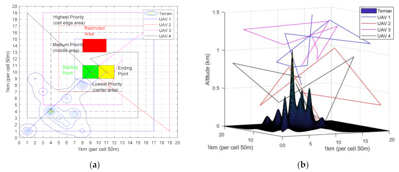
2.1. Problem Description

In our operational scenario, which is a 3D operational space with local maxima was surveilled by the monitoring drones with specifications mentioned by Hu Teng et al. [1], which were employed to detect the existence of illegal drones. During the surveillance, we explain that the monitoring drone cannot infiltrate any sensitive or important area, which is restricted by regulations. To avoid complexity or being destroyed as a hostile drone, we stipulate that the monitoring drone cannot also access the ground-base station (GBs) area, which is equipped with ground-based drone detection systems. Furthermore, the communication between monitoring drones is done with each other in an ad-hoc manner or UAV-to-ground link communication system. Therefore, monitoring drones can share information mutually during the execution of flight assignments. In our implementation, we set our operational area into a 20 × 20 grid matrix and differentiated the whole operational space into several small unit areas, known as cells, where some cells are considered as restricted areas. Operational area representation and proposed trajectory planning are discussed in the following sections.

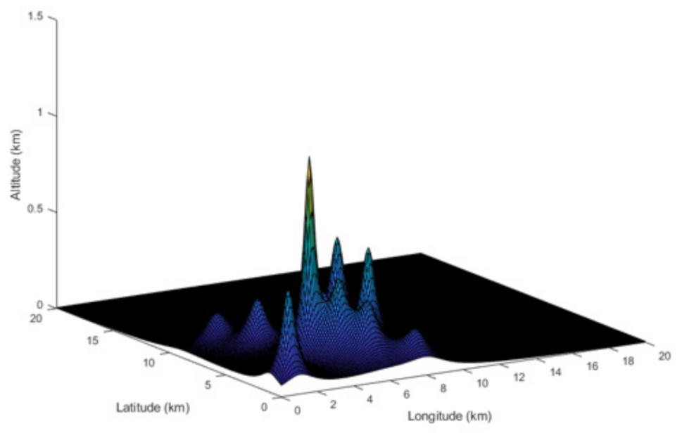
2.2. Operational Area Representation

To resemble a real-life environment, we adopt a variation of the Foxhole Shekel function in our paper to represent the terrain, shown in Figure 1, which is formulated as expressed in Equation (1) [34],

$$F_k\left(x\right)\hspace{0.17em}=\hspace{0.17em}{{\displaystyle \sum }}_{a\hspace{0.17em}=\hspace{0.17em}1}^{10}\frac{0.1}{{{\displaystyle \sum }}_{b=1}^{10}{\left(x_b-{\eta }_{ab}\right)}^2+{\gamma }_a}$$

(1)

where parameters η and $\gamma$ are used to vary the shape of the terrain. We adopted this terrain because there is a shortage of widely-accepted benchmarks in the field of trajectory planning for UAVs. Therefore, the local maxima of the landscape can be considered mountains [34].

2.3. Trajectory Planning

In our proposed path planning, we generated a trajectory in a sequence of waypoints in three-dimensional space using the particle swarm optimization algorithm [1]. Therefore, vector form is used for encoding feasible path where the vector element $T_i$ = ($a_i,\hspace{0.17em}bi,\hspace{0.17em}{c}_i$) can be used for representing the ith waypoint, which can be shown as,

$$T_r\hspace{0.17em}=\hspace{0.17em}{T}_1,T_2,T_3,\dots ,T_{N_w}$$

(2)

where $N_w$ is known as the number of waypoints in a feasible trajectory, $r$ and $w$ are positive integer numbers, and the number of trajectories is proportional to the number of waypoints.

3. Mathematical Model for Optimal Trajectory Planning

A technique in this paper is introduced based on a distributed path planning, where each UAV is equipped with a PSO optimization algorithm. The trajectories are, thus, not computed in a central unit, but in a distributed manner on the swarm of UAV. Therefore, the communication between the swarm of UAV is only used to share position and location among themselves, which is considered as a target to be tracked; each UAV then computes its trajectory. Therefore, this results in a distributed path planning. To design a mathematical model for an optimal trajectory planner we designed the required functions to get dynamic fitness values. The design of function consists of three types, such as fitness function, objective function, and constraint function. The mathematical model for these optimal functions is discussed in the following sections.

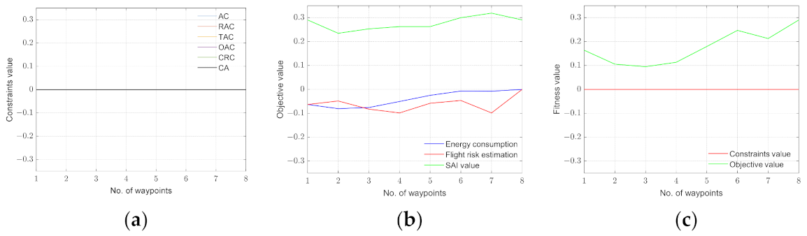
3.1. Dynamic Fitness Function Design

In this section, we propose a multi-objective fitness function consisting of eight optimization indexes to assess the trajectories generated by the proposed multi-UAVs path planning algorithm. We divided optimization indexes into two groups and assign different priority levels. This is due to the different importance of optimization indexes during the optimization process. They are known as, (1) the optimization objectives, which need to maximize their value to derive an optimal trajectory, and (2) the constraints which must satisfy by UAVs due to their physical limitations.

Table 1. Optimization index Classification.

Objective Function
Name	Energy Consumption		Flight Risk Estimation		Surveillance Area Importance
Abbreviation	EC		FRE		SAI
Equation	(5)–(10)		(11)–(14)		(15)–(17)
Value/Range	[0, 1]		[0, 1]		[0, 1]
Constraint Function
Name	Aerial Constraint	Restricted Area Constraint	Turning Angle Constraint	Operational Area Constraint	Coverage Range Constraint	Collision Avoidance
Abbreviation	AC	RAC	TAC	OAC	CRC	CA
Equation	(19)	(20)	(21)	(22)	(23)	(24)
Value/Range	0	0	0	0	0	0

shows these classifications and the equations to calculate them. Therefore, we formulate the dynamic fitness function as,

$$F_{dynamic\_fitness}\hspace{0.17em}=\hspace{0.17em}{F}_{obj}\hspace{0.17em}+\hspace{0.17em}{F}_{const}$$

(3)

where $F_{obj}$ is the objective function, focusing to gain maximum values in terms of other parameters, $F_{const}$ is the physical and environmental limitations, should be accomplished before trajectory planning.

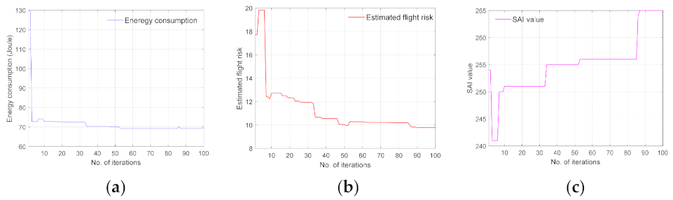
3.2. Objective Function Design

We defined the objective function as an optimization criterion to improve the quality of path planning [1]. Therefore, we define the objective function as a weighted component of energy consumption, flight risk estimation, and important area surveillance and formulated the objective function as in Equation (4),

$$F_{obj}=\hspace{0.17em}-w_1{F}_{EC}-w_2{F}_{FRE}+w_3{F}_{SAI}$$

(4)

where F_EC, F_FRE, and F_SAI are defined to be in the range of [0, 1] and w_i (i = 1, 2, 3) were used for expressing the weight of the objective component. Our main focus was on generating the optimum path with less energy consumption, environmental flight risk, but higher surveillance. Therefore, we designate surveillance area importance as the positive and the rest areas negative values.

3.2.1. Energy Consumption (EC)

Due to the physical limitations of small UAV, like battery power management, we need to design the path for UAV carefully so that it can surveille the path within its limited battery power. Therefore, it is always preferable to a path with less fuel consumption. Assuming the UAV having constant velocity during the operation time, then we formulated energy consumption, EC as,

$$F_{EC}=\frac{{{\displaystyle \sum }}_{i=1}^{N_w-1}E{C}_i}{maxEC}$$

(5)

where,

$$E{C}_i=P_w\ast t_{i,i+1}$$

(6)

$$t_{i,i+1}=\frac{d_{i,i+1}}{v}$$

(7)

$$d_{i,i+1}=\sqrt{{\left(x_{i+1}-x_i\right)}^2+{\left(y_{i+1}-y_i\right)}^2+{\left(z_{i+1}-z_i\right)}^2}$$

(8)

where EC_i is the energy consumption from the ith waypoint to (i + 1)th waypoint. P_w the energy consumption of the UAV at velocity $v$ for unit time, while t_i,i+1 is the duration of flight time taken by UAV from ith waypoint to (i + 1)th waypoint. d_i,i+1 is the Cartesian distance of a flight from ith waypoint to (i + 1)th waypoint. We normalized the energy consumption and formulated it as, max EC,

$$maxEC=\left(N_w-1\right)\ast P_w\ast \frac{d_{max}}{v}$$

(9)

where,

$$d_{max}=\sqrt{X^2+Y^2+Z^2}$$

(10)

where X, Y, and Z are the boundary condition of operation space in the 3-D environment.

3.2.2. Flight Risk Estimation (FRE)

Some physical limitations need to be overcome during flight time as those limitations make the UAV vulnerable to harsh weather conditions during the surveillance, like rain, strong winds or snow, etc. Additionally, flying at high altitudes can be another big risk as higher altitudes pose stronger winds, which may increase the risk or uncertainty of being accidentally destroyed. Based on the above scenario, we define two kinds of flight risks:

• Environmental Risk

The environment consists of a wide range of random characteristics variables which makes it difficult to build a model that precisely measures the environmental risk. Therefore, for removing complexity, we randomly generated an environmental risk value for each waypoint. That is, environmental risk, $r_{i,\hspace{0.17em}i\hspace{0.17em}+\hspace{0.17em}1}^{er}$, between the ith waypoint and (i + 1)th waypoint is defined as the sum of their environmental values.

• High Altitude Risk

High altitude risk is an absolute difference in flying altitude between the two waypoints. High altitude risk, $r_{i,\hspace{0.17em}i\hspace{0.17em}+\hspace{0.17em}1}^{har}$, can be formulated as,

$$r_{i,\hspace{0.17em}i\hspace{0.17em}+\hspace{0.17em}1}^{har}=\hspace{0.17em}\eta \ast \left(z_{i+1}-z_i\right)$$

(11)

where $\eta$ represents a constant parameter control.

Since the flying risk a location-dependent parameter, it changes accordingly to the environment depending only on the weather conditions and flying altitude during the flight time. Therefore, flight risk estimation can be formulated as from Equations (12)–(14),

$$F_{FRE}=\frac{{{\displaystyle \sum }}_{i\hspace{0.17em}=\hspace{0.17em}1}^{N_w-1}FR{E}_i}{maxFRE}$$

(12)

$$FR{E}_i={\phi }_{ER}{r}_{i,i+1}^{er}+{\phi }_{HAR}{r}_{i,i+1}^{har}$$

(13)

where FRE_i is the flight risk estimation from the ith waypoint to the (i + 1)th waypoint, ${\phi }_{HAR}$ is the total high altitude risk, and ${\phi }_{ER}$ is total environmental risk. We normalized the flight risk estimation and formulated it as, max FRE:

$$maxFRE=\left(N_w-1\right)\ast \left[{\phi }_{HAR}\ast Z+{\phi }_{ER}\ast \left(2\ast max{r}^{er}\right)\right]$$

(14)

where maxr^er represents the maximal environmental risk.

3.2.3. Surveillance Area Important (SAI)

We divided the whole operational area into three different important levels, which are considered the cell edge area, middle area, and center area of the total operational area. Cell edge areas are the areas that are located in the boundary line of operational areas, and the middle areas are the adjacent cells or inner cells of our operational area. Since the penetration of any illegal drones directly come from the edge area, we have assigned the highest priority of surveillance to those areas, which means the cell edge area should be surveilled first in our implementation. Whereas the center cells are the most secured area among the total operational area, we assigned the least SAI Value for the center area. In this way, we have assigned the order of priority to surveille whole area coverage. The normalized SAI value can be calculated by Equations (15)–(17),

$$F_{SAI}=\frac{{{\displaystyle \sum }}_{i=1}^{N_w}SA{I}_i\left(t\right)}{maxSAI}$$

(15)

$$SA{I}_i={{\displaystyle \sum }}_{cell\hspace{0.17em}xϵN\left(i\right)}{v}_{cellx}\left(t\right)$$

(16)

$$maxSAI=N_w\ast N_i\ast v_{max}$$

(17)

where $SA{I}_i\left(t\right)$ the SAI values of the ith waypoint, $v_{cellx}\left(t\right)$ is the cell value of x at the tth flight time, $N_i\hspace{0.17em}$ is the supervised cell set from the ith waypoint, $v_{max}$ is the maximal SAI value.

3.3. Constraint Function Design

A negative constraint function was designed to evaluate the feasibility of generated path. This is due to the regulations of the external environment, which the UAV has to follow like UAV cannot through a military base, sensitive govt. area etc. When they fulfill the conditions, each constraint is set to be equal to 0, otherwise, a negative penalty value P is given. A brief description of the constraint function is given below. We formulated the constraint function as:

$$F_{const}=AC+RAC+TAC+OAC+CRC+CA.\hspace{0.17em}$$

(18)

3.3.1. Aerial Constraint (AC)

While generating a feasible path, monitoring drones should consider terrain areas as monitoring drones cannot go through the terrain area to avoid collisions with mountains. To avoid collisions, the flying altitude of monitoring drones should be higher than the terrain altitude. We represented terrain in aerial constraint which can be described as:

$$AC=0,\hspace{0.17em}AC={{\displaystyle \sum }}_{i=1}^{N_w}A{C}_i$$

(19)

where,

$$A{C}_i=\left\{\begin{array}{c}P,\hspace{0.17em}\hspace{0.17em}\hspace{0.17em}\hspace{0.17em}\hspace{0.17em}\hspace{0.17em}if\hspace{0.17em}{z}_j<Area\left(x_i,y_i\right)\\ \hspace{0.17em}\hspace{0.17em}\hspace{0.17em}0,\hspace{0.17em}\hspace{0.17em}\hspace{0.17em}\hspace{0.17em}\hspace{0.17em}\hspace{0.17em}otherwise\hspace{0.17em}\hspace{0.17em}\hspace{0.17em}\hspace{0.17em}\hspace{0.17em}\hspace{0.17em}\hspace{0.17em}\hspace{0.17em}\end{array}\right.$$

3.3.2. Restricted Area Constraint (RAC)

For some specific areas (e.g., government-sensitive regions), monitoring drones cannot be allowed to enter due to the regulations. A legal path should be carefully designed to avoid those forbidden areas. For simplicity, we assume that those forbidden areas are rectangles. Therefore, the forbidden area constraint can be formulated as:

$$RAC=0,\hspace{0.17em}RAC={{\displaystyle \sum }}_{i=1}^{N_w}RA{C}_i$$

(20)

where,

$$RA{C}_i=\left\{\begin{array}{c}P,\hspace{0.17em}if\hspace{0.17em}waypoint\hspace{0.17em}in\hspace{0.17em}range\left(x_j,y_j\right)\\ 0,\hspace{0.17em}otherwise\hspace{0.17em}\hspace{0.17em}\hspace{0.17em}\hspace{0.17em}\hspace{0.17em}\hspace{0.17em}\hspace{0.17em}\hspace{0.17em}\hspace{0.17em}\hspace{0.17em}\hspace{0.17em}\hspace{0.17em}\hspace{0.17em}\hspace{0.17em}\hspace{0.17em}\hspace{0.17em}\hspace{0.17em}\hspace{0.17em}\end{array}\right.$$

where,

$$range(x_j,y_j)\hspace{0.17em}=\hspace{0.17em}\{l_x\le x_j\le u_x\}\hspace{0.17em}\cap \hspace{0.17em}\{l_y\le y_j\le u_y\}\hspace{0.17em}$$

where $N_w$ is the number of waypoints, $l_x,l_y$ are the lower bounds of x and y, $u_x$, $u_y$ is the upper bounds of x and y.

3.3.3. Turning Angle Constraint (TAC)

The turning angle explains the maneuverability of a UAV during the flight from the previous and current directions [1,35,36]. The Path for UAVs should be adequately smooth to maneuver through easily [37]. Therefore, the turning angle of the UAV is required to be less than the maximum turning angle [35]. This constraint can be formulated as follows,

$$TAC=0,TAC={\displaystyle \sum }_{i=2}^{N_w-1}TA{C}_i$$

(21)

where,

$$TA{C}_i=\left\{\begin{array}{c}P,\hspace{0.17em}if\theta >{\theta }_{max}\\ 0,\hspace{0.17em}otherwise\hspace{0.17em}\end{array}\right.$$

where $\theta$ defines the turning angle of the UAV in 3-D directions ($x_i,\hspace{0.17em}{y}_i,\hspace{0.17em}{z}_i$), and ${\theta }_{max}$ is the maximum tolerable turning angle.

3.3.4. Operational Area Constraint (OAC)

For feasible path planning, the UAV must stay inside the operational area to avoid ambiguity. Thus, a negative penalty P is added in the constraint function if any unwanted event occurs. The operational area constraint of a mission can be formulated as follows:

$$OAC=0,\hspace{0.17em}OAC={{\displaystyle \sum }}_{i=1}^{N_w}OA{C}_i$$

(22)

where,

$$\hspace{0.17em}OA{C}_i=\left\{\begin{array}{c}0,\hspace{0.17em}if\hspace{0.17em}waypoint\hspace{0.17em}in\hspace{0.17em}map\left(x_j,y_j\right)\hspace{0.17em}\hspace{0.17em}\\ P,\hspace{0.17em}otherwise\hspace{0.17em}\hspace{0.17em}\hspace{0.17em}\hspace{0.17em}\hspace{0.17em}\hspace{0.17em}\hspace{0.17em}\hspace{0.17em}\hspace{0.17em}\hspace{0.17em}\hspace{0.17em}\hspace{0.17em}\hspace{0.17em}\hspace{0.17em}\hspace{0.17em}\hspace{0.17em}\hspace{0.17em}\hspace{0.17em}\end{array}\right.$$

where,

$$range(x_j,y_j)\hspace{0.17em}=\hspace{0.17em}\{l_x\le x_j\le u_x\}\hspace{0.17em}\cap \hspace{0.17em}\{l_y\le y_j\le u_y\}\hspace{0.17em}$$

where $N_w$ is the number of waypoints, $l_x,l_y$ are the lower bounds of x and y, $u_x$, $u_y$ is the upper bounds of x, and y, respectively.

3.3.5. Coverage Range Constraints (CRC)

For the whole coverage, UAV needs to surveille all the areas. If the path planning includes the coverage area, no penalty is given. Otherwise, a negative value is given as a penalty. When the trajectory is generated for each particle, its waypoint values are compared with the important area’s waypoint value. The important area’s waypoints value are divided into 4 sub-areas. If any value falls between those ranges, no penalty is given. Otherwise, a negative penalty is given. Then, that waypoint’s value is updated accordingly. Coverage range constraint can be formulated as:

$$CRC=\hspace{0.17em}0,CRC=\hspace{0.17em}{\sum }_{i=1}^{N_w}CR{C}_i$$

(23)

where,

$$CR{C}_{i\hspace{0.17em}}=\hspace{0.17em}\left\{\begin{array}{c}P,\hspace{0.17em}if\hspace{0.17em}waypoint\hspace{0.17em}i\hspace{0.17em}in\hspace{0.17em}Range\left(x_{j,\hspace{0.17em}}{y}_j\right)\\ 0,\hspace{0.17em}otherwise\hspace{0.17em}\hspace{0.17em}\hspace{0.17em}\hspace{0.17em}\hspace{0.17em}\hspace{0.17em}\hspace{0.17em}\hspace{0.17em}\hspace{0.17em}\hspace{0.17em}\hspace{0.17em}\hspace{0.17em}\hspace{0.17em}\hspace{0.17em}\hspace{0.17em}\hspace{0.17em}\hspace{0.17em}\end{array}\right.$$

where,

$$range\left(x_j,y_j\right)\hspace{0.17em}=\hspace{0.17em}\{l_x\le x_j\le u_x\}\hspace{0.17em}\cap \hspace{0.17em}\{l_y\le y_j\le u_y\}\hspace{0.17em}$$

where $N_w$ is the number of waypoints, $l_x,l_y$ are the lower bounds of x and y, $u_x$, $u_y$ is the upper bounds of x and y.

3.3.6. Collision Avoidance (CA)

When multiple UAVs are used for a complex surveillance mission, the paths should be carefully designed for UAVs to remove the collisions among them, which is considered one of the most important tasks for feasible path planning. For separated trajectories, a minimum distance should be kept between UAVs to avoid collisions. Therefore, collision avoidance constraint can be described as,

$$CA=0,CA=\hspace{0.17em}{{\displaystyle \sum }}_{i=1}^{N_w^p}{{\displaystyle \sum }}_{j=1}^{N_w^p}C{A}_i$$

(24)

where,

$$C{A}_i=\left\{\begin{array}{c}P,\hspace{0.17em}if\hspace{0.17em}{d}_{ij}^{mn}<d_{min}\hspace{0.17em}\hspace{0.17em}\hspace{0.17em}\hspace{0.17em}\hspace{0.17em}\hspace{0.17em}\hspace{0.17em}\hspace{0.17em}\hspace{0.17em}\hspace{0.17em}\hspace{0.17em}\hspace{0.17em}\hspace{0.17em}\hspace{0.17em}\\ 0,\hspace{0.17em}otherwise\hspace{0.17em}\hspace{0.17em}\hspace{0.17em}\hspace{0.17em}\hspace{0.17em}\hspace{0.17em}\hspace{0.17em}\hspace{0.17em}\hspace{0.17em}\hspace{0.17em}\hspace{0.17em}\hspace{0.17em}\hspace{0.17em}\hspace{0.17em}\hspace{0.17em}\hspace{0.17em}\hspace{0.17em}\end{array}\right.$$

where $d_{min}$ is the minimum safe distance to avoid the collision, $d_{ij}^{uv}$ is the Cartesian distance between the ith waypoint of pth UAV trajectory and the jth waypoint of qth UAV trajectory.

4. Proposed Distributed Trajectory Planner Based on PSO and Bresenham Algorithm

In this section, we have demonstrated the working procedure of the proposed multiple UAV distributed path planning, which is based on PSO and Bresenham algorithm, as we explain in the following sections. We divided the whole operation area into 20 × 20 grids and each cell has a specific cell value to keep the track of historical values of SAI.

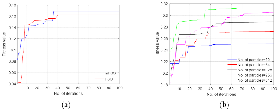
4.1. Particle Swarm Optimization

Particle Swarm Optimization (PSO), a relatively new family of algorithms that may be used to find optimal or near-to-optimal solutions. It is an optimization technique that provides an evolutionary-based search result on numerical and qualitative problems. It optimizes a problem by iteratively trying to improve a candidate solution. It is inspired by group behaviors in wildlife, for example, bird flocks, honeybees, ant colonies, and fish schooling.

In PSO, all particles are randomly initialized with velocity and position, and each particle keeps finding a candidate solution. Then, in each iteration, the velocity and position of each particle are renewed based on information about the previous velocity, the best position ever occupied by the particle, which is known as a personal influence, and the best position ever occupied by any particle in the swarm, known as a social swarm or global swarm. The mathematical formulations are as follows.

Let, assume the number of the particle is P, D denoting the dimensionality of a particle, and N stands for the iteration number. For any ith particle, position and velocity vector can be represented as $x_i$ and $v_i$, respectively. For standard PSO algorithm, there are two kinds of cost values, i.e., $p_{i,\hspace{0.17em}best}$ for the individual best value of one particle, and global best value $g_{best}$ of all particles, which can be written as Equations (25) and (26):

$$p_{i,best}=\hspace{0.17em}{p}_{i1,best},p_{i2,best},p_{i3,best},\dots ,p_{iN,best}$$

(25)

$$g_{best}=\hspace{0.17em}{g}_{1,best},g_{2,best},g_{3,best},\dots ,g_{N,best}$$

(26)

After determining the two cost values, the velocity and position of each particle in each dimension are renovated by using Equation (27) [1]:

$$\begin{gathered} v_{ij}\left(k+1\right)=w{v}_{ij}\left(k\right)+n_1{r}_1\left(p_{i,best}-x_{ij}\left(k\right)\right)+n_2{r}_2\left(g_{best}-x_{ij}\left(k\right)\right) \\ {x}_{ij}\left(k+1\right)=x_{ij}\left(k\right)+v_{ij}\left(k+1\right). \end{gathered}$$

(27)

In Equation (27), $r_1$ and $r_2$ denoting the random values between 0 and 1, w is the inertia coefficient which reflects the influence of the velocity in the previous iteration on the current iteration. $n_1$ and $n_2$ are self-cognitive and social cognitive values, which indicate the inheriting abilities from the particle itself and the whole swarm. Pseudocode for dynamic fitness function using PSO can be shown in Algorithm 1.

Algorithm 1: Pseudocode for Dynamic Fitness Function using PSO.

Initialize cell SAI values; while (CAC is not satisfied) { set monitoring UAV number = $N_{MDr}$; for j = 1:$N_{MDr}$ { set iteration number = $N_{iter}$; set particle number = $N_{par}$; for k = 1:$N_{iter}$ { for t = 1:$N_{par}$ { randomly initialize $x_t$ and $v_t$; initialize $P_{i,best}$ = $x_t$, $g_{best}$ = $x_{N_{par}}$; Update $x_t$ and $v_t$ using (26); Compute the fitness value of $x_t$ using (3) to (23); If($(fitness\left(x_t\right)>fitness\left(P_{i,best}\right))$ {$P_{i,best}=x_t$;} If($(fitness\left(P_{i,best}\right)>fitness\left(g_{best}\right))$ { $g_{best}=P_{i,best}$; $dynamic\_fitness=fitness\left(g_{best}\right);$ } } } update SAI value using Bresenham algorithm; } evaluate collisions among multiple UAVs.

4.2. Bresenham Algorithm

Bresenham’s line algorithm is a line drawing algorithm to form a close approximation to a straight line between two points by determining the points of an n-dimensional raster. This algorithm is named after Jack Elton Bresenham who developed it in 1962 at IBM [38]. This algorithm is a well-known earliest developed algorithm in the field of computer graphics. It is used for scan converting a line and involves only sixteen-bit integer addition, subtractions, and multiplication operations. The original algorithm extension can be used for drawing circles. In this method, the next point selected is the one that has the least distance from the true line. It can be also called an incremental error algorithm [39]. Some other algorithms are also frequently used in modern computer graphics because they can support antialiasing. Since this algorithm has been used for drawing a line from one particular point to another, we used this technique to ensure we conducted surveillance for the whole operational area. When this algorithm draws a line from one point to another point, it marks up the pixel or points between those two points. Similarly, in our implementation, when monitoring drones surveille from one waypoint to another waypoint (waypoints of best-paths which are generated through PSO algorithm), it made the cell SAI value zero to the corresponding cell SAI values. By making the cell SAI value to zero, we ensured that those cells have been visited by the monitoring drones. Therefore, in the next flight time, monitoring drones were not required to surveille those cells as there was a focus on surveilling the remaining cells. Therefore, we ensured the whole surveillance of the operational area and avoided the repetition of previously surveilled cells.

The working procedure of the Bresenham Algorithm can be described as follows. Once a point is chosen at any step, the next point is,

• Either the one to its right (lower-bound for the line)
• On top, it is right and up (upper-bound for the line).

Bresenham’s algorithm is used to implement the construction of a straight-line trajectory [40]. Assuming the initial position is (x₁, y₁), the direction to follow is the endpoint (x_end, y_end), which is given by the straight line. The objective of the algorithm is to construct a straight line approximately by deriving the sequence of positions in the grid. This is achieved by moving at each step to the next position along the x-axis (i.e., from x_i to x_i+1) and then by selecting y_i or y_i+1 which is the closest coordinate to the line. The points in the grid are indicated as (x_i, y_i) where i is used for index labeling the points in the grid. Thus, the y coordinate value at each step in the grid is chosen. While a decision parameter p_i is chosen, the calculation is done for each time step.

The algorithm is described as follows:

• Start from the two-line, starting point (x₁, y₁) and endpoint (x_end, y_end) and then calculate the constants where $\Delta x=\left(x_{end}-x_1\right)$ and $\Delta y=\left(y_{end}-y_1\right)$.
• Calculate the first value of the decision parameter by using the equation:

  $$p_0=2\Delta y-\Delta x.$$

  (28)
• For each value of x_i along the line, check the following condition, if p_i < 0, the next point needs to be selected as (x_i+1, y_i) and:

  $$p_{i+1}=p_i+2\Delta y.$$

  (29)
• Otherwise, the next point to be selected is (x_i+1, y_i+1) and:

  $$p_{i+1}=p_i+2\Delta y-2\Delta x.$$

  (30)

Repeat the steps until the set destination i.e., (x_end, y_end) is reached

The pseudocode of the Bresenham algorithm is given in Algorithm 2:

Algorithm 2: Pseudocode of Bresenham Algorithm.

Initialize waypoints and load variables x1, x2, y1, y2, d, i1, i2, dx, dy; Current waypoints = x1, y1, Next waypoints = x2, y2; Calculate $d_x$ = x2 − x1, $d_y$ = y2 − y1, d = dy/dx; Calculate $i_1$= 2 ∗ dy, $i_2$ = 2 ∗ (dy − dx), d = i1 − dx; Consider (x, y) as starting point and (xend, yend) as maximum possible value of x and y; If $d_x<0$ { $\mathrm{x}=x_2$; $\mathrm{y}=y_2$; $x_{end}$ = $x_1$; } If $d_x>0$ { $\mathrm{x}=x_1$; $\mathrm{y}=y_1$; $x_{end}$ = $x_2$; } Generate point at (x, y) coordinates; Check if the whole line is generated; If $x\ge x_{end}\hspace{0.17em}\left\{\mathrm{stop}\right\}$; Calculate coordinates of the next point; If $d<0\hspace{0.17em}\{d=d+i_1\}$; If $d\ge 0\hspace{0.17em}\{d=d+i_2;increment\hspace{0.17em}\hspace{0.17em}y=y+1\}$; Increment x = x + 1; Draw a point of latest (x, y) coordinates; Go to line 19; End of Algorithm.

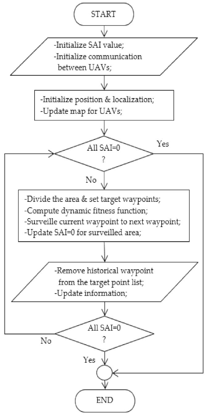
4.3. Distributed Path Planning for Multi-UAVs

The implementation of the proposed method is as follows: At the very beginning, it initializes the SAI values of each cell and establishes a connection among the monitoring drones. After establishing the connections, they share their positions and locations among themselves. We assumed that drone uses vision-based techniques and communication are done by mobile Ad-hoc manner [1].

After establishing the connections, the monitoring drone starts checking the area by using the historical data of SAI values. If they are not all covered, they divide the whole operation area into different important levels accordingly. Then, the target points are set to surveillance priority according to a different important area. Then, individual trajectories are generated for each monitoring drone, and objective and constraints value will be checked for the feasibility of the paths. The monitoring drones keep communicating with each other continuously and make the trajectory for the whole coverage.

Bresenham’s line drawing algorithm was used in this work to check if all the targeted areas have been visited or not. When the monitoring drone flies from a one-way point to another waypoint, the SAI value of those cells becomes zero (0). Therefore, after visiting all the surveillance areas, it will check all the areas have been covered or not; if not, then it will make the new path planning to cover all the areas. Thus, we could ensure the surveillance of the whole operational area. The implementation step of distributive path planning, including Pseudocode and Flowchart (Figure 2) for the whole operational scenario, as shown in Algorithm 3, and Figure 1, respectively.

Algorithm 3: Pseudocode for Distributed Path Planning

Initialize SAI value of each cell; Initialize communication between UAVs; Declare Number of UAVs = NUAV; Locate UAVs in the map; Initialize position and localization; Update map for UAVs; While $SAI\ne 0$ { for k = 1: NUAV { Divide the area according to the importance; Set target waypoints (bestpath) need to be covered; Compute dynamic_fitness function; Generate bestpath for all UAVs; for i = 1: bestpath { Update Swarm of UAVs; Surveille from current waypoint to next waypoint; Remove historical waypoint from target point list; } } Update and check, all SAI = 0 for the surveilled area; } Generate collision-free trajectory for multiple UAVs.

5. Simulation Results and Discussion

In this paper, we developed a Matlab-based operational environment to evaluate the working performance of the proposed multi-UAV path planning system. The main simulation parameters are listed in

Table 2. Simulation parameters.

Parameters	Symbols	Values
Grid Side (2-D environment)	-	20$\hspace{0.17em}\times \hspace{0.17em}$20
Operational Space (3-D environment)	-	$20\times 20\times 1.5$
Number of drones	ND	4
Drone unit power	Pw	20
Monitoring drone speed	v	10 m/s
Number of particles	Npar	32, 64, 128, 150, 256, 512
Number of iterations	Niter	100
Minimum safe distance	dmin	0.2 m
Initial SAI value	$v_{cellx}^{ini}$	4 to 10
Initial environment risk	$r^e$	1–5

.

For PSO algorithm parameter setting, the authors in [41] suggested the value of important parameters, like inertia, is 0.7298 and both the cognitive value as 1.4960. The authors in [42] suggested that inertia value can be selected within the value range from 0.4 to 0.9 and optimal value can be achieved by trial and error methodology, where the cognitive value can be selected as 2.0. We conducted a simulation by using both values and found that the second parameter value set has the better result, in terms of our simulation parameters. Therefore, the resulting values of the parameter have been used in this paper. We demonstrate the comparison between conventional PSO and PSO with modified parameters (mPSO) in Figure 3a. The result shows that the fitness value of the proposed modified-PSO (mPSO) algorithm converges faster to a stable value as the number of iterations increases. In the simulation, mPSO achieved higher Fitness values in a much shorter period of time than the conventional PSO, which led UAVs to surveille full areas in a short period of time. As the fitness value is the major factor for our proposed trajectory planner, we compared PSO and mPSO for their fitness value, in terms of the convergence over the number of iterations. This is the reason why we followed mPSO for further experimentation. These parameter values of PSO and mPSO are given in

Table 3. Comparison between Conventional PSO and m-PSO.

Parameter Name	Conventional PSO	PSO with Modified Parameters (mPSO)
Inertia value	0.7298	0.8
Personal Cognitive value	1.4960	2.0
Social Cognitive value	1.4960	2.0

.

As we increased the number of particles, we observed an improvement in the dynamic fitness function. The observed improvement of the dynamic fitness function is shown in Figure 3b.

In the objective function designing, we had to consider the impact of energy consumption, flight risk estimation, and SAI value on each other, where all the values had been normalized. It was supposed to have the optimal flight path, which consists of less energy consumption and flight risk, and a higher SAI value. For this reason, we designed the function by considering energy consumption and flight risk with a minimum value, where the SAI value has to be the maximum value. Figure 4 represents the objective function value curve and total fitness values under EC, FRE, SAI, respectively, where the number of iterations is 100 and the number of particles is 150. It shows the trajectory optimization performance of the flight time, in terms of energy consumption, fight risk, and surveillance area importance. As the number of iterations increased, the energy consumption and flight risk minimized and maintained a stable value, while their surveillance area importance values maximized. From the simulation results shown in Figure 4, it is observed that the simulation begins with the last value achieved from the dynamic fitness function. As the number of iterations increased the energy consumption, flight risk, and SAI value converged quickly and gradually improved the performance of the dynamic fitness function. This ensured that at each iteration, the particles tried to minimize energy consumption and flight risk, while maximizing the SAI value, which proves the effectiveness of our proposed algorithm. The optimization performance of the path planner, in terms of energy consumption and flight risk estimation, can be expressed as a fitness function that indicates the effectiveness of path planning. Fitness function itself consists of two parts, (i) objective value, (ii) constraints value. An optimal path should not have any kind of constraints in its path planning, thus, all constraints should be zero. Figure 5a, demonstrates the effectiveness of our paths where all the constraints are zero. Figure 5b,c show the objective value, and total fitness value, respectively for the different part of fitness values in each waypoint.

The SAI weight value has an impact on the total fitness value. Therefore, to find the necessary optimal weight value for SAI we conducted various simulations, as shown in Figure 6. As the weight value of SAI was expected to be positive, we selected a wide range of positive values for our simulation. For a large value of the weight, the impact on EC, FRE, and SAI was less. Therefore, we selected the weight value from a minimal positive value. The weight values and corresponding impact on EC, FRE, and SAI, along with objective values, are shown in

Table 4. Objective value varying SAI weight value.

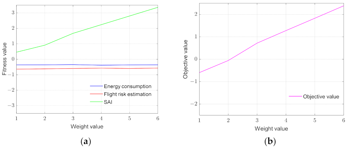
Weight Value	Energy Consumption	Flight Risk Estimation	Surveillance Area Importance	Objective Value
1	−0.3619	−0.6356	0.4597	−0.5978
2	−0.3577	−0.6186	0.9096	−0.0567
3	−0.3478	−0.5939	1.6792	0.7178
4	−0.3789	−0.5705	2.2389	1.2775
5	−0.3652	−0.5937	2.7986	1.8297
6	−0.3580	−0.5655	3.3583	2.3848

.

In our implementation, a full area coverage was based on distributed path planning. We considered two scenarios of full coverage, with overlapping, and without overlapping, respectively. In overlapping conditions, to cover the whole surveillance area, UAVs take so many steps that are known as waypoints. Sometimes, it takes very high computational time to complete the task. On the other hand, the second scenario is a non-overlapping condition, which requires less computational time and converges faster. To make the environment less complicated and faster and more convenient to converge, we only considered the second scenario, in this study, which involves path planning with the non-overlapping condition.

Figure 7a, shows the optimal paths, followed by UAV1, UAV2, UAV3, and UAV4 started from the GBS set as the starting point and denoted by a green rectangular box. After surveilling of the whole area, it again came back to the endpoint, marked as a yellow rectangular box. In Figure 7a, the red rectangle box represents the restricted areas where UAVs are not allowed to fly. With the edge cells having higher SAI value, UAVs need to surveille those edge areas first having level-3 importance, then the inner areas having level-2 priority, and the center having least priority as level-1. We gave the cell edge area more importance by considering that, generally when we design anything, we give more importance to the center as our valuable infrastructure is situated in the center. In that sense, edge areas received less importance, which may pose a great threat. Whenever any threats begin, they commence from the outside region first not from the inside area. Moreover, if we can prevent it earlier, before entering the sensitive area, we will be able to lessen the threat much. That is the reason why we gave cell edge more importance. We observed that the trajectories, generated for each flight time, avoid all the restricted areas and reach the destination safely after full coverage of the surveillance area.

Our operational area is based on a 3-D environment, while covering the distance from one waypoint to another waypoint, UAV made changes in the X, Y, and Z-axis. Altitude changes for all the UAVs during flight time are shown in

Table 5. Altitude changes of the UAVs.

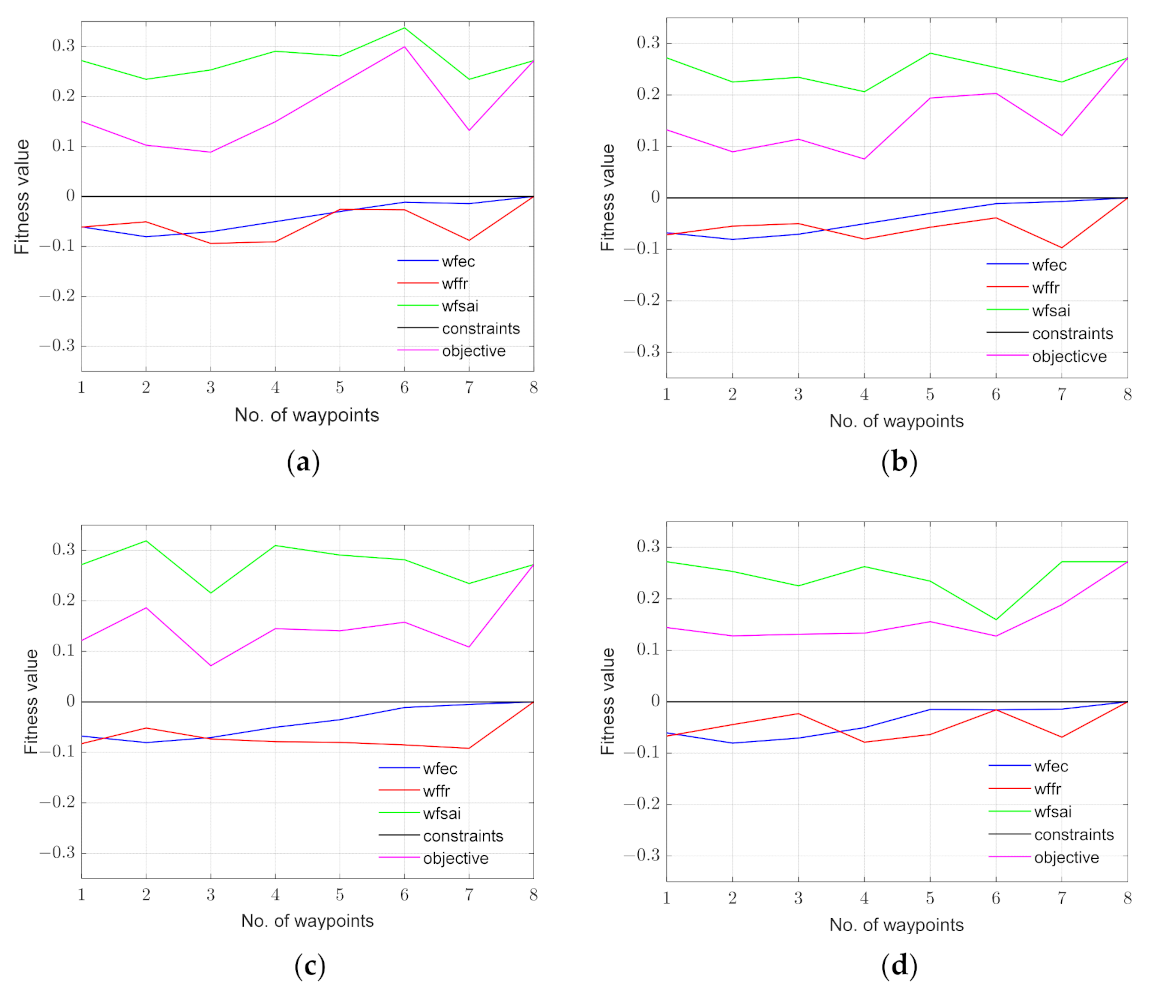
No. of Waypoints	Altitude (Meter)
	UAV1	UAV2	UAV3	UAV4
1	0.4827	0.4792	0.3403	0.5184
2	1.3508	0.3393	1.3211	0.8365
3	1.1563	0.9815	1.2727	0.4283
4	1.3724	0.2747	1.1685	0.9781
5	0.8549	0.8525	1.3761	0.0475
6	0.8316	0.1218	0.8848	0.1951
7	0.8528	0.0602	1.0310	0.5889
8	0.5366	0.5191	0.4815	0.5165

and the corresponding flight times for the UAVs can be seen in

Table 6. Flight chart of the UAVs.

UAV Number	Distance Covered in 2-D (Meter)	Time Required for 2-D (Second)	Distance Covered in 3-D (Meter)	Time Required for 3-D (Second)
1	3,152	315.2	3,159	315.9
2	3,155	315.5	3,164	316.4
3	3,184	318.4	3,195	319.5
4	3,052	305.2	3,056	305.6

. Figure 7b also shows that the ability of UAVs to decide to change in altitude and turning angle when hills or unstructured environment appear in path planning shows that our system has dynamic environment adaptability.

The proposed trajectory planner also ensures that the multiple UAVs do not collide with each other while surveilling. The respective Fitness values of all four UAVs for full coverage are shown in Figure 8.

In our simulation, the operating area was assumed to be 1 km × 1 km, with a per cell value of 50 m. During the surveillance, UAVs took off from the starting point and returned to the ending point. Table 6 shows the total distances covered by the UAVs and the necessary flight time for both 2-D and 3-D cases and it is observed that in a 3-D environment, UAVs cover more distance than in a 2-D environment. In our implementation, we assume that a UAV can cover up to four cells from a single location. As a result of this assumption, we can see that all of the UAVs have covered the entire operational region, except the restricted area, which is not allowed to be surveilled.

Distributed Path Planning for Multi-UAVs in the 2-D and 3-D environment for the larger-sized area is shown in Figure 9. To consider a larger size for our simulation we have selected a 30 × 30 grid size having the area of 3 km × 3 km (per cell 100 m). In our simulation where grid size was 20 × 20, each of the four UAV needs 8 waypoints to surveille the whole area. However, as the operational area size increased, the number of the required waypoints also increased; that is, 11 waypoints for each of the UAV.

6. Conclusions

In this paper, we proposed a distributed 3-D path planning for multiple UAVs, based on Particle Swarm Optimization with Bresenham Algorithm, to make an optimal trajectory for multiple UAVs. We introduced a multi-dynamic fitness function that has optimization indexes, such as energy consumption, flying risk, surveillance area importance (SAI), and UAV maneuverability. Moreover, we also obtained the optimal weight of SAI for an objective value to obtain dynamic fitness to generate a collision-free trajectory for multiple UAVs. To analyze the performance of the proposed optimal trajectory planner, we designed a dynamic fitness function mechanism with a cost function. The numerical results of experiments carried out in this research work show that the PSO, with Bresenham Algorithm, can be applied for multi-UAVs to surveille the whole area of interest by generating an optimal path. Currently, we carry out experiments for the swarm of four UAVs, and we evaluate feasibility, robustness, and dynamic environment adaptability for our three dimensions distributed trajectory planner to analyze the performance and effectiveness of the system. The simulation results prove that our proposals can perform a collision-free distributed trajectory planning for multiple UAVs to surveille the whole area of interest by flight time and flight distance optimized manner. For future work, we will consider an unstructured dynamic environment to perform three dimensions of distributed trajectory planning. We may apply our developed distributed trajectory planner to interface with the drone model for security purposes, to make a real-time application of multiple UAVs for full area surveillance under a dynamic environment.

References

- Teng, H.; Ahmad, I.; Msm, A.; Chang, K. 3D Optimal Surveillance Trajectory Planning for Multiple UAVs by Using Particle Swarm Optimization With Surveillance Area Priority. IEEE Access 2020, 8, 86316–86327. [Google Scholar] [CrossRef]
- Sheng, G.; Min, M.; Xiao, L.; Liu, S. Reinforcement Learning-Based Control for Unmanned Aerial Vehicles. J. Commun. Inf. Netw. 2018, 3, 39–48. [Google Scholar] [CrossRef]
- Yang, Q.; Yoo, S.-J. Optimal UAV Path Planning: Sensing Data Acquisition Over IoT Sensor Networks Using Multi-Objective Bio-Inspired Algorithms. IEEE Access 2018, 6, 13671–13684. [Google Scholar] [CrossRef]
- Zhan, C.; Zeng, Y.; Zhang, R. Energy-efficient data collection in UAV enabled wireless sensor network. IEEE Wirel. Commun. Lett. 2018, 7, 328–331. [Google Scholar] [CrossRef] [Green Version]
- Yang, L.; Qi, J.; Xiao, J.; Yong, X. A literature review of UAV 3D path planning. In Proceedings of the 11th World Congress on Intelligent Control and Automation, Shenyang, China, 29 June–4 July 2014; pp. 2376–2381. [Google Scholar] [CrossRef]
- Geraerts, R. Planning short paths with clearance using explicit corridors. In Proceedings of the IEEE International Conference on Robotics and Automation, Anchorage, Alaska, 3 May 2010; pp. 1997–2004. [Google Scholar]
- Yang, K.; Sukkarieh, S. Real-time continuous curvature path planning of UAVs in cluttered environments. In Proceedings of the 5th International Symposium on Mechatronics and Its Applications, ISMA 2008, Amman, Jordan, 27–29 May 2008; pp. 1–6. [Google Scholar]
- Cho, Y.; Kim, D.; Kim, D.S.K. Topology representation for the Voronoi diagram of 3D spheres. Int. J. CAD/CAM 2005, 5, 59–68. [Google Scholar]
- Musliman, I.A.; Rahman, A.A.; Coors, V. Implementing 3D network analysis in 3D-GIS. Int. Arch. ISPRS 2008, 37, 913–918. [Google Scholar]
- De Filippis, L.; Guglieri, G.; Quagliotti, F. Path Planning strategies for UAVs in 3D environments. J. Intell. Robot. Syst. 2012, 65, 247–264. [Google Scholar] [CrossRef]
- Carsten, J.; Ferguson, D.; Stentz, A. 3d field d: Improved path planning and replanning in three dimensions. In Proceedings of the 2006 IEEE/RSJ International Conference on Intelligent Robots and Systems, Beijing, China, 9–15 October 2006; pp. 3381–3386. [Google Scholar]
- Miller, B.; Stepanyan, K.; Miller, A. 3D path planning in a threat environment. In Proceedings of the 2011 50th IEEE Conference on Decision and Control and European Control Conference (CDC-ECC), Orlando, FL, USA, 12–15 December 2011; pp. 6864–6869. [Google Scholar]
- Masehian, E.; Habibi, G. Robot path planning in 3D space using binary integer programming. Proc. World Acad. Sci. Eng. Technol. 2007, 23, 26–31. [Google Scholar]
- Chamseddine, A.; Zhang, Y.; Rabbath, C.A. Flatness-based trajectory planning/replanning for a quadrotor unmanned aerial vehicle. Aerosp. Electron. Syst. IEEE Trans. 2012, 48, 2832–2848. [Google Scholar] [CrossRef]
- Borrelli, F.; Subramanian, D.; Raghunathan, A.U. MILP and NLP techniques for centralized trajectory planning of multiple unmanned air vehicles. In Proceedings of the American Control Conference, Minneapolis, MN, USA, 14–16 June 2006; p. 6. [Google Scholar]
- Hasircioglu, I.; Topcuoglu, H.R.; Ermis, M. 3-D path planning for the navigation of unmanned aerial vehicles by using evolutionary algorithms. In Proceedings of the 10th Annual Conference on Genetic and Evolutionary Computation, Atlanta, GA, USA, 12–16 July 2008; pp. 1499–1506. [Google Scholar]
- Kroumov, V.; Yu, J.; Shibayama, K. 3D path planning for mobile robots using simulated annealing neural network. Int. J. Innov. Comput. Inf. Control 2010, 6, 2885–2899. [Google Scholar]
- Scholer, F.; la Cour-Harbo, A. Generating approximative minimum length paths in 3D for UAVs. In Proceedings of the IEEE Intelligent Vehicles Symposium, Madrid, Spain, 3–7 June 2012; pp. 229–233.
- Pehlivanoglu, Y.V.; Baysal, O.; Hacioglu, A. Path planning for autonomous UAV via vibrational genetic algorithm. Aircr. Eng. Aerosp. Technol. Int. J. 2007, 79, 352–359. [Google Scholar] [CrossRef]
- Shahidi, N.; Esmaeilzadeh, H.; Abdollahi, M. Memetic Algorithm Based Path Planning for a Mobile Robot. In Proceedings of the International Conference on Computational Intelligence, Istanbul, Turkey, 17–19 December 2004; pp. 56–59. [Google Scholar]
- Foo, J.L.; Knutzon, J.; Kalivarapu, V. Path planning of unmanned aerial vehicles using B-splines and particle swarm optimization. J. Aerosp. Comput. Inf. Commun. 2009, 6, 271–290. [Google Scholar] [CrossRef]
- Cheng, C.T.; Fallahi, K.; Leung, H. Cooperative path planner for UAVs using ACO algorithm with Gaussian distribution functions. In Proceedings of the IEEE International Symposium on Circuits and Systems, ISCAS, Taipei, Taiwan, 24–27 May 2009; pp. 173–176. [Google Scholar]
- Xi, J.; Li, S.; Sheng, J.; Zhang, Y.; Cui, Y. Application of Improved Particle Swarm Optimization for Navigation of Unmanned Surface Vehicles. Sensors 2019, 19, 3096. [Google Scholar]
- Li, Y.; Chen, H.; Meng, J.E. Coverage path planning for UAVs based on enhanced exact cellular decomposition method. Mechatronics 2011, 21, 876–885. [Google Scholar] [CrossRef]
- Peng, H.; Shen, L.C.; Huo, X.H. Research on Multiple UAV Cooperative Area Coverage Searching. J. Syst. Simul. 2007, 19, 2472–2476. (In Chinese) [Google Scholar]
- Wu, Q.P.; Zhou, S.L.; Yin, G.Y. Improvement of Multi-UAV Cooperative Coverage Searching Method. Electron. Opt. Control 2016, 23, 80–84. [Google Scholar]
- Guo, Y.; Qu, Z. Coverage control for a mobile robot patrolling a dynamic and uncertain environment. In Proceedings of the Fifth World Congress on Intelligent Control and Automation, WCICA 2004, Hangzhou, China, 15–19 June 2004; Volume 6, pp. 4899–4903. [Google Scholar]
- Araujo, J.F.; Sujit, P.B.; Sousa, J.B. Multiple UAV area decomposition and coverage. In Proceedings of the Computational Intelligence for Security and Defense Applications (CISDA), Singapore, 16–19 April 2013; pp. 30–37. [Google Scholar]
- Xuan, Y.B.; Huang, C.Q.; Wu, W.C. Coverage search strategies for moving targets using multiple unmanned aerial vehicle teams. Syst. Eng. Electron. 2013, 35, 539–544. [Google Scholar]
- Belkadi, A.; Ciarletta, L.; Theilliol, D. UAVs team flight training based on a virtual leader: Application to a fleet of Quadrotors. In Proceedings of the 2015 International Conference on Unmanned Aircraft Systems (ICUAS), Denver, CO, USA, 9–12 June 2015; pp. 1364–1369. [Google Scholar]
- Belkadi, A.; Ciarletta, L.; Theilliol, D. UAVs fleet control design using distributed particle swarm optimization: A leaderless approach. In Proceedings of the 2016 International Conference on Unmanned Aircraft Systems (ICUAS), Arlington, VA, USA, 7–10 June 2016; pp. 364–371. [Google Scholar]
- Belkadi, A.; Abaunza, H.; Ciarletta, L.; Castillo, P.; Theilliol, D. Distributed Path Planning for Controlling a Fleet of UAVs: Application to a Team of Quadrotors * *Research supported by the Conseil Regional de Lorraine, the Ministére de L’Education Nationale, de l’Enseignement Supérieur et de La Recherche, and the National Network of Robotics Platforms (ROBOTEX), from France. IFAC-Pap. OnLine 2017, 50, 15983–15989. [Google Scholar] [CrossRef]
- Belkadi, A.; Abaunza, H.; Ciarletta, L.; Castillo, P.; Theilliol, D. Design and Implementation of Distributed Path Planning Algorithm for a Fleet of UAVs. IEEE Trans. Aerosp. Electron. Syst. 2019, 55, 2647–2657. [Google Scholar] [CrossRef]
- Golzari, S.; Zardehsavar, M.N.; Mousavi, A.; Saybani, M.R.; Khalili, A.; Shamshirband, S. KGSA: A Gravitational Search Algorithm for Multimodal Optimization based on K-Means Niching Technique and a Novel Elitism Strategy. Open Math. 2018, 16, 1582–1606. [Google Scholar] [CrossRef] [Green Version]
- Zheng, C.; Li, L.; Xu, F.; Sun, F.; Ding, M. Evolutionary route planner for unmanned air vehicles. IEEE Trans. Robot. 2005, 21, 609–620. [Google Scholar] [CrossRef]
- Cabreira, T.; Brisolara, L.; Ferreira, P., Jr. Survey on coverage path planning with unmanned aerial vehicles. Drones 2019, 3, 4. [Google Scholar] [CrossRef] [Green Version]
- Noonan, A.; Schinstock, D.; Lewis, C.; Spletzer, B. Optimal Turning Path Generation for Unmanned Aerial Vehicles (No. SAND2007-3152C); Sandia National Lab. (SNL-NM): Albuquerque, NM, USA, 2007. [Google Scholar]
- Bresenham, J.E. Algorithm for computer control of a digital plotter. IBM Syst. J. 1965, 4, 25–30. [Google Scholar] [CrossRef]
- Koopman, P., Jr. Bresenham Line-Drawing Algorithm; Fourth Dimension: North Kingstown, RI, USA, 1987; pp. 12–16. [Google Scholar]
- Rashid, A.T.; Ali, A.A.; Frasca, M.; Fortuna, L. Path planning with obstacle avoidance based on visibility binary tree algorithm. Robot. Auton. Syst. 2013, 61, 1440–1449. [Google Scholar] [CrossRef]
- Roberge, V.; Tarbouchi, M.; Labonte, G. Comparison of parallel genetic algorithm and particle swarm optimization for real-time UAV path planning. IEEE Trans. Ind. Inf. 2013, 9, 132–141. [Google Scholar] [CrossRef]
- Jordehi, A.R.; Jasni, J. Parameter selection in particle swarm optimization: A survey. J. Exp. Theor. Artif. Intell. 2012, 25, 527–542. [Google Scholar] [CrossRef]