Evolution of Situated and Abstract Communication in Leader Selection and Borderline Identification Swarm Robotics Problems

Abstract

The design of robust yet simple communication mechanisms, that allow the cooperation through direct interaction among robots, is an important aspect of swarm robotics systems. In this paper, we analyze how an identical continuous-time recurrent neural network (CTRNN) controller can lead to the emergence of different kinds of communications within the swarm, either abstract or situated, depending on the problem to be faced. More precisely, we address two swarm robotics tasks that require, at some extent, communication to be solved: leader selection and borderline identification. The parameters of the CTRNN are evolved using separable natural evolution strategies. It is shown that, using the same starting conditions and robots’ controllers, the evolution process leads to the emergence of utterly diverging communications. Firstly, an abstract communication, in which the message carries all the information, results from evolution in the leader selection task. Alternatively, a purely situated communication, meaning that only the context is communicative, emerges when dealing with the borderline identification problem. Nonetheless, scalability and robustness properties are successfully validated.

1. Introduction

Swarm robotics (SR) [1] is the research field that, combining aspects of artificial intelligence and robotics, studies the use of many simple distributed robots that collectively cooperate in order to solve complex tasks. The tasks addressed by swarm robotics can be either intrinsically collective problems, that can uniquely be solved through interaction, or single agent problems whose results can be boosted in multi-agent setups. SR is widely inspired by how biological swarms work in nature [2], exposing the emergence of complex collective behaviors from local interactions. Some examples remarkably recurrent in swarm robotics are ant colonies, bee colonies, flocks of birds, fish schools or slime molds, among others. In [3], the authors defined a set of conditions that a robotics system must fulfill in order to be considered a swarm robotics system: Autonomy, large swarm sizes, homogeneity, inefficiency and simplicity of single agents, local communication and sensing of the environment. Moreover, apart from efficiency in solving the task, scalability, robustness and flexibility are highly desirable properties in SR systems (see [3]).

In contrast to behavior-based design methods, automatic design methods find suitable robot’s controllers through an optimization process. The most important and widely used example of automatic design method is Evolutionary Robotics (ER) [4], and in particular, Evolutionary Algorithms (EA) to evolve the parameters of Artificial Neural Networks (ANN). The optimization of ANN parameters by means of evolutionary computation is called neuroevolution, see e.g., [5]. Nonetheless, the use of Recurrent Neural Networks (RNN) is of special interest in swarm robotics. The main reason is that they allow action generation not only based on current stimuli being measured but also based on past experience and events. Specifically, Continuous-Time Recurrent Neural Networks (CTRNN), see [6], have been employed as neuro-controllers in multiple works [7,8,9,10]. In [7], a CTRNN is evolved using a generational EA for the flocking of a swarm. They designed a fitness function that reflects cohesion, separation and alignment of the swarm, as in Reynolds’ rules. Tuci et al. [8] also optimize CTRNN controllers using an EA. In this case, they address a foraging problem, with a single nest and a single food area, in which robots have to decide whether they assume the role of foraging or nest patrolling. Moreover the task that they define imposes role switching within simulation to be completed correctly. Gutiérrez et al., proposed in [9] the evolution of CTRNNs using a generational genetic algorithm for the task of heading alignment of robots. The study is firstly analyzed in simulated environments and validated with real robots. In [10] the authors use a simple EA with roulette wheel selection and a CTRNN controller in order to solve the problem of cooperative transportation of heavy objects. The works listed above, in the context of evolutionary computation tools applied to the optimization of ANNs, are either Genetic Algorithms (GA) or Evolutionary Algorithms (EA) [11]. Other algorithms from evolutionary computation have also been employed in swarm robotics and collective robotics, such as differential evolution [12] or neuroevolution of augmenting topologies (NEAT) [13,14]. Besides, a family of algorithms that has gained research interest in the context of single agent controllers are Natural Evolution Strategies (NES) (see [15]). NES algorithms have recently proved to be competitive alternatives to deep reinforcement learning, tested in known benchmark problems such as Atari games or humanoid locomotion (see [16,17]). In NES, the population individuals are randomly sampled from a search distribution whose parameters are optimized in order to maximize the expected fitness (see Section 3.3), following the natural gradient direction. However, up to our knowledge, NES algorithms have not been applied to the field of swarm robotics yet. In this paper we explore the use of Separable Natural Evolution Strategies (SNES, see [18]), in order to evolve CTRNN neural controllers for different tasks.

Another critical design step in swarm robotics is the communication mechanics of the group. Communication within the swarm refers to any kind of interaction among robots in which information about states, actions or intentions of agents is shared across the swarm. According to [19], inter-agent communication in swarm robotics can be split into: Stigmergy, Interaction via state and Direct communication. Additionally, a different division can be provided if the communication technology is considered. Although not very common, long range communications, based on RF systems, have been used in swarm robotics when direction awareness is not an issue and long range global communication is required (see [20,21,22]). Middle range communication has also been addressed by means of sound (e.g., [23]) using speakers and microphones to produce and capture sound beeps. In both options, several of the exposed studies break the principle of locality presented at the beginning of the section. Therefore, minimal and short range communications are typically desirable in swarm robotics. For this type of communications, infrared (IR) technology is commonly employed (see [24]). IR sensors and emitters can be used for both distance estimation to solid objects [10,13,25,26], direct communication [27] or both [9]. Apart from its short coverage, IR technology presents several issues such as interferences, ambient light distortion, communication death zones, impossibility to send and receive at the same time or low data rates (see [25,28] for further details). However, it equally provides numerous advantages that make IR technology highly suitable for local communication in swarms of robots. Firstly, it is highly inexpensive and extremely low consuming, which, provided that swarm sizes can be arbitrarily large and individual robots are notably simple, are utterly desirable features in swarm robotics. Moreover, it allows a directionality awareness in the communication, as in-board IR communication in mobile robots is equipped with a set of receiver and emitters surrounding the robot perimeter. The knowledge of the direction from where neighboring robots are interacting with the agent is highly desirable in most applications and, more importantly, indispensable in many cases. Generally speaking, IR communication fulfills all previously exposed requirements for swarm robotics.

Another distinction can be highlighted in the case of semantics. Essentially, we can differentiate between direct communication semantics and codes that are handcrafted by the researcher and communication semantics that arise from automatic controller design methods (e.g., ER). In the latter scenario, it is said that communication emerges. Clearly, the researcher still has to design and establish the communication means and resources, albeit the semantics and the information relevant to the emerged communication is a result from optimization processes. Within this context, the taxonomy previously described according to [24] can be reformulated as follows (see [29]):

-

Abstract communication: is a type of communication in which only the message content carries information. The environmental context associated to the message is either not processed or not relevant in the emerged communication. See e.g., [30,31] and some of the experiments of [32].

-

Situated communication: refers to communication scenarios in which both the message content and its corresponding environmental context carry information within the communication. Environmental context can be, for instance, the signal strength from which the distance can be estimated or the direction from where the message was received. Some examples of situated communication are [9,33].

Another important question when designing communication systems in SR, guided by an evolution process, is whether it is possible or not to solve remarkably different tasks using the same robot controller. Moreover, can evolution lead to the emergence of different communication semantics depending on the task to be solved? In this paper, we address these questions. More precisely, the main motivation of this study is to assess if, using evolutionary computation, it is possible to achieve the emergence of opposed communication semantics (e.g., situated and abstract semantics) depending on the task to be solved and using the same neural controller architecture, with different optimization trajectories. In order to verify this concern, we propose two independent swarm robotics problems that require, at first sight, different communication semantics. The tasks are the election of a single leader of a swarm of static robots and the identification of the shape or borderline of a swarm of static robots. It can be expected beforehand that an abstract communication emerges when solving the leader selection problem. Alternatively, the borderline identification task requires, a priori, context information in order to be fulfilled. We consider that the proposed tasks are remarkably suitable benchmark experiments, in order to validate the previously mention hypothesis of communication emergence, due to the following reasons: (i) their successful completion requires communication, (ii) the required semantics of both problems are expected to be different and (iii) both tasks can be addressed using the same artificial neural network as robot’s controller (because the robot sensors and actuators are common to both experiments). Thereafter, the main contributions of this paper are the following:

-

We analyze and successfully verify that the same CTRNN controller model, evolved using separable natural evolution strategies, can lead to the emergence of different kinds of communications, either abstract or situated, depending on the problem to be faced. Specifically, we validate the previous statement for the tasks of leader selection and the borderline identification in a swarm of simulated static robots.

-

A minimal communication system, at disposal of the robots’ neural network, is proposed for solving the experiments and validating the hypotheses. The communication system allows robots to communicate directly, using an a priori meaningless message, or indirectly, by means of the corresponding environmental context information.

-

Apart from observing the communication semantics that emerge as a result of evolution in the proposed tasks, the resulting solutions are subject to a scalability and robustness analysis. In both cases, the obtained swarm robotics system fulfills both properties up to a considerable limit.

-

SNES algorithm is used to evolve the parameters of the neural controllers. Up to our knowledge, NES algorithms have not been applied to the field of swarm robotics, and, even though an exhaustive comparison should be carried out in the future, they are a noticeable alternative to other more widely explored automatic design methods in SR.

The remaining of the document is structured as follows. Section 2 provides a review of the related work. Additionally, Section 3 explains the simulated robots, the designed minimal communication system, the robot’s neural controller that maps stimuli to actions and the evolution process employed to optimize the controllers. Thereafter, Section 4 describes the proposed tasks to be solved. The results obtained after evolution are exposed in Section 5. Section 6 concludes the paper. Finally, the source code developed and used for this paper is available at https://github.com/r-sendra/SpikeSwarmSim accessed on 22 Janunary 2021.

2. Related Work

The first experiment that is considered is the leader selection and preservation in a swarm of static robots. The leader selection is an interesting problem in swarm robotics as the existence of a leader of the group, or from a more general perspective different assigned roles in the swarm, eases the resolution of multiple collective tasks, such as flocking [34,35], foraging [8], coordinated movement [36] or goal navigation [37] among others. The election of a swarm leader has been treated in several works [27,30,32,38]. Firstly, the leader selection procedure in [38] avoids the usage of direct communication among robots as it only employs the positions of other agents in the neighborhood. A robot becomes a leader whenever all the other robots in its vicinity lie on the same quadrant, considering the robot’s position as the origin of coordinates. In [30], the authors designed a voting algorithm based on local communication in a static swarm for the leader election, among other cooperative tasks. The results of their experiments successfully show consensus in the selection in most cases. Alternatively, one of the multiple experiments in [32] is the leader election. They employ Wave Oriented Swarm Paradigm (WOSP) techniques in order to trigger the emergence of collective behaviors, such as leader election, with local binary information exchange. The controllers are also handcrafted as outstandingly simple and compact finite state machines. Neither evolution nor neural controllers are explored in these papers. On the contrary, in [27], the leader selection and role allocation problems are faced using neural controllers and evolutionary computation. The swarm members communicate locally through a communication system and a robot can assume the role of leader by directly maximizing its communication output. In contrast with [27], in our study, we decouple CTRNN outputs for elaborating the communication message and claiming the leadership. Thus, the fitness function does not directly promote or reward the use of the communication channel.

The borderline identification of a swarm is a relevant problem in the context of collective tasks such as flocking, aggregation or shape formation. The awareness of the limits of the swarm can refine these tasks and potentially aid the avoidance of swarm disconnection. Additionally, the identification of the swarm shape can be harnessed for the estimation of areas (e.g., estimation of the burned area in forest fires). Varughese et al. [32] have treated the problem of boundary identification in the context of swarm robotics. They use minimalistic robot behaviors and binary communication using Wave Oriented Swarm Paradigm (WOSP).

Even though the tasks that are addressed and solved in this paper are remarkably important, the main motivation and contribution of this study is the following. We successfully verify that the same CTRNN controller model, optimized using evolutionary computation, can lead to the emergence of different kinds of communications, either abstract or situated, depending on the problem to be faced. In the case of the leader election problem, an abstract communication emerges while purely situated semantics arise in the case of the borderline identification task. The authors in [39] also addressed this problem, applied to other SR experiments. They compare the optimization of Probabilistic Finite State Machines (PFSM) and evolutionary algorithms applied to ANN in three different tasks. In both algorithms, the robots are endowed with the capability of broadcasting and receiving messages, whose semantics are initially undefined. They also evolved artificial neural networks using an evolutionary algorithm and the resulting solutions are compared with the behavior and communication of the optimized PFSMs. They report that the optimization of PFSM controllers can generate diverse message semantics in response to the problem to be solved, albeit the emergence of communication was not reached through their evolution process.

3. The Robots and the Communication

The simulated environment is a 10 m × 10 m square area where the robots of the swarm are placed. The set of robots belonging to the environment is denoted as $\mathcal{R}$ and, hereafter, we refer to a generic robot as $r\in \mathcal{R}$. Robots are modelled as static point particles, represented by a position ${\mathbf{x}}_r$ and a time dependent heading orientation ${\theta }_r\left(k\right)$. Owing to the fact that the simulated robots are static and their maximum communication range is about 80 cm (see Section 3.1), we consider that a 10 m × 10 m environment is large enough. More precisely, these dimensions allow the allocation of, at least, swarms of 50 static robots of 10 cm radius, while maintaining inter-robot distances in the range 30–80 cm. The simulated robots of the experiments treated in this paper are equipped with IR transmitters and receivers. IR transmitters and receivers allow the communication and interaction among agents in order to solve the proposed tasks. Alternatively, a LED actuator is used by the robots to notify their actions. The robots’ controller, responsible for the mapping of the measured stimuli to actions, is based on a continuous-time recurrent neural network (see Section 3.2) evolved using separable natural evolution strategies (see Section 3.3).

3.1. The Minimal Communication System

The communication system proposed in this paper, inspired by how mobile robots communicate using IR technology, is minimal because of the following main reasons:

-

The communication is local, with a remarkably small communication range. This means that two robots can communicate if their distance is lower than a threshold. The communication range is fixed to 80 cm (see [40]).

-

Only one message can be received at each time instant. This means that, regardless of the number of neighbors, the robot and, thus, the CTRNN is only aware of one neighbor at each simulation step.

-

The possible directions of message reception or the number of IR sectors are restricted to 4 sectors, highly complexifying the tasks.

-

The received context corresponds uniquely to the current received message.

Robots’ controllers are fed by the received message and its context and elaborate a new two-dimensional message to be isotropically broadcasted using the IR transmitter. Before transmitting the message, it is subject to a quantization mapping that converts the raw message content to one symbol in the set $\mathcal{C}$ (see Equation (1)).

$$\mathcal{C}={\left\{0,{\displaystyle \frac{1}{K-1}},\cdots ,{\displaystyle \frac{K-2}{K-1}},1\right\}}^M$$

(1)

where $M=2$ is the dimension of the message and $K=4$. This leads to 16 possible symbols in the communication. A symbol in $\mathcal{C}$ is randomly sampled assigning higher probabilities to the nearest symbols and lower probabilities to the symbols that are more distant. As proved in Section 5, 16 symbols are enough for the addressed applications and using the algorithms and techniques of this paper. It is shown how, even though there are 16 available symbols, the emerged communication uses, at most, only two of the symbols.

Alternatively, the IR receiver is sectorized, meaning that the coverage is split into equiareal sectors so that the agent can distinguish the orientation from where a message is sensed. We propose a minimal communication system and, consequently, the number of sectors is fixed to 4 in the tasks. This means that the reception orientation is discretized to ${\theta }_{RX}\in \{{\theta }_r,{\theta }_r+\pi /2,{\theta }_r+\pi ,{\theta }_r+3\pi /2\}$ radians. Two agents can directly communicate if their Euclidean distance is lower that 80$\mathrm{cm}$ and the misalignment is lower than $\pi /4$. By misalignment, we refer to:

$$misalignment=\pi -min\left\{|{\theta }_{RX}-{\theta }_{TX}|,2\pi -|{\theta }_{RX}-{\theta }_{TX}|\right\}$$

(2)

where ${\theta }_{RX}$ and ${\theta }_{TX}$ are the orientations of the sectors from where the message was received and transmitted, respectively.

Moreover, we propose the incorporation of a communication state ($MODE$ when referred as a binary variable) as follows: an agent can be either in send mode or in relay mode. Send mode means that the robot controller creates a novel message, based on the incoming message from its neighborhood, and broadcasts it to its vicinity. On the contrary, relay mode refers to broadcasting the input message sensed by the receiver. The commutation between these states will be performed by the agent controller. Moreover, a maximum number of hops is fixed so that old messages eventually stop from being relayed. Messages have an attached identifier of the robot that initially generated the message content in send mode. Therefore, an agent avoids receiving echoes of its own messages by filtering out incoming packets with its own identifier. As robots can only perceive one message per time cycle, a random selection among all the messages currently captured from all sectors is implemented. Moreover, only the context information corresponding to the chosen message if provided to the robot’s controller.

3.2. The Robot’s Controller

Continuous-Time Recurrent Neural Networks (CTRNN), see [6], are used as robot’s controllers in order to map sensed stimuli to actions. The neurons of the CTRNN are modelled as firing rate neuron models (see Chapter 11 in [41]), as a simplification of spiking neuron models assuming rate coding schemes. Firing rate model can be described as in Equations (3) and (4).

$$\tau {\displaystyle \frac{dv\left(t\right)}{dt}}=-v\left(t\right)+\mathrm{I}\left(t\right)$$

(3)

$$u\left(t\right)=\sigma \left(g\right(v\left(t\right)+\beta \left)\right)$$

(4)

Inspired from biological neuronal dynamics, $v\left(t\right)$ represents the time varying membrane potential of the neuron and $\mathrm{I}\left(t\right)$ is the instantaneous somatic current injected in the neuron as the contribution from all presynaptic neurons. Say, that the n-th neuron is connected to $N_{pre}$ presynaptic neurons and $N_{in}$ input nodes. Then, the somatic current injected to the n-th neuron is defined in Equation (5).

$${\mathrm{I}}_n\left(t\right)=\sum _{j=1}^{N_{pre}}{w}_{nj}{u}_j\left(t\right)+\sum _{i=1}^{N_{in}}{w}_{ni}^{\varphi }{\varphi }_i\left(t\right)$$

(5)

where $w_{nj}$ is the strength of the synapse with j-th presynaptic neuron and n-th postsynaptic neuron and $w_{ni}^{\varphi }$ is the strength of the synapse connecting input i to the n-th neuron model. Moreover, ${\varphi }_i\left(t\right)$ is the corresponding input stimulus signal. Additionally, $\tau$ is the membrane decaying time constant governing how rapidly $v\left(t\right)$ reaches stable fixed points in response to $\mathrm{I}\left(t\right)$. The second equation exposes the transformation of the membrane voltage into the variable $u\left(t\right)$ representing the neuron firing rate or activity. $\sigma$ is the sigmoid function (see Equation (6)) that maps membrane voltages into neuron activities.

$$\sigma \left(z\right)=\frac{1}{1+e^{-z}}$$

(6)

Besides, $\beta$ and g are constants that define neuron dynamical properties. In the case of $\beta$, it establishes the maximum voltage threshold that must be surpassed in order to produce non-zero firing rate $u\left(t\right)$. The constant g states how fast a neuron can switch from resting activity (null or scarce activity) to maximum firing rate. Note that large values will increase the slope of the sigmoid function within the linear region, producing a fast transition between minimum and maximum activities.

The precise CTRNN architecture used in this manuscript is presented in Figure 1. It is composed by a set of input nodes representing the stimuli vector, two hidden layers of 10 neurons each and a series of motor neuron ensembles, whose activities are decoded into actions. In swarm robotics, it is a common practice to design CTRNN controllers with 1 or, at most, 2 hidden layers (see e.g., [7,8,9,10]). This configuration is a good tradeoff between processing capabilities and simplicity of the robot’s controllers. It should be noticed that the latter property is critical in swarm robotics systems. Besides, adding more hidden layers would drastically increase the dimension of the search space and, consequently, it would highly complexify the optimization problem. Moreover, as demonstrated in [42], an artificial neural network with a single hidden layer and with sigmoid activations can approximate any continuous function in ${[0,1]}^n$, provided that the weights are correctly adjusted. The input stimuli vector is composed by the readings of the communication receiver, namely, the message ${\mathbf{m}}_{RX}\in \mathcal{C}$, the communication state ($MODE\in \{0,1\}$, 0 representing the relay mode and 1 denoting send mode) and the encoded reception orientation ${\theta }_{RX}$. The actions decoded from motor neurons’ activities are $a_{LED}\in \{0,1\}$, for turning on or off the robot’s LED, the new communication state ($MODE\in \{0,1\}$, with the same meaning as the input) and the elaborated message (${\mathbf{m}}_{TX}\in {[0,1]}^2$). As it can be observed, the actions corresponding to $a_{LED}$ and $MODE$ are decoded using the Heaviside function $\mathcal{H}$ with discontinuity at 0.5, while the message decoding is the identity function (no decoding).

The simulator experiments operate at two different time scales. k is the time variable of the environment, so that, at each time instant of k, the agents read the current partially observable state using their sensors and perform actions. On the contrary, t is the time variable at the neuronal dynamics time scale. Considering that the random selection of input messages produces a high frequency stimuli signal, it is reasonable to set the neuronal dynamics at a much faster time scale than the world dynamics. More specifically, such a discontinuous and high frequential input signal would preclude the reaching of stable attractors or state space trajectories. In general, the relation between time scales is:

$$t=\delta k,\delta >1$$

The action at each world time step is decoded using the activities of the motor neurons at instants $t=\delta k$ using the decoders of Figure 1. Similarly, the input stimuli is maintained constant in between sampling instants of the environment:

$$\mathit{\varphi }(t+1)=\mathit{\varphi }\left(t\right),\forall t\in [\delta k,\delta (k+1)-1),\forall k\in [0,\infty )$$

where $\mathit{\varphi }$ is the overall stimuli vector. In all the experiments, $\delta$ is set to 20 so that during each environment step, the CTRNN dynamics are updated 20 times. Considering a real hardware implementation of the controller, the $\delta$ steps of the CTRNN can be scheduled in between sensor and actuator executions when the microcontroller would be idle otherwise. We experimentally found that a value of $\delta$ of 20 is, as a first approach, a good tradeoff between computational complexity and CTRNN capabilities of reaching steady states or stable state space trajectories.

3.3. Separable Natural Evolution Strategies

The parameters of the CTRNN of the neural controller are evolved using natural evolution strategies (see [15]). Natural Evolution Strategies (NES) are a family of evolutionary computation algorithms that, instead of directly evolving the population of individuals or genotypes, it updates a parametrized search distribution that is used to sample genotypes. NES algorithms maximize the expected fitness with respect to the search distribution parameters, as in Equation (7),

$$\underset{\mathbf{\theta }}{\mathrm{argmax}}\left\{{\mathbb{E}}_{\mathbf{\theta }}\left[f\left(\mathcal{G}\right)\right]\right\}$$

(7)

where f is the fitness function evaluating genotypes $\mathcal{G}$. Genotypes are sampled from the search distribution, $\pi \left(\mathbf{\theta }\right)$ generically speaking (see Equation (8)).

$$\mathcal{G}\sim \pi \left(\mathbf{\theta }\right)$$

(8)

In particular, Separable Natural Strategies (SNES) are used in this paper to evolve the parameters of the CTRNN controllers. SNES (see [18]) is a natural evolution strategy specifically suitable when dealing with large dimensional problems, such as in neuroevolution. It restricts the search distributions to multivariate normal distributions with diagonal covariance matrix $\mathbf{\Sigma }=\sigma \mathbf{I}$, with $\sigma \in {\mathbb{R}}_{>0}^d$. Therefore, the parameters to be evolved are $\mu$ and $\sigma$, both of the same dimension d (genotype length).

$${\displaystyle \mathcal{G}=\left(\begin{array}{c}\widehat{\mathbf{w}}\\ \widehat{g}\\ \widehat{\tau }\\ \widehat{\beta }\end{array}\right)}$$

(9)

The genotypes (see Equation (9)) are vectors bounded in ${[0,1]}^d$ resulting from the vector concatenation of normalized synapse weights ($\mathbf{w}$), neuron gains ($\mathbf{g}$), time constants ($\mathbf{\tau }$) and biases ($\mathbf{\beta }$). In order to constrain the search space to the hypercube ${[0,1]}^d$, these variables are normalized as in Equation (10), fixing the corresponding upper and lower bounds of the variables. On the contrary, when converting genotypes to CTRNN phenotypes to be evaluated, the variables are inversely denormalized as in Equation (11).

$$\left.\begin{array}{c}\widehat{\mathbf{w}}={\displaystyle \frac{\mathbf{w}-w_{min}}{w_{max}-w_{min}}}\hfill \\ \widehat{g}={\displaystyle \frac{\mathbf{g}-g_{min}}{g_{max}-g_{min}}}\hfill \\ \widehat{\mathbf{\beta }}={\displaystyle \frac{\mathbf{\beta }-{\beta }_{min}}{{\beta }_{max}-{\beta }_{min}}}\hfill \\ \widehat{\mathbf{\tau }}={\displaystyle \frac{log(0.5·\mathbf{\tau })-{\tau }_{min}}{{\tau }_{max}-{\tau }_{min}}}\hfill \end{array}\right\}$$

(10)

$$\left.\begin{array}{c}\mathbf{w}=\widehat{\mathbf{w}}·(w_{max}-w_{min})+w_{min}\hfill \\ \mathbf{g}=\widehat{\mathbf{g}}·(g_{max}-g_{min})+g_{min}\hfill \\ \mathbf{\beta }=\widehat{\mathbf{\beta }}·({\beta }_{max}-{\beta }_{min})+{\beta }_{min}\hfill \\ {\displaystyle \mathbf{\tau }=2·{10}^{\widehat{\tau }·({\tau }_{max}-{\tau }_{min})+{\tau }_{min}}}\hfill \end{array}\right\}$$

(11)

It should be mentioned that the same phenotype is used as neural controller for all robots in the experiments (homogeneity principle of swarm robotics). Finally,

Table 1. Search space constrains of each of the denormalized optimization variables.

Variable	Min.	Max.
$\mathbf{w}$	−3	3
$\tau$	−1	0.75
$\beta$	−1.5	1.5
$g$	0.05	5

exposes the search space bounds of each variable vector subject to evolution. The $[-1,0.75]$ range of $\tau$ is mapped to $[2\times {10}^{-1},2\times {10}^{0.75}]=[0.2,11.25]$ seconds. Equivalently, this search space of time constants allows the existence of a variety of neuronal regimes. For example, low time constants allow the rapid reaction to abrupt changes in the input stimuli, while large time constants permit the formation of working memory at a much slower time scale.

In the tasks addressed in this paper, SNES algorithm is executed during 1000 generations with a population size of 100. Each genotype is evaluated in a total of 5 independent trials or episodes and each trial is composed by 300 simulation steps.

4. The Experiments

4.1. Experiment A: Leader Selection

The objective of the leader selection experiment is to find a cooperative behavior in which just a single agent claims the leadership of the group during the evaluation period. Robots can claim leadership by turning their LED on. Cooperative solutions resulting in the swarm leader being the same during consecutive time instants will be rewarded, trying to avoid unnecessary switching of the leadership. However, it is highly desirable to find a swarm behavior capable of reacting to leader fault or loss by selecting a substitute. In order to guide evolution towards this behavioral feature, a robot becomes faulty if it has been the unique leader for 50 consecutive simulation cycles. In this context, a faulty robot means that the agent can only relay input messages (it is always in relay mode) and it cannot claim leadership. As communication is still operative after failure, the swarm graph cannot be broken or disconnected due to leader fault. The size of the swarm or the number of robots in $\mathcal{R}$ is set to 10, albeit there is a post evolution scalability analysis assessing the task for different swarm sizes. At the beginning of each simulation episode, the robots’ position are randomly initialized with a random spatial graph initializer that guarantees that there are no isolated swarm members. Heading orientations are also randomly initialized.

The fitness function rewards two main aspects of the swarm behavior in this problem, namely, leader identification and its preservation. On the one hand, the instantaneous fitness score increases at each time step when there is uniquely one leader in the group. On the other hand, the reward rises proportionally to the number of consecutive time steps that the leadership has been assumed by the same robot. The fitness function at each simulation instant is exposed in Equation (12).

$$f_A(\mathcal{G},k)=\mathbf{w}{\left(k\right)}^{\top }{\mathbf{a}}_{LED}\left(k\right)$$

(12)

The vector ${\mathbf{a}}_{LED}\left(k\right)\in {\{0,1\}}^R$ gathers the LED actions performed by all the agents in the swarm at time step k, subject to genotype $\mathcal{G}$. Moreover, ${\mathbf{a}}_{r,LED}\left(k\right)$ is the scalar LED action of the robot r in the group (which is one of the components of ${\mathbf{a}}_{LED}\left(k\right)$). The vector $\mathbf{w}\left(k\right)$ is a credit assignment vector that represents the number of consecutive time steps that a robot has been the leader.

$$\mathbf{w}\left(k\right)=\left\{\begin{array}{cc}min\{\mathbf{w}(k-1)+0.1{\mathbf{a}}_{LED}\left(k\right),5\}\hfill & \begin{array}{c}\mathrm{If}\sum _{r\in \mathcal{R}}{\mathbf{a}}_{r,LED}\left(k\right)=1\\ \mathrm{and}{\mathbf{a}}_{LED}\left(k\right)={\mathbf{a}}_{LED}(k-1)\end{array}\hfill \\ \\ 0.1{\mathbf{a}}_{LED}\left(k\right)\hfill & \begin{array}{c}\mathrm{If}\sum _{r\in \mathcal{R}}{\mathbf{a}}_{r,LED}\left(k\right)=1\\ \mathrm{and}{\mathbf{a}}_{LED}\left(k\right)\ne {\mathbf{a}}_{LED}(k-1)\end{array}\hfill \\ \\ {(\underset{R\mathrm{times}}{\underbrace{0,\cdots ,0}})}^{\top }\hfill & \mathbf{Otherwise}\hfill \end{array}\right.$$

(13)

Specifically, Equation (13) describes the computation of $\mathbf{w}\left(k\right)$. Note that the components corresponding to activated LEDs are increased 0.1 up to a maximum of 5. This increment is only performed if there is only one leader (i.e., only one LED action to 1) and the current leader is the same as the previous one, as specified in the condition of the equation. Alternatively, if there is only one leader but it is not the same as the previous one (or there was not a leader) then the credit assignment is 0.1. Provided that none of the former conditions are fulfilled, the credit assignment vector is reset to zeros. With the meaning of $\mathbf{w}\left(k\right)$ in mind, we can resume the explanation of Equation (12). Clearly, the dot product $\mathbf{w}{\left(k\right)}^{\top }{\mathbf{a}}_{LED}\left(k\right)$ will be higher as the credit assignment of a leader grows. Moreover, if there is more than one leader (${\parallel {\mathbf{a}}_{LED}\parallel }_1$ > 1) then the fitness is zero because $\mathbf{w}$ becomes the zero vector.

The fitness score of an episode is computed as the temporal average of the instantaneous fitness $f_A$ value of each evaluation time step:

$$F_A={\displaystyle \frac{1}{T_E}}\sum _{k=1}^{T_E}{f}_A(\mathcal{G},k)$$

Finally, each genotype is evaluated in 5 independent trials so that multiple fitness samples are used to construct the final expected fitness estimate. The final estimate is the sample mean of the fitness values obtained in each trial.

4.2. Experiment B: Borderline Identification

Borderline or frontier identification of a swarm of robots is the problem of detecting which nodes in a cluster surround the others. Given a set of points P, the aim is to find the subset of these points $P_B$ such that there is a closed polygon joining all elements in $P_B\subset P$ whose area contains all the other points in $P\setminus P_B$.

This boundary is approximated, for randomly generated node distributions, using the alpha shape algorithm, as a generalization of convex hulls (see [43]). Figure 2 shows the alpha shape of a randomly generated set of 100 points with the parameter $\alpha =15$. We heuristically concluded that this value is suitable for our application. The borderline points ($P_B$) are those points belonging to the obtained alpha shape. The interior points are the remaining nodes in the swarm, that are not considered extremities. Only those agents belonging to the alpha shape of the swarm should identify themselves as borderline. Robots can identify themselves as borderline members by turning their LED on. At each simulation cycle, the experiment can be understood as a binary classification problem in which agents have to decide if they belong to the boundary or not. Alpha shape is used to generate target values that increase the fitness of the swarm if the classification is correct. In the experiment proposed here, the target alpha shape is the same during the entire simulation period because of the stationarity of the swam. In practice, the lack of a large number of points, in our case robots, leads to highly probable scenarios where the borderline polygon is not closed (for instance, a swarm forming a line or a V-shape). In this case, all the robots in the swarm would belong to the frontier ($P_B=P$). The swarm topology graph and the robot’s orientation are randomly initialized as in Experiment A.

At each time step, the instantaneous fitness function will be higher as the number of correct LED decisions increase. A correct decision means that either a borderline member activates its LED (true positive) or that an interior robot turns off its LED (true negative). Let ${\mathcal{R}}_B\subset \mathcal{R}$ be the subset of robots belonging to the swarm borderline or frontier (note that there is a bijective correspondence between the elements of ${\mathcal{R}}_B$ and $P_B$). On the contrary, the subset of robots belonging to the interior of the swarm is denoted as ${\mathcal{R}}_I=\mathcal{R}\setminus {\mathcal{R}}_B$. The instantaneous fitness function is displayed in Equation (14). The function has two terms that are combined as a product. The first term corresponds to the number of borderline robots successfully identified divided by the number of borderline members. The second part is the number of correct classifications of interior agents divided by the number of interior robots. $R_B$ and $R_I$ denote the cardinality of the sets ${\mathcal{R}}_B$ and ${\mathcal{R}}_I$, respectively.

$$f_B(\mathcal{R},k)={\displaystyle \frac{1}{R_B{R}_I}}\left(\sum _{r\in {\mathcal{R}}_B}{\mathbf{a}}_{r,LED}\left(t\right)\right)·\left(R_I-\sum _{r\in {\mathcal{R}}_I}{\mathbf{a}}_{r,LED}\left(t\right)\right)$$

(14)

From a different perspective, the terms measure separately the true positive rate (TPR) and the true negative rate (TNR) instead of computing directly the total accuracy of the swarm. This fitness breakup is principally performed because the number of borderline and interior agents ($R_B$ and $R_I$) are highly unbalanced in most of the random initializations of the swarm topology. This leads to naive and utterly suboptimal solutions in which all robots identify themselves as interior or borderline due to the high overall accuracy. As in all the experiments, the fitness score of a trial is computed as the average of the instantaneous fitness values of each time step:

$$F_B={\displaystyle \frac{1}{T_E}}\sum _{k=1}^{T_E}{f}_B(\mathcal{R},k)$$

Similarly, 5 trials are accomplished, computing the final expected fitness estimate as the sample mean of all the episode fitness scores.

5. Results

The behaviors evolved are exhaustively analyzed for each task. For each experiment, this section is structured considering the following blocks:

-

Behavior: The emerged behavior and the resulting performance are discussed. Several figures, showing the swarm actions and the goodness of the solution, are shown to demonstrate the performance.

-

Scalability: In each experiment, the behavior is assessed for different swarm sizes.

-

Robustness: Robustness is evaluated by means of introducing an alteration in the task at some point in time during the simulation.

-

Communication: The emerged communication is described for each problem. Principally, the relevant communication information is figured out, highlighting the type of communication that has emerged (e.g., situated or abstract communication).

In order to present the results in the previous items, tools from descriptive statistics are considered. More precisely, 50 independent trials with random initialization are executed and gathered into a dataset. Afterwards, the dataset with 50 samples is used to support most of the figures and results of the experiments.

Figure 3 illustrates the fitness evolution in each experiment. Figure 3a shows the fitness evolution in the leader selection task, while Figure 3b focuses on the borderline identification experiment. For each generation, it shows the sample mean fitness score (darker curves) and the maximum and minimum fitness values (upper and lower contours of the shadow areas).

5.1. Experiment A: Leader Selection

Behavior: We observed two stages during the evaluation process. Firstly, agents carry out a negotiation phase in order to select a leader. Essentially, all the robots claim the leadership at the beginning of the negotiation process by turing their LEDs on. Thereafter, each robot being the leader eventually turns off its LED in order to yield leadership to other members of the swarm. The negotiation process can be understood as a winner-take-all competition among agents, so that each potential leader inhibits the others through the communication system. Consequently, the winner of the negotiation, and thus the leader, is the robot whose LED remains turned on. The second phase of the behavior is achieved if an agent is the unique leader of the swarm or, at least, if it does not receive any communication information specifying the opposite. In such a situation, a stable solution is reached and remains still unless a perturbation is introduced in the system. Agents are aware of other robots claiming leadership by means of the communication system. The discussion on the emerged communication is retrieved and elaborated in detail later.

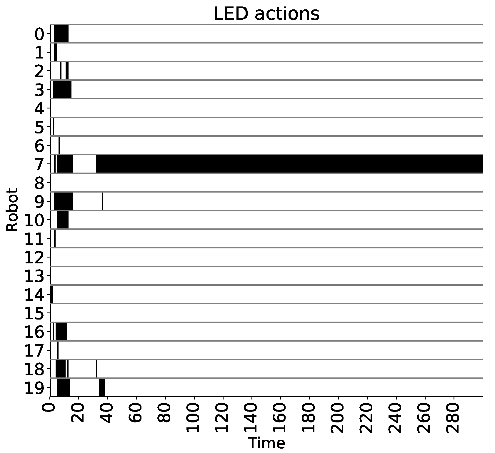
Figure 4 shows an example of the emerged behavior, displaying both negotiation and stable leader identification. It shows the LED actions of the agents in a swarm of size 20 as execution time elapses. Black bars indicate that the LED of the corresponding robot in the ordinate axis is turned on. There is no leader fault in this figure as it will be discussed in the robustness analysis below. The results of the figure closely resemble the behavior previously described. The negotiation stage, starting at time step 0 and concluding approximately at simulation cycle 40, exposes the winner-take-all process in which LED actions are constantly being deactivated. Nonetheless, the plot shows an unsuccessful negotiation scenario whereby all the robot LEDs are turned off and no leader is selected around time step 20. In such a case, it can be observed that another negotiation process, of much shorter duration, is initiated with less contestants. Finally, as a result of the second competition, a unique leader is identified and a stable behavior is settled until the simulation ends.

The results can be observed in Figure 5 from another perspective, using a different simulation trial. The figure illustrates different frames of a simulation of this experiment. The red balls represent robots whose LED is turned on and the blue balls show agents with deactivated LED. Only instants previous to time step 20 are shown. After this time instant, leader is settled and stable. The last resource to observe the behavior of robots within this task is provided as a video recoding the simulation (https://youtu.be/ahBlVf9jAbw accessed on 9 Janunary 2021).

Scalability: The scalability of the solution is assessed by simulating the experiment with different swarm sizes. Moreover, instead of depicting the results for a single trial, as in the performance evaluation, we collect a total of 50 independent simulations in order to gather a statistically significant number of observations. Figure 6 shows the impact of the swarm size on the leader selection experiment. For each of the 50 episodes, the percentage of the total simulation time in which just a single robot claims leadership is computed and represented in boxplots. There is no significant degradation up to swarm sizes of 30. Thereafter, there is a clear degradation as the number of robots increase. Moreover, this degradation is not only in terms of median degradation but also in terms of interquartile range increase. However, regarding the boxplots corresponding to swarm sizes of 40 and 50, we have observed that in more than 96% of the simulations there is a leader elected at some point of the simulation, albeit there is a high variability in the simulation time elapsed before leadership allocation.

Robustness: In order to verify the system ability to react to unexpected perturbations during runtime, we incorporate the leader fault already introduced in Section 4.1. A leader becomes a faulty robot if it has been the unique leader during 50 consecutive time steps. A defective agent cannot claim leadership nor send its own messages. It can only relay incoming messages from its neighborhood in order to preserve graph compactness.

Figure 7 shows the LED actions of each robot with failure perturbations. Again, black bars denote activated LEDs while blank spaces mean that the LED is turned off. It can be observed that agents are totally capable of reacting against leader fault. In this situation, an additional phase can be added to the negotiation to stablish a new leader. More precisely, after robot failure, there is a time gap of approximate duration of 10 time instants when all the robots are silent before noticing leader disconnection. Summarizing, in the shown simulation example, robots start with a negotiation as usual. After leader is settled and 50 time steps have elapsed without other leadership claims, the leader fails and the silent period starts. Thereafter, another negotiation is initiated and the process is repeated. The system is remarkably robust against the designed leader failure perturbation.

Communication: To complement the behavior mechanics previously exposed and analyzed, the communication procedures that emerged from evolution to solve the task are studied. Firstly, in order to gain a general insight on the input variables that are actually harnessed to accomplish leader identification, we performed the following test: for each communication input being fed to the CTRNN, we inhibited the input variable and observed the consequent results. The process to inhibit neural stimulus is straightforwardly accomplished by replacing the input by zeros and each variable is inhibited one by one. Figure 8 shows the resulting performance of the solution in terms of percentage of time with elected leader when variables are inhibited. Interestingly, the algorithm uses the message content, albeit the orientation from where the message was received seems to be irrelevant. These results are utterly important as they reflect that the message reception orientation could have been omitted in the architecture.

In the light of the previous observations, hereafter, attention is paid to the message content and to the communication state in order to understand the mechanics of the agents interactions. Figure 9a shows the swarm spatial configuration, while Figure 9b displays the communication state of each robot at each time step. Black bars indicate that the corresponding agent in the ordinate axis is in send mode and blank spaces mean relay mode of the robot. Note that there is a clear correlation between the communication mode of the robots and their LED action. Specifically, most of the time that robots are in send mode, the LED claiming leadership is turned on (see Figure 4). Additionally, Figure 9c displays the message sent or relayed at each time step. The legend shows the possible symbols and the corresponding 2-dimensional vector. Provided that Figure 9b,c are analyzed jointly, the following communication mechanics can be assumed.

-

If an agent claims leadership, its communication state settles as send state. On the contrary, non leader robots enter into relay mode.

-

Agents in send mode mostly emit symbol 15, corresponding to message ${(1,1)}^{\top }$.

-

The message sent by the potential leaders is spread around the entire swarm, resembling a wave-like propagation. In fact, Figure 9a clarify that the agents sending symbol 15 more frequently are those with less number of hops to the leader (node 7).

-

Messages between symbols 0 and 15 are essentially transient messages caused during the rise time of the motor neuron firing rate. This implies that only symbols 0 and 15 are actually relevant for the communication, and, therefore, there is no need to include more than 2 symbols in the communication of this experiment.

The resulting communication emerged as a result of evolution in the leader selection task is essentially an abstract communication in which the environmental context is not communicative. More precisely, it is a signaling based communication.

5.2. Experiment B: Borderline Identification

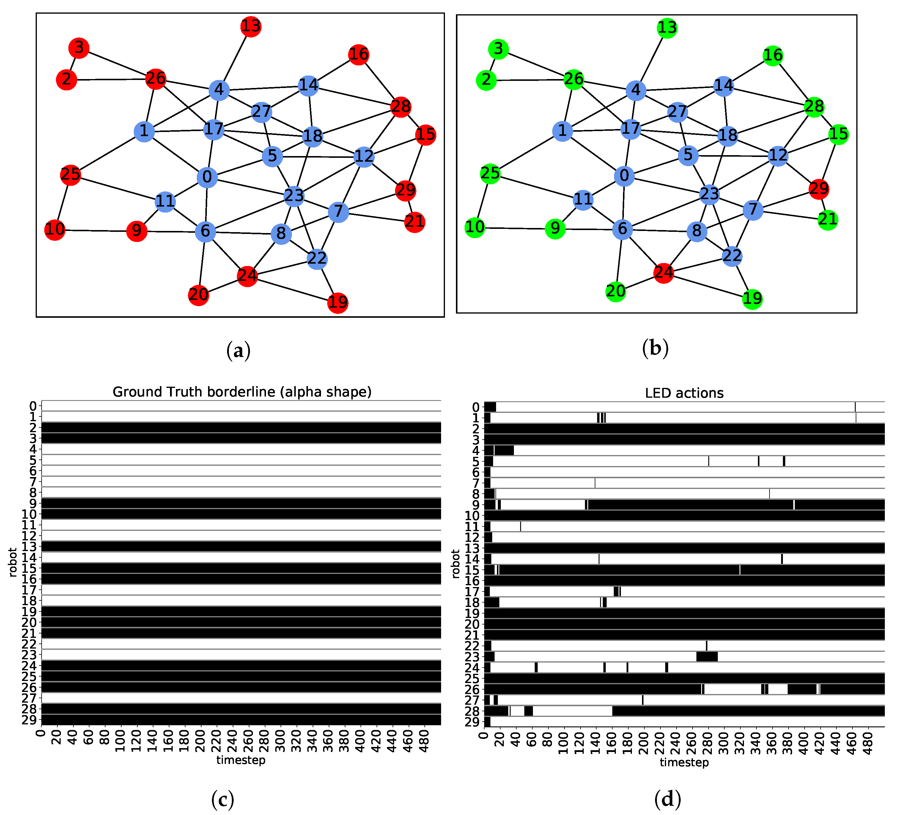
Behavior: In order to assess the correct functioning of the evolved solution, Figure 10 shows the behavior of the robots in a trial with 30 agents. Firstly, Figure 10a, illustrates the swarm spatial distribution and pairwise communication channels. Red balls represent robots belonging to the alpha shape with $\alpha =15$ (see Section 4) and blue dots represent interior nodes. For the depicted graph, Figure 10c exposes the target LED actions or target alpha shape that the robots should perform in order to correctly identify the swarm borderline. Thus, the robots with horizontal black bars are members of the borderline according to the alpha shape algorithm. Additionally, Figure 10d shows the actual LED actions of the robots, indicating if they are in the frontier or in the interior. Figure 10b displays, in the spatial swarm distribution, the correct frontier classifications (in green) and the errors (in red). The actions of Figure 10b correspond to a snapshot at time instant 480. Observing Figure 10d, the results show outstanding classification accuracy, although sporadically there are some robots whose decision is incorrect (excluding the first 10 time steps, the classification accuracy oscillates between 83%, for instants near time step 80, and 93%, for the last cycles of the trial). Specifically, there are about 2 or 3 robots, depending on the observed time step, whose classification is wrong. It can be observed that there are some agents whose LED actions are remarkably stable (e.g., robots 2, 3 or 10) while the decisions of other robots are much more undefined (e.g., nodes 9, 26 or 28). A common observable feature is that agents with a robust decision generally have only few neighbors (1 or 2). On the contrary, unstable robots mainly belong to a dense part of the graph, with many neighbors (3, 4 or 5). Thereafter, the errors principally occur when the agents have many neighboring robots, leading to the naive classification of being interior node (which is an incorrect assumption in some cases).

Furthermore, another interesting observation is that errors are more likely to appear as false negatives as it can be observed in Figure 11, where the true positive rate (TPR) is slightly inferior than the true negative rate (TNR). At the initial time steps of the simulation, the TPR and the TNR are respectively 1 and 0 because, at the simulation startup, all the agents identify themselves as frontier nodes (see Figure 10d).

To observe the behavior in a more visual manner, Figure 12 collects snapshots of a sample trial at different time instants of the simulation. At the initial time step, all robots consider themselves as extremities (red balls). Subsequently, as time elapses, the solution is corrected until the final decision is settled (approximately at time instant 50). The actual alpha shape of the example is shown in purple in Figure 12f. The final classification of this example results in two errors, corresponding to false negatives in both cases. Finally, the behavior of the solution to this experiment can be observed in video format (https://youtu.be/tGytXx2BM2w accessed on 22 Janunary 2021).

Scalability: In Figure 13, the scalability of the system is evaluated. The results are presented using a sample of size 50 with independent simulation executions. For each swarm size, it shows the accuracy of each time step, defined as the number of agents correctly identified as frontier or interior divided by the swarm size. The curves represent the time dependent median of the accuracy using all the collected samples. Alternatively, the shadow areas indicate, at each time instant, the first and third quantiles of the accuracies. It can be observed that the solution scales utterly well as swarm size increases. Indeed, there is no statistically significant degradation in accuracy as the number of robots grows, up to 50 agents. Consequently, the scalability of the system is clearly fulfilled.

Robustness: The robustness capabilities are evaluated by reinitializing the robots spatial graph, defining their positions, every 200 time steps. However, the states of the CTRNNs of all the robots are maintained untouched regardless of the position resampling. This causes an abrupt change in the swarm topology, leading to agents being forced to reconsider if they are in the borderline subset. Figure 14 displays both target borderline temporal evolution (left) and robots LED actions (right). Although there are several erroneous decisions, robots are generally able to respond successfully to topological alterations.

Figure 15 represents the accuracy distributions for different swarm sizes under the above mentioned topology alterations. Evidently, there is a short transient period of time required by the agents to notice the swarm changes and alter its neural states as a consequence. The resampling of robot positions result in discontinuous accuracy drop as the alpha shape and, thus, the robots in the borderline, change. Agents are able to detect the changes and almost correctly solve the task for the unexpected swarm redistribution.

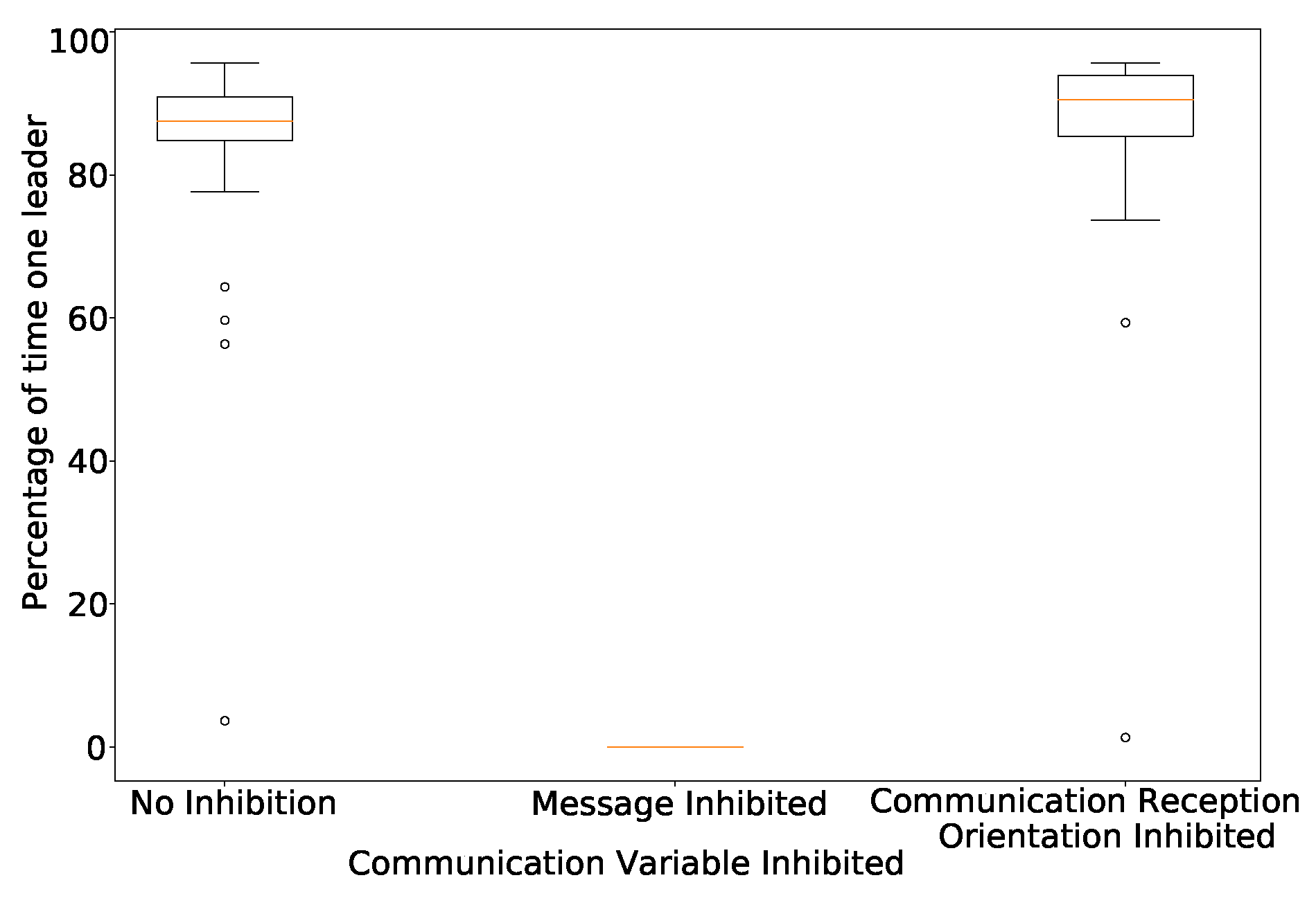
Communication: With the aim of studying the communication that emerges as a result of evolution, Figure 16 analyzes the importance of the communication variables in solving the task. Specifically, in the figure, it can be observed the accuracy comparison among a scenario with no inhibition and when different communication variables are inhibited. Each inhibition is performed one by one and consists in replacing the value of the corresponding variable with zeros at the input of the CTRNN. The comparison of the figure reveals that the information about the orientation from where the message was sensed is a highly relevant context variable, whose deletion causes system breakdown. On the contrary, provided that the system accuracy is not significantly decreased, the results indicate that the message is not harnessed in this experiment. This leads to a solution to the task with purely situated communication, in which only the context underlying the message carries information. The communication state was not included because we observed that the CTRNN of the robots always settle the state to send mode. In relation to the message reception orientation, it is remarkably challenging to find out the precise functioning and usage of its information.

6. Conclusions

A set of robotics tasks were proposed and solved using a swarm of homogeneous simulated robots, controlled by Continuous-Time Recurrent Neural Networks (CTRNN). The neural controllers are optimized using Separable Natural Evolution Strategies (SNES). The faced experiments were the leader selection and the swarm borderline identification tasks. These experiments required, at some extent, the cooperative interaction and communication among robots, that are incapable of solving the problem individually. The objective of the leader selection experiment is to elect, automatically and in a distributed fashion, a single leader of the swarm of robots. Alternatively, the borderline identification is a task in which swarm members have to detect if they are in the borderline or shape of the swarm or not. In both experiments, the simulated static robots have to solve the corresponding task in a distributed manner by interacting locally using a communication system. The semantics of the communication are undefined a priori and it corresponds to the evolution process and fine-tuning of the neural controller the settlement of the communication information that becomes relevant. As a side contribution of this paper, we propose a minimal communication system, highly constrained both in terms of spatial range and number of messages that can be received at each time instant. It provides the robots with both a message and the context information attached to it. We analyzed the emerged communication mechanics of both tasks that result from evolution. The main objective and contribution of this paper is the validation of the hypothesis that, depending on the task to be solved, the evolution guides communication towards very different mechanics and semantics, albeit the neural controller is architecturally the same. We show that evolution in the leader selection experiment leads to an abstract communication, while in the borderline identification task only the environmental context is used. Specifically, the abstract communication that emerged in the former experiment was a signaling process in which leaders notify their leadership and non leaders relay the information so that it is spread around the entire swarm. On the contrary, a purely situated communication, in which only the context information about the orientation from where the message was received seems to be relevant, arises in the latter experiment.

Finally, we show that, up to considerable limits, the evolved systems are scalable and outstandingly robust under the defined perturbations. After the evolution phase, the scalability of both experiments was assessed by means of increasing the swarm size and observing the consequent results. Additionally, the robustness of the leader selection task was evaluated by imposing leader fault after 50 consecutive time steps of stable leadership. In the borderline identification experiment, the system robustness was verified by drastically altering the swarm topology at runtime.

Although the expected results were successfully achieved, there are some limitations that should be taken into consideration and can be stated as future research lines. Firstly, owing to the fact that the experiments are carried out using simulated robots, a future analysis employing real robots must be accomplished in order to address the simulation-to-reality gap. Moreover, the experiments are performed using a swarm of static robots. Thus, it has not been assessed if the system is able to respond suitably in dynamic environments. Additionally, we show that the same neural controller can be optimized to reach the emergence of diverse communication semantics depending on the task to be solved. However, this validation is only assessed for the leader selection and borderline identification problems. Therefore, a future study can extend this work to more demanding and sophisticated tasks that require a more complex and higher level communication semantics.

The future lines of research that have appeared during the development of this paper are the following. Firstly, in order to extend the findings of this paper, an important future improvement of this work would be to adapt the neural controller to more diverse and potentially more complex swarm robotics tasks (e.g., experiments involving robot locomotion by adding differential drive system control actions at the neural level). Therefore, it can be further assessed if more complex communication semantics, apart from those encountered in this study, can emerge using the same controller. Secondly, a more ambitious experiment would be to verify if it is possible to evolve a robot’s neural controller capable of solving multiple problems (multitasking), either sequentially or concurrently. Consequently, it could be analyzed if the multitasking capability also leads to the emergence of multiple coexisting communication semantics. Additionally, an exhaustive analysis of the optimal value of $\delta$ (see Section 3.2) for the experiments would require a demanding research labor and weeks of optimization and simulations. Therefore, a remarkably interesting future research line is the analysis of the impact of the value of $\delta$ on the emergence of communication. Furthermore, because the experiments are carried out using simulated robots, a future analysis employing real robots must be accomplished in order to address the simulation-to-reality gap. Finally, the experiments are performed using a swarm of static robots. Thus, it has not been assessed if the system is able to respond suitably in dynamic environments. This extension, jointly with the addition of more complex and elaborated experiments, is also a future improvement to be considered.