Control of a Robotic Swarm Formation to Track a Dynamic Target with Communication Constraints: Analysis and Simulation

Abstract

We describe and analyze the Local Charged Particle Swarm Optimization (LCPSO) algorithm, that we designed to solve the problem of tracking a moving target releasing scalar information in a constrained environment using a swarm of agents. This method is inspired by flocking algorithms and the Particle Swarm Optimization (PSO) algorithm for function optimization. Four parameters drive LCPSO—the number of agents; the inertia weight; the attraction/repulsion weight; and the inter-agent distance. Using APF (Artificial Potential Field), we provide a mathematical analysis of the LCPSO algorithm under some simplifying assumptions. First, the swarm will aggregate and attain a stable formation, whatever the initial conditions. Second, the swarm moves thanks to an attractor in the swarm, which serves as a guide for the other agents to head for the target. By focusing on a simple application of target tracking with communication constraints, we then remove those assumptions one by one. We show the algorithm is resilient to constraints on the communication range and the behavior of the target. Results on simulation confirm our theoretical analysis. This provides useful guidelines to understand and control the LCPSO algorithm as a function of swarm characteristics as well as the nature of the target.

1. Introduction

Controlling the collective behavior of a large number of robots is a complex task. However, large natural multi-agent systems are known to work very well, such as bird flocks [1,2,3], fish schools [2,4,5], ants using pheromones [2,6], or aggregations of bacteria [2,7,8]. These self-organized systems have served as a source of inspiration to control large formations of robots to prevent collisions between these robots [9]. The emergence principle where complex collective behaviors arise from simple, elementary rules governing individuals is the main topic of interest for artificial swarming systems. However, the emergence of swarm behavior requires some constraints on the number of agents, the environment, and so forth. Also, it is difficult to design the elementary rules for a specific desired collective behavior to emerge.

One behavior in particular, flocking or schooling, enjoys a growing interest in the scientific domain. Ref. [10] established a first landmark, giving the three rules of flocking (alignment, cohesion, separation). Then Tanner, Jadbabaie and Pappas, in a two-part article [11,12], made a fundamental mathematical analysis of the Reynolds rules using the Artificial Potential Field (APF) approach. They proved that using potentials both attractive and repulsive, the flock becomes homogeneous with equal inter-agent distance and equal speed vectors at equilibrium. This behavior is resilient to external stimuli as long as the agents are within communication range. By using these methods, and despite the remaining challenges to designing the desired group behavior, the robotics community has used swarm-based approaches for applications such as target tracking [13,14,15,16,17], Search And Rescue (SAR) [18], or Odor Source Localization (OSL) [19,20,21,22,23,24,25,26], among others.

Ant Colony Optimization (ACO) [6] or Particle Swarm Optimization (PSO) [27] are swarm intelligence algorithms used in the mathematical community of optimization. The strength of these approaches lies in using agents distributed in the workspace, sharing information to search for the optimum of a fitness function. In particular, this community strongly uses the PSO algorithm [13,14,15,18,19,20,21,28]. It is important to stress that optimization algorithms like PSO, can also drive a swarm of actual robots [29]. This bridge between the two communities of robotics and optimization shows that one common way to solve their respective problems can be found through swarming.

In the present paper, we focus on tracking a mobile target leaving a semi-permanent trail, such as a chemical scent or radioactive particles carried by the environment. This problem could be described as Mobile Odor Source Localization (MOSL), a generalization of OSL. We assume the information to be “scalar”, in that its value is a real, one-dimensional number. As Section 2 will show, this problem is equivalent to maximizing a fitness function varying with space and time. The plume model is simplified compared to the state-of-the-art [30,31] to fasten the simulation results and obtain preliminary results but those models will be upgraded in a future work. In a terrestrial environment, instances of this problem arise for example, when tracking a moving source of nuclear radiation with possible counter-terrorist applications [32,33], or finding the origin of polluted areas [34]. Applications in the marine field include securing a specified area to detect intruders; to prevent illegal oil discharges by ships using so-called “magic pipes”; localizing a pipeline leak [35,36], or various other similar uses. A variant of PSO called Charged Particle Swarm Optimization (CPSO) was proposed by [20,21] to solve OSL and head for a static odor source, with interesting results [37]. CPSO differs from PSO in that repulsive components are added to avoid collisions between agents in the swarm. The equations of flocking correlate with CPSO [38,39], or more recently with the Extended PSO [28], but no mathematical analysis has yet linked up those two fields.

In [40], for our MOSL problem, we proposed an algorithm called LCPSO, inspired by CPSO, which takes into account communication constraints in distance between agents that are representative of underwater systems [41]. Based on simulations, we showed that the limited number of attracting agents allows a reactive tracking of one or multiple moving targets avoiding collisions between agents, with better performances than the CPSO algorithm. In this paper, we intend to demonstrate new results characterizing LCPSO. First, we demonstrate that the positions of the center of gravity and attractor(s) will guide the swarm, and this mechanism is the key to head for the source. Second, we show that a distance parameter, $r_{eq}$, which is an input of our algorithm, can control the surface of the swarm. Finally, we show that, whatever the initial conditions, the swarm will attain a stable formation, invariant to time and the place of the attractor. We prove these results theoretically under some simplifying hypotheses, whatever the dimension D. We then successively remove the simplifying hypotheses and show that the proposed theoretical results are confirmed by simulations. These flocking behaviors have already been shown in [12,39]. However, to the best of our knowledge, controlling the surface of the swarm with an optimization algorithm such as PSO and its derivatives is new. Also, the use of specific attractors to head for a goal indirectly and in the same time keeping a strong formation, has never been investigated before, to the best of our knowledge.

We organize our article as follows. Section 2 formalizes the MOSL problem while Section 3 describes our models, particularly the PSO algorithm and the LCPSO algorithm to track a mobile target. New contributions begin at Section 4, which provides a mathematical analysis of the behavior of the LCPSO algorithm under some restricting hypotheses. Those hypotheses are removed one by one to show that our algorithm is resilient to a limited communication range. Section 5 provides simulations results of our algorithm in mobile target tracking scenario. Finally, Section 6 concludes this paper and gives some perspectives for future works.

2. Problem Formulation

2.1. The General MOSL Problem

We extend the OSL problem, where the odor source is static, to the case of moving source resulting in the MOSL problem. The objective is to localize a mobile target, characterized by a D-dimensional position ${\mathbf{p}}_s\left(t\right)$ varying with time t. This target is assumed to release scalar information in the environment, such as an odor, heat, radioactivity, a sound or radio wave; without losing generality we assume the intensity of this information to be positive. We thus note $u:{\mathbb{R}}^D\times \mathbb{R}\mapsto {\mathbb{R}}^{+};(\mathbf{p},t)\to u\left(\mathbf{p},t\right)$. This information u is assumed to be diffused and transported by the environment. This can be modeled by a partial differential equation of variable u, which exact formulation depends on the problem at hand. We assume furthermore that at any given time t, function u has an unique point ${\mathbf{p}}_{\max }\left(t\right)$ where the information intensity u is maximum. We also assume that the diffusion and transport mechanism is such that ${\mathbf{p}}_{\max }\left(t\right)$ is very close to the position of the target ${\mathbf{p}}_s\left(t\right)$ so that for all practical purposes we may assume that ${\mathbf{p}}_s\left(t\right)\approx {\mathbf{p}}_{\max }\left(t\right)$, that is, both terms can be used interchangeably. Our problem is then to find ${\mathbf{p}}_{\max }\left(t\right)$, which is then equivalent to finding the position of the target at the same date. Another thematic close to MOSL is geofencing [42] where Unmanned Aerial Vehicles (UAV) can be used in a constrained area, typically cities, for tracking and tracing missions, as for the track of stolen cars.

The measure, made by the system’s sensors, will be denoted by function $f:{\mathbb{R}}^D\times \mathbb{R}\mapsto {\mathbb{R}}^{+};(\mathbf{p},t)\to u\left(\mathbf{p},t)+\beta (\mathbf{p},t\right)$, where $\beta (\mathbf{p},t)$ is a noise. We assume that the Signal-to-noise Ratio (SNR) is sufficient so that the maximum of f still coincides with the maximum of u for all practical purposes. In our simulations, we considered that function u had values in $[0,1]$ and the noise was additive white Gaussian, uncorrelated in space and time, with a standard deviation $\sigma$ taken between 0 and $0.25$ except where indicated. We leave issues raised by a poor SNR for future research.

2.2. The Toy Problem Used in This Paper

Instead of describing the problem by a partial derivative equation, we may instead assume that the solution of this equation is known explicitly. This is the approach we use in the simulations presented in this paper because this is quicker to simulate. We use for instance the following expression:

$$\left\{\begin{array}{c}u(\mathbf{p},t+\Delta t)=\underset{1}{\underbrace{\frac{1}{1+{∥\mathbf{p}-{\mathbf{p}}_s\left(t\right)∥}^2}}}+\underset{2}{\underbrace{(1-e^{-\frac{\Delta t}{\tau }})u(\mathbf{p},t)}}\hfill \\ f(\mathbf{p},t)=u(\mathbf{p},t)+\underset{3}{\underbrace{\beta (\mathbf{p},t)}}.\hfill \end{array}\right.$$

(1)

In these equations, $\Delta t$ is a discrete time step. The Equation (1) contains three elements to represent real-world phenomena:

(1)

a spatial term which decreases with the distance between target position ${\mathbf{p}}_s$ and any position $\mathbf{p}$ in the workspace; this is the inverse square law induced by mechanisms of conservation of power through propagation, modified with a constant additive term in the denominator to prevent the value from becoming unreasonably large when $∥\mathbf{p}-{\mathbf{p}}_s\left(t\right)∥\to 0$;

(2)

a temporal term, representing a decay, inspired by the response to a first-order filter model parameterized by the time constant $\tau$;

(3)

an additive white Gaussian noise $\beta (\mathbf{p},t)\sim \mathcal{N}(0,\sigma )$ in the whole environment, with $\sigma \ll$ max$\left(f\right)$, representing measurement noise.

In our paper, dimension D can be 1 or 2 or more, and it will be indicated explicitly when it is necessary. Simulation results are not treated in higher dimensions, but we assume that the results we present should be close to the results displayed in Dimension 2 because there are no cross-dimensional terms in the PSO equation described below in Expression (2).

We must stress that the exact mechanism behind the generation of function u does not need to be known for the problem to be solved. The only hypotheses that matter, are that (i) there is only one spatial maximum for u at each date and (ii) that the maximum is reached close to the actual position of the target at a given date. This way, all that matters is finding the maximum of u at each date by sampling f at the positions of the agents in the swarm.

This model is less complex that in the state-of-the-art [31,37,43], where the plume model is dynamic and with multiple local maxima. Environmental sensors help the modelisation of this plume, an anemometer or ocean current sensor for example. However, in OSL, the source is static, and the important point we wanted to highlight is the unpredictability of the source behavior. Hence, study our algorithm with both the plume and source dynamics will complicate the analysis of our algorithm. For this reason, the analysis takes into account only the dynamics of the source, and an analysis with a dynamic plume model will be part of a future work. We note that the measurement noise can create multiple local maxima, but this phenomenon can disappear instantaneously at the next time step for the agent i.

3. Models

3.1. The PSO Algorithm

PSO is an evolutionary algorithm, inspired by flocking birds [27]. We consider N trackers sampling f at their position ${\mathbf{p}}_i\left(t\right)$. This value is given by $f\left({\mathbf{p}}_i\left(t\right),t\right)$ from (1). The trackers move to maximise $f({\mathbf{p}}_i\left(t\right),t)$. To do this, the PSO algorithm provides an update of the speed vector ${\mathbf{v}}_i\left(t\right)$ as follows:

$$\begin{array}{cc}\hfill {\mathbf{v}}_i(t+\Delta t)=& \underset{1}{\underbrace{c_0{\mathbf{v}}_i\left(t\right)}}+\underset{2}{\underbrace{c_1{\alpha }_{i1}\left(t\right)\left({\mathbf{p}}_i^b\left(t\right)-{\mathbf{p}}_i\left(t\right)\right)}}+\underset{3}{\underbrace{c_2{\alpha }_{i2}\left(t\right)\left({\mathbf{p}}^g\left(t\right)-{\mathbf{p}}_i\left(t\right)\right)}}.\hfill \end{array}$$

(2)

As described in (2), the speed vector at time $t+\Delta t$ is a sum of three elements:

(1)

The previous speed vector of tracker ${\mathbf{v}}_i\left(t\right)$, weighted by a constant coefficient $c_0$. For the convergence of the algorithm, we need to have $c_0\in ]-1;1[$ [44]. $c_0$ is homogeneous to a (pseudo) mass and is sometimes called “inertia” in the community.

(2)

The difference between the current position of tracker i and its best historical position noted ${\mathbf{p}}_i^b\left(t\right)$ ( “b” for “$best$”). The best historical position ${\mathbf{p}}_i^b\left(t\right)$ is the position ${\mathbf{p}}_i\left(t_i\right)$, with $t_i$ between time 0 and t where measure $f({\mathbf{p}}_i,t_i)$ was the greatest. This component is weighted by a constant coefficient $c_1$.

(3)

The difference between the position ${\mathbf{p}}^g\left(t\right)$ (“g” for “$global$”) of the current swarm’s best tracker and the current position of tracker i. The position of the best tracker of swarm ${\mathbf{p}}^g\left(t\right)$ is the tracker j measuring the greatest $f({\mathbf{p}}_j,t)$ among the N trackers of the swarm. This component is weighted by a constant coefficient $c_2$.

The second and last components are attractors, weighted by a random number, respectively ${\alpha }_{i1}\left(t\right)$ and ${\alpha }_{i2}\left(t\right)$, uniformly distributed in $[0,1]$ and specific to agent i. These random numbers provide diversity to the system and improve exploration, avoiding the swarm to be trapped in a local optimum [27,45].

Using the Euler integration scheme, the updated position of tracker i is computed as the sum of its previous position and the updated speed vector as follows [27]:

$${\mathbf{p}}_i(t+\Delta t)={\mathbf{p}}_i\left(t\right)+\Delta t·{\mathbf{v}}_i(t+\Delta t).$$

(3)

3.2. APF Theory and Flocking Principles

In APF methods, the analysis is based on potential functions $P\left(d_{i,j}\left(t\right)\right)$, where $d_{i,j}\left(t\right)=∥{\mathbf{p}}_i\left(t\right)-{\mathbf{p}}_j\left(t\right)∥$ is the Euclidean distance between agents i and j. The agent i uses a gradient descent algorithm based on $P\left(d_{i,j}\left(t\right)\right)$ to move. In flocking algorithms, we are interested in a particular potential function $P\left(d_{i,j}\left(t\right)\right)$, described in Definition 1.

Definition 1.

The potential function $P\left(d_{i,j}\left(t\right)\right)=P^a\left(d_{i,j}\left(t\right)\right)-P^r\left(d_{i,j}\left(t\right)\right)$ is a flocking potential field if:

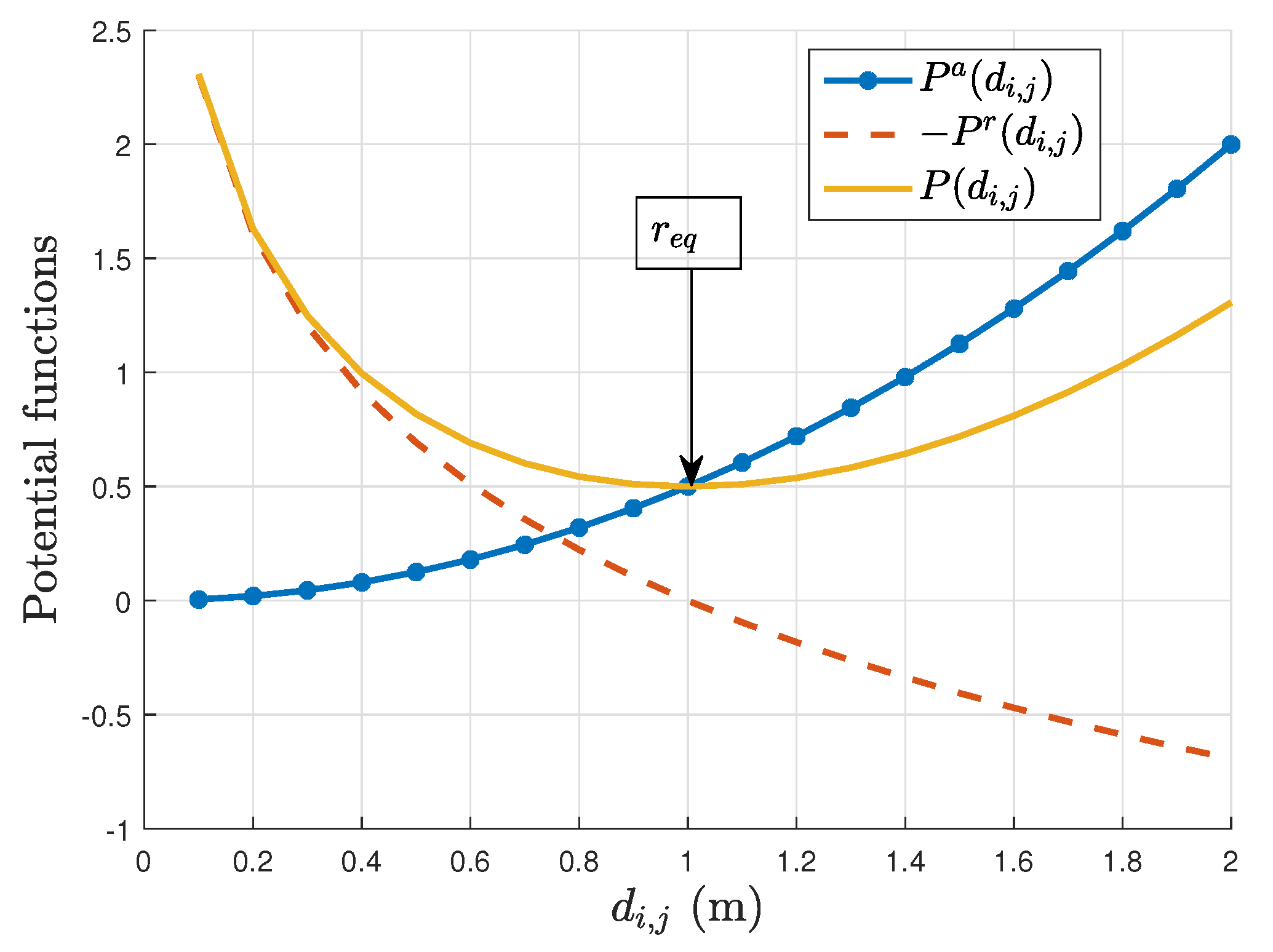
• $P\left(d_{i,j}\left(t\right)\right)$ is a non-negative function of the distance $d_{i,j}\left(t\right)$ between agents i and j,
• $P^r\left(d_{i,j}\left(t\right)\right)$ is monotonically increasing in $[0,+\infty [$ and its gradient is the highest when $d_{i,j}\left(t\right)\to 0$,
• $P^a\left(d_{i,j}\left(t\right)\right)$ is monotonically increasing in $]0,+\infty [$ and its gradient is the highest when $d_{i,j}\left(t\right)\to +\infty$,
• $P\left(d_{i,j}\left(t\right)\right)$ is convex and even,
• $P\left(d_{i,j}\left(t\right)\right)$ attains its unique minimum when i and j are located at a desired distance $r_{eq}$.

Where $P^a\left(d_{i,j}\left(t\right)\right)$ and $P^r\left(d_{i,j}\left(t\right)\right)$ are, respectively, attractive and repulsive potential fields. An example of such potential fields are shown in Figure 1. It is a reactive approach to guidance where the trajectory is not planned. Since $P\left(d_{i,j}\left(t\right)\right)$ is convex, we can directly use the sign of its gradient to describe the behavior of agents i and j. If the gradient is positive, then agents i and j will repel each other. If the gradient is negative, then agents i and j will attract each other. The agent will stop when it attains an equilibrium distance $r_{eq}$ between agents i and j, where the potential function is null and stable in the sense of Lyapunov [12,35,38]. Collisions between neighbors in the swarm are thus avoided and the inter-agent distance is controlled owing to near-equilibrium distance parameter $r_{eq}$. Hence, the swarm will attain a stable formation, when individually each agent minimizes its potential function, whatever the initial position of the agents. When the swarm is stable, there is a velocity matching between the agents [12,46]. Ref. [47] use the consensus metric $V\left(t\right)$ as follows:

$$V\left(t\right)=\frac{{\sum }_{i=1}^N{\sum }_{j=1,j\ne 1}^N∥{\mathbf{v}}_i\left(t\right)-{\mathbf{v}}_j\left(t\right)∥}{N(N-1)}.$$

(4)

Hence, if ${lim}_{t\to +\infty }V\left(t\right)=0$, we are sure to attain a consensus in the swarm speed. We define as follows the swarm stability.

Definition 2.

The swarm is stable if there is a consensus as follows:

$$\forall ϵ>0,\exists t_0/\forall t\ge t_0,V\left(t\right)<ϵ.$$

3.3. PSO Formulated Using the APF Theory

As we have introduced APF theory and flocking principles, we can now rewrite the PSO Equation (2) as a gradient descent strategy:

$${\mathbf{v}}_i(t+\Delta t)=c_0{\mathbf{v}}_i\left(t\right)-{\nabla }_{{\mathbf{p}}_i}{P}_i\left(t\right).$$

(5)

Here, $P_i\left(t\right)$ is the potential field of PSO applied to agent i, providing equality of Equations (2) and (5). Since potential fields use only phenomena of attraction/repulsion with inter-agent distance, weight $c_0$ does not appear in potential field $P_i\left(t\right)$. So we find:

$$\begin{array}{cc}\hfill P_i\left(t\right)& =P^a\left(∥{\mathbf{p}}_i^b\left(t\right)-{\mathbf{p}}_i\left(t\right)∥\right)+P^a\left(∥{\mathbf{p}}^g\left(t\right)-{\mathbf{p}}_i\left(t\right)∥\right)\hfill \\ \hfill & =\frac{c_1{\alpha }_{i1}\left(t\right)}{2}{∥{\mathbf{p}}_i^b\left(t\right)-{\mathbf{p}}_i\left(t\right)∥}^2+\frac{c_2{\alpha }_{i2}\left(t\right)}{2}{∥{\mathbf{p}}^g\left(t\right)-{\mathbf{p}}_i\left(t\right)∥}^2.\hfill \end{array}$$

(6)

Here, $P^a\left(d_{i,j}\left(t\right)\right)$ is a generic potential attraction field known in APF literature as a quadratic attractor [48]:

$$P^a\left(d_{i,j}\left(t\right)\right)=A·d_{i,j}^2\left(t\right),$$

(7)

where A is a random number uniformly distributed in $[0,\frac{c_1}{2}]$ and $[0,\frac{c_2}{2}]$ respectively. Hence, when the algorithm converges, all the agents will be located at the same position. So, to apply this algorithm to robotics, we need to include repulsive mechanisms to be coherent with Definition 1.

3.4. The LCPSO Algorithm

3.4.1. Adding an Anti-Collision Behavior to PSO: CPSO

The objective here is to determine a potential field $P_i\left(t\right)$, inspired by PSO potential (6), that meets Definition 1. To do this, Ref. [20] introduced a variation of PSO, called CPSO, which was demonstrated experimentally with interesting results [20,37]. To derive the equations of CPSO, we define the following unbounded repulsive potential [39]:

$$P^r\left(d_{i,j}\left(t\right)\right)=log\left(d_{i,j}\left(t\right)\right).$$

(8)

This potential verifies that $P^r\left(d_{i,j}\left(t\right)\right)\to -\infty$ when $d_{i,j}\left(t\right)\to 0$. If we sum the attractive potential (7) and the repulsive one (8), we obtain a potential that meets Definition 1.

Those models of potentials are not unique. The state of the art provides good examples of possible potential functions for flocking algorithms [38,39]. However, for the analysis at equilibrium, we need the attractive potential defined in (7) for two reasons. First, we keep the links with the original PSO algorithm. Second, this particular model is necessary for some theorems, Theorem 4 in particular, which is important to determine the characteristics of our swarm formation.

The repulsive potential is then added to the PSO equation:

$$\begin{array}{cc}\hfill {\mathbf{v}}_i(t+\Delta t)=& c_0{\mathbf{v}}_i\left(t\right)+c_1{\alpha }_{i1}\left(t\right)\left({\mathbf{p}}_i^b\left(t\right)-{\mathbf{p}}_i\left(t\right)\right)\hfill \\ \hfill & +c_2{\alpha }_{i2}\left(t\right)\left({\mathbf{p}}^g\left(t\right)-{\mathbf{p}}_i\left(t\right)\right)-c_3\sum _{j=1,j\ne i}^N{\nabla }_{{\mathbf{p}}_i}{P}^r\left(d_{i,j}\left(t\right)\right),\hfill \end{array}$$

(9)

where $c_3$ is the constant repulsive weight between trackers i and j.

3.4.2. LCPSO, a CPSO Variant to Deal with Some Real-World Constraints

First, to reflect limitations in communication links, a local communication constraint is added to the model. Indeed, the best tracker position of the swarm ${\mathbf{p}}^g\left(t\right)$ in Equation (9) is global, shared with each agent of the swarm. We use the local-best vector position ${\mathbf{p}}_i^l\left(t\right)$ (l for local), which is the position of tracker j in the neighborhood set of i where measure $f({\mathbf{p}}_j,t)$ is the greatest. The neighborhood set ${\mathcal{N}}_i\left(t\right)$ is based on parameter $r_{com}$ which denotes the maximum communication range between tracker i and its neighbors [12]. Beyond maximum communication range $r_{com}$ data transmission is impossible, below $r_{com}$ transmission is perfect:

$${\mathcal{N}}_i\left(t\right)=\left\{j\right|∥{\mathbf{p}}_i\left(t\right)-{\mathbf{p}}_j\left(t\right)∥<r_{com},i\ne j\}\subset \{1,\cdots ,N\}.$$

(10)

This decentralization was already proposed by [14,15] but to the best of our knowledge it was never used in the aim of mobile target tracking. Each vehicle will have its own local best position and will move towards its best neighbor.

Second, the best historical position ${\mathbf{p}}_i^b\left(t\right)$ is removed in the proposed approach. This is because the target is not static: it changes position with time.

Finally, to obtain a stable swarm formation, we set our random component ${\alpha }_{i2}\left(t\right)$ to 1. The analysis of the algorithm with random components can be the object of future work. Those considerations lead to the following model, originally introduced in [40], and which we named LCPSO:

$$\begin{array}{cc}\hfill {\mathbf{v}}_i(t+\Delta t)=& c_0{\mathbf{v}}_i\left(t\right)+c_2\left({\mathbf{p}}_i^l\left(t\right)-{\mathbf{p}}_i\left(t\right)\right)-c_3\sum _{j\in {\mathcal{N}}_i\left(t\right)}{\nabla }_{{\mathbf{p}}_i}{P}^r\left(d_{i,j}\left(t\right)\right).\hfill \end{array}$$

(11)

From Equation (11), we can deduce the potential function of LCPSO as follows:

$$P_i\left(t\right)=P^a\left(∥{\mathbf{p}}_i^l\left(t\right)-{\mathbf{p}}_i\left(t\right)∥\right)-\sum _{j\in {\mathcal{N}}_i\left(t\right)}{P}^r\left(d_{i,j}\left(t\right)\right)$$

(12)

This potential meets Definition 1, and is illustrated in Figure 1, with the corresponding attractive (7) and repulsive potentials (8) used for the LCPSO. The Euler integration scheme is the same as in Equation (3).

4. Analysis of the Properties of LCPSO

4.1. Metrics and Hypothesis

While we already illustrated the behavior of the LCPSO algorithm earlier through simulation [40], these properties were only shown intuitively. We now wish to give some mathematical basis to this intuition. We make the following assumptions that will be valid throughout the mathematical analysis of this section:

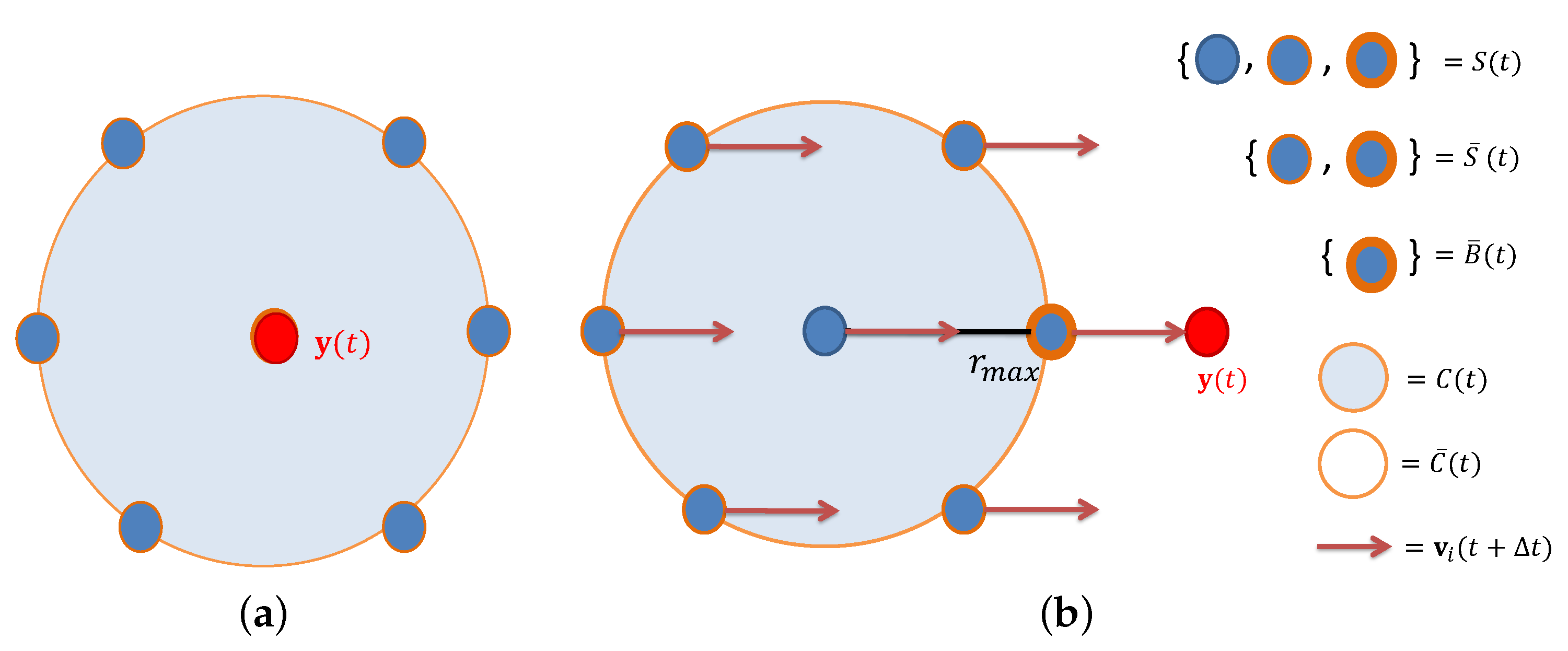
• Communication range is unlimited. As a result, the local-best attractor ${\mathbf{p}}_i^l\left(t\right)$ is the best tracker position of the swarm ${\mathbf{p}}^g\left(t\right)$.
• We focus our efforts on the APF analysis, and to ease the analysis we set $c_0$ to 0. So the speed vector ${\mathbf{v}}_i(t+\Delta t)$ is updated only with the gradient descent of the potential field equation.
• The target’s behavior is not known from the swarm’s point of view and can be dynamic. Tracker i measures $f({\mathbf{p}}_i,t)$ and adjusts its local-best position ${\mathbf{p}}_i^l\left(t\right)$ as a function of maximum measurement of the neighborhood. Since the communication range is small, we make the hypothesis that information exchange is instantaneous between the trackers and is limited to their position in absolute coordinates and their measurements, without noise.

To illustrate the inter-agent distance between nearest neighbors in the swarm, we introduce a new function, the swarm spacing $\rho \left(N\right)$. We normalize this spacing by $r_{eq}$, a parameter allowing us to control the inter-agent equilibrium distance when the swarm is stable, and the number of agents N:

$$\rho \left(N\right)=\frac{1}{r_{eq}·N}\sum _{i=1}^N\underset{i\ne j}{min}{d}_{i,j}.$$

(13)

Another important parameter is the surface area taken up by the swarm. For some cases, this parameter is critical to have a good tracking of the source. As we will see in Section 4.2, swarm formations have a convex hull inside a ball, and we will thus be able to represent this surface with only one parameter, the radius of this ball $r_{max}$. Whatever the dimension, we have:

$$r_{max}=\underset{i\in [1,\cdots ,N]}{max}\frac{∥\overline{\mathbf{p}}-{\mathbf{p}}_i∥}{r_{eq}}.$$

(14)

With $\overline{\mathbf{p}}$ the center of gravity of our swarm, represented by the following equation:

$$\overline{\mathbf{p}}\left(t\right)=\frac{1}{N}\sum _{i=1}^N{\mathbf{p}}_i\left(t\right).$$

(15)

Our swarm model has a lot of mathematical similarities with the models of [39]. So, for conciseness, the demonstrations too close from [39] are not given, and the other ones are in the Appendix A. Moreover, all the theorems presented in this paper are true regardless of the repulsive potential $P^r\left(d_{i,j}\right)$, as long as it respects Definition 1. Thus, we could imagine that, if the repellent potential is not suitable, we could test others that exist in the state of the art [38,39].

4.2. Behavior of LCPSO

We suppose that the agents’ positions are taken in ${\mathbb{R}}^D$, with D the dimension. $S\left(t\right)$ is the set of agents’ positions ${\mathbf{p}}_i\left(t\right)$ of the swarm at time t, $i\in [1,\cdots ,N]$. Let us note $C\left(t\right)$ as a convex hull of $S\left(t\right)$: it is a continuous subset of ${\mathbb{R}}^D$. Then let us note $\overline{C}\left(t\right)$ as the convex polygon of $S\left(t\right)$. It is a manifold of dimension $D-1$ which displays the surface taken by the swarm. We set $\mathbf{y}\left(t\right)\in {\mathbb{R}}^D$ the optimum position of f at date t: $\mathbf{y}\left(t\right)={arg\; max}_{\mathbf{y}}f(\mathbf{y},t)$. We suppose that this optimum is unique and is the position of the target ${\mathbf{p}}_s\left(t\right)$ propagating information.

We define the set $B\left(t\right)$, which contains the best attractors of the swarm at time t which minimised the Euclidean distance with respect to $\mathbf{y}\left(t\right)$.

$$B\left(t\right)=\{\mathbf{p}\left(t\right)\in {\mathbb{R}}^D|\mathbf{p}\left(t\right)=\underset{\mathbf{p}\left(t\right)\in S\left(t\right)}{arg\; min}∥\mathbf{p}\left(t\right)-\mathbf{y}\left(t\right)∥\}.$$

(16)

The set $S\left(t\right)$ being discrete, we introduce the set $\overline{S}\left(t\right)$, defined as the set of the points of $S\left(t\right)$ which are in the convex polygon $\overline{C}\left(t\right)$ of $S\left(t\right)$. We summarize the behavior of our swarm with the following theorem:

Theorem 1.

We assume that each agent follows the LCPSO Equation (11), with $r_{com}\to +\infty$. Then the center of gravity of the swarm is heading towards the attractor ${\mathbf{p}}^g\left(t\right)$, and its velocity vector is equal to:

$$\overline{\mathbf{v}}(t+\Delta t)=c_0\overline{\mathbf{v}}\left(t\right)+c_2\left({\mathbf{p}}^g\left(t\right)-\overline{\mathbf{p}}\left(t\right)\right).$$

(17)

Hence, if the swarm is stable in the sense of Definition 2, all agents follow the speed vector of the center of gravity. Taking into account the inertia weighted by $c_0$, the attractor position gives the direction that the swarm will follow. In the MOSL case, we have defined it as the agent that has measured the strongest information $f({\mathbf{p}}^g,t)$ at time t; it is thus the agent that is the closest to the target.

We distinguish two particular states. The first one is the transition state, with $\mathbf{y}\left(t\right)\notin C\left(t\right)$. In this state, the attractors are necessarily and intuitively the agents located on the hull of the swarm: $B\left(t\right)\subseteq \overline{S}\left(t\right)$. Trying to catch up with these attractors, the agents in the swarm will accelerate to their maximum speed and then remain at this speed, in a steady state. Thanks to (17) and $r_{max}$, the maximal speed $v_{max}$ is predictable. This state is illustrated in Figure 2b in dimension 2. The second case is the steady state, with $\mathbf{y}\left(t\right)\in C\left(t\right)$. In this state, all agents of $S\left(t\right)$ are potentially attractive, that is, $B\left(t\right)\subseteq S\left(t\right)$. In this case, the swarm will follow a speed close to that of the target. Thus, the closer the attractor is to the center of gravity, the slower its speed will be. In the case of tracking a static target, our swarm will head towards the source, and will stop when $\mathbf{y}\left(t\right)=\overline{\mathbf{p}}\left(t\right)$, shown in Figure 2a in Dimension 2.

4.3. Analysis with $N=2$ Agents

We consider, without loss of generality, that the attractor is agent 1. The potential functions derived from (12) becomes:

$$\begin{array}{cc}\hfill P_1\left(t\right)& =-c_3{P}_1^r\left(d_{1,2}\left(t\right)\right)\hfill \\ \hfill P_2\left(t\right)& =\frac{c_2}{2}{P}_2^a\left(d_{2,1}\left(t\right)\right)-c_3{P}_2^r\left(d_{2,1}\left(t\right)\right).\hfill \end{array}$$

We can see that the potential functions $P_1\left(t\right)$ and $P_2\left(t\right)$ are only dependent on inter-agent distance $d_{1,2}\left(t\right)$. We deduce the following theorem:

Theorem 2.

A swarm of $N=2$ agents following the potential field $P\left(t\right)=P_1\left(t\right)+P_2\left(t\right)$ in a gradient descent strategy will converge to an inter-agent distance at equilibrium $r_{eq}=\sqrt{\frac{2c_3}{c_2}}$.

To use $r_{eq}$ as a parameter in our algorithm, we will replace our parameter $c_3$ by an expression including the so-called equilibrium distance $r_{eq}$. To do this, we set $c_3=\frac{c_2·r_{eq}^2}{2}$. In dimension D, the LCPSO algorithm can then be rewritten as follows:

$${\mathbf{v}}_i(t+\Delta t)=c_0{\mathbf{v}}_i\left(t\right)+c_2\left({\mathbf{p}}_i^l\left(t\right)-{\mathbf{p}}_i\left(t\right)-\frac{r_{eq}^2}{2}\sum _{j=1,j\ne i}^N{\nabla }_{{\mathbf{p}}_i}{P}^r\left(d_{i,j}\left(t\right)\right)\right).$$

(18)

4.4. Swarm Stability

Theorem 3.

We consider a swarm of agents following Equation (18), with potential functions respecting Definition 1. For any $\tilde{\mathbf{p}}\left(0\right)\in {\mathbb{R}}^{ND}$, as $t\to +\infty$, we have $\tilde{\mathbf{p}}\left(t\right)\to {\Omega }_e$.

With the vector $\tilde{\mathbf{p}}\left(t\right)$ which contains all the relative positions of the individuals in the swarm and ${\Omega }_e$ the invariant equilibrium set of the swarm; they are detailed in the Appendix A, with the proof. Hence, agents following (18) are going to reach stability in the sense of Definition 2. If this Theorem is similar to the Theorem 1 of [39], the proof is different because the LCPSO Equation (18) is not stationnary.

4.5. Symmetry and Robustness of the Swarm Formation

Due to the nature of the potential functions $P^a\left(d_{i,j}\right)$ and $P^r\left(d_{i,j}\right)$, their gradient is odd. Consequently, there is a reciprocity of the interactions between agents, with respect to the origin [39]. These reciprocal interactions will naturally lead the swarm to have a symmetrical formation with respect to the center of gravity of the swarm $\overline{\mathbf{p}}$ when it is stable in the sense of Definition 2 [39].

Contrary to the swarm models detailed in [38,39], all interactions are not bidirectional when looking at the whole system. Indeed, if this is true for interactions of repulsion, attraction relationships are unidirectional and directed towards the attractor. One could therefore assume that a change of attractor influences the strength of the formation when it is stable in the sense of Definition 1. However, with the LCPSO Equation (18), the formation is robust to this, regardless of the dimension D.

Theorem 4.

By assuming $N\ge 2$ agents using the flocking speed vector described in (18), whatever the attractor ${\mathbf{p}}^g\left(t\right)$, the equilibrium distance of agent i with the other agents will always be the same.

The proof is in the Appendix A. With the help of Theorem 2 from [39], we can see that the formation is bounded whatever the dimension D:

Theorem 5.

If the agents follow the LCPSO Equation (18), as time progresses, all the members of the swarm will converge to a hyperball:

$$B_{ϵ}\left(\overline{\mathbf{p}}\right)=\left\{\mathbf{p}:∥\mathbf{p}-\overline{\mathbf{p}}∥\le ϵ\right\}\mathrm{where}ϵ=\frac{r_{eq}N}{2}$$

The proof is not present in this paper, because it is too similar to that of Theorem 2 from [39]. $ϵ$ increases linearly as a function of N in Theorem 5. We can see in Figure 3b that the evolution of $r_{max}$ as a function of N, in Dimension 1 or 2, does not have a linear evolution, but tends to “flatten” when N increases: thus, this bound is real, but not adapted to approach the size of the swarm in reality.

Now, we will look more prospectively at the properties of the stable formation. We thus present conjectures, supported by simulation results, which will remain to be proven mathematically afterwards. We do not display results in Dimension 3, because the remarks would be redundant with those in Dimension 2. We use $r_{max}$ and $\rho \left(N\right)$ to illustrate the evolution of the stable formations when N increases, depending on the dimension. The results are shown in Figure 3. In dimension 1, the formation of the agents when the swarm is stable in the sense of Definition 2 is unique, so we do not need several samples. In higher dimension, the multiplicity of emergent formations as a function of N lead up to several possible formations.

In dimension 1, we can see in Figure 3a that the more N increases, the more the swarm spacing $\rho \left(N\right)$ decreases; this is rather logical, because the surface taken by the swarm widens very quickly, as we can see in Figure 3b. Hence, the more N increases, the more certain agents are distant from the attractor, the more the attraction strength is high, the more the swarm is compact.

In Dimension 2, when $N=3$, the equilibrium formation is an equilateral triangle. When N is higher, the possible formations approach a circle whose the center of gravity determines a point of symmetry in the interactions between agents. This formation presents one or several layers where the position of the agents is aligned on circles, and it becomes more difficult to predict it, as shown in Figure 3f, with 2 layers for $N=15$ agents. Moreover, in Figure 3b, we have $1\le \rho \left(N\right)\le 1.3$ whatever N and our samples: our parameter $r_{eq}$ is a good representation of swarm spacing. Since there is multiple neighbors, the repulsive potential energy of an agent i is much higher than in dimension 1, and consequently the swarm spacing $\rho \left(N\right)$ is higher in higher dimension. In Figure 3b, we can see that the radius of the ball containing all the agents $r_{max}$ varies very few with the samples. Hence, the swarm surface is predictable with few uncertainties.

4.6. Removing the Simplifying Hypotheses

4.6.1. Non-Zero Mass $c_0$

In a real robot, the weight $c_0$ must be taken into account and is set according to its geometry and mass. This parameter will influence the speed norm of the agents when the formation is stable according to Definition 2. To illustrate our point, we keep the hypothesis that the attractor ${\mathbf{p}}^g$ is always the same agent. Thanks to Theorem 1, we have ${\overline{\mathbf{v}}}_{eq}=-c_2\left(\overline{\mathbf{p}}\left(t\right)-{\mathbf{p}}^g\left(t\right)\right)$ when $c_0=0$. ${\overline{\mathbf{v}}}_{eq}$ is invariant in time because the swarm formation is stable. When $c_0\ne 0$, we have:

$$\begin{array}{cc}\hfill \overline{\mathbf{v}}(t+\Delta t)=& c_0·\overline{\mathbf{v}}\left(t\right)-c_2\left(\overline{\mathbf{p}}\left(t\right)-{\mathbf{p}}^g\left(t\right)\right)\hfill \\ \hfill =& c_0·\left(c_0·\overline{\mathbf{v}}(t-\Delta t)-c_2\left(\overline{\mathbf{p}}(t-\Delta t)-{\mathbf{p}}^g(t-\Delta t)\right)\right)+{\overline{\mathbf{v}}}_{eq}\hfill \\ \hfill =& {\overline{\mathbf{v}}}_{eq}·\sum _{k=0}^{\frac{t_{max}}{\Delta t}}{c}_0^k\underset{t_{max}\to +\infty }{=}\frac{{\overline{\mathbf{v}}}_{eq}}{1-c_0}.\hfill \end{array}$$

(19)

Hence, if $c_0$ influences the speed norm of the swarm, it does not influence its direction, which depends only on the position of the attractor. If the mathematical analysis is not impacted by the pseudo-mass when $|c_0|<1$ [39,44], the pseudo-mass $c_0$ greatly influences the convergence time of the swarm during its transitory phase, since it smoothes the trajectory of the agents by taking into account the previous velocity vector.

We support what we have just said by Monte-Carlo simulations as a function of $c_0$ in Figure 4, for $N=7$ and $N=15$ agents in dimension 2. For $N=7$, the agents are distributed on the same circle around the center of gravity, while for $N=15$, we have a distribution on 2 levels, as in Figure 3f. As our simulation time is $t_{max}=100$ s, a convergence time close to this number shows a high failure rate of the agents to converge, based on the fact that it takes between 10 s and 30 s on our samples for them to converge when $c_0=0$. The maximal simulation time is arbitrary, but increase its value does not change the results, the swarm is still unable to converge.

We have displayed only the most interesting results in Figure 4. We can see that the number of agents N as well as the weight $c_0$ influence our convergence time Figure 4. For $-0.1\le c_0\le 0.5$, we have $100\%$ convergence for $N=15$, but for $N=7$, we can extend the range of $c_0$ to $-0.5\le c_0\le 0.7$. Hence, the convergence to a stable formation is more difficult when N increases. These conclusions are more restrictive than those of [44] on the analysis of the PSO algorithm, since when $|c_0|\ge$1, the PSO is unable to converge. Indeed, when $c_0$ is too important, the previous velocity vector is so influent that it will prevent the swarm from stabilizing efficiently.

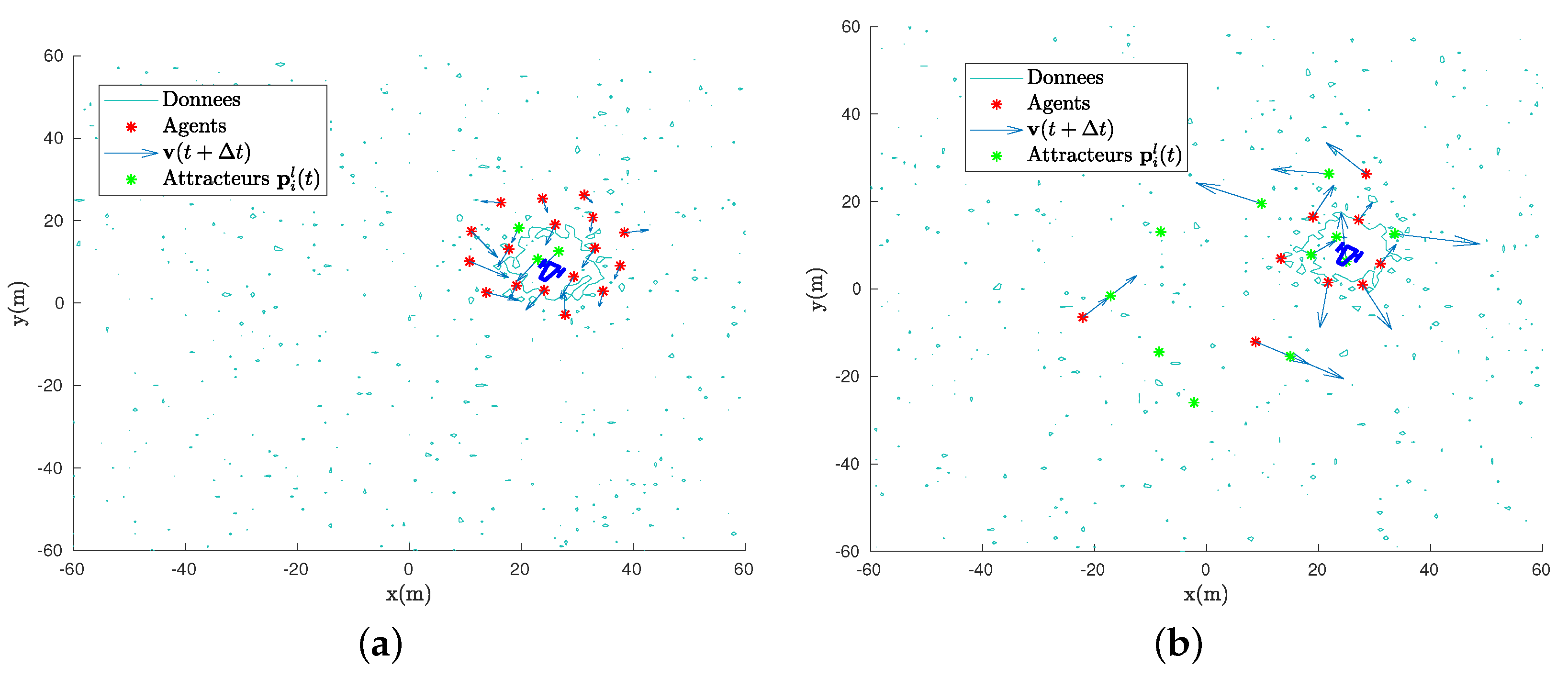
4.6.2. Communication Constraints

Obviously, communication constraints within the swarm yield to a limitation of our system: for example, our N agents will only be able to communicate with certain other agents, which will multiply the number of attractors and behaviors. We have different phenomena that will constrain the swarm:

• Isolation of individuals: if, at any given time, one or more agents make bad choices, they may be unable to communicate with anyone, and consequently they will be unable to move following Equation (18).
• Emergence of subgroups: two opposite attractors in the group can lead to the fission of the group where all the agents are connected in two or more subgroups, so there is no more direct or indirect link between any agent i and j.

We illustrate these cases in Figure 5, with the illustration of an efficient tracking of a source, in Figure 5a, and a less efficient tracking, in Figure 5b. The source follows the environment function (1) after $t=100$ s. We can see the importance of the setting of $r_{eq}$ compared to $r_{com}$. In Figure 5b, we can see the isolated agents, which are attracted by themselves, and consequently unable to move, and sub-groups of 2 robots, which are unable to track the target because they are too few. We will discuss in Section 5 the choice of these parameters, since it is directly related to the tracking performance of the target.

5. Results

To measure the evolution of tracking, we use the metric $D_{100}=∥\overline{\mathbf{p}}-{\mathbf{p}}_s∥$, a derivative of the $D_{25}$ metric used in [40]. ${\mathbf{p}}_s\left(t\right)$ is the target’s position, and $D_{100}$ is the distance between the center of gravity and the position of the source. Subscript 100 defines the fact that $100\%$ of the swarm elements are taken into account. If $D_{100}>>r_{max}·r_{eq}$, we will logically consider that the target tracking is “bad” and failed. If $0<D_{100}<r_{max}·r_{eq}$, we consider that the tracking is “good”.

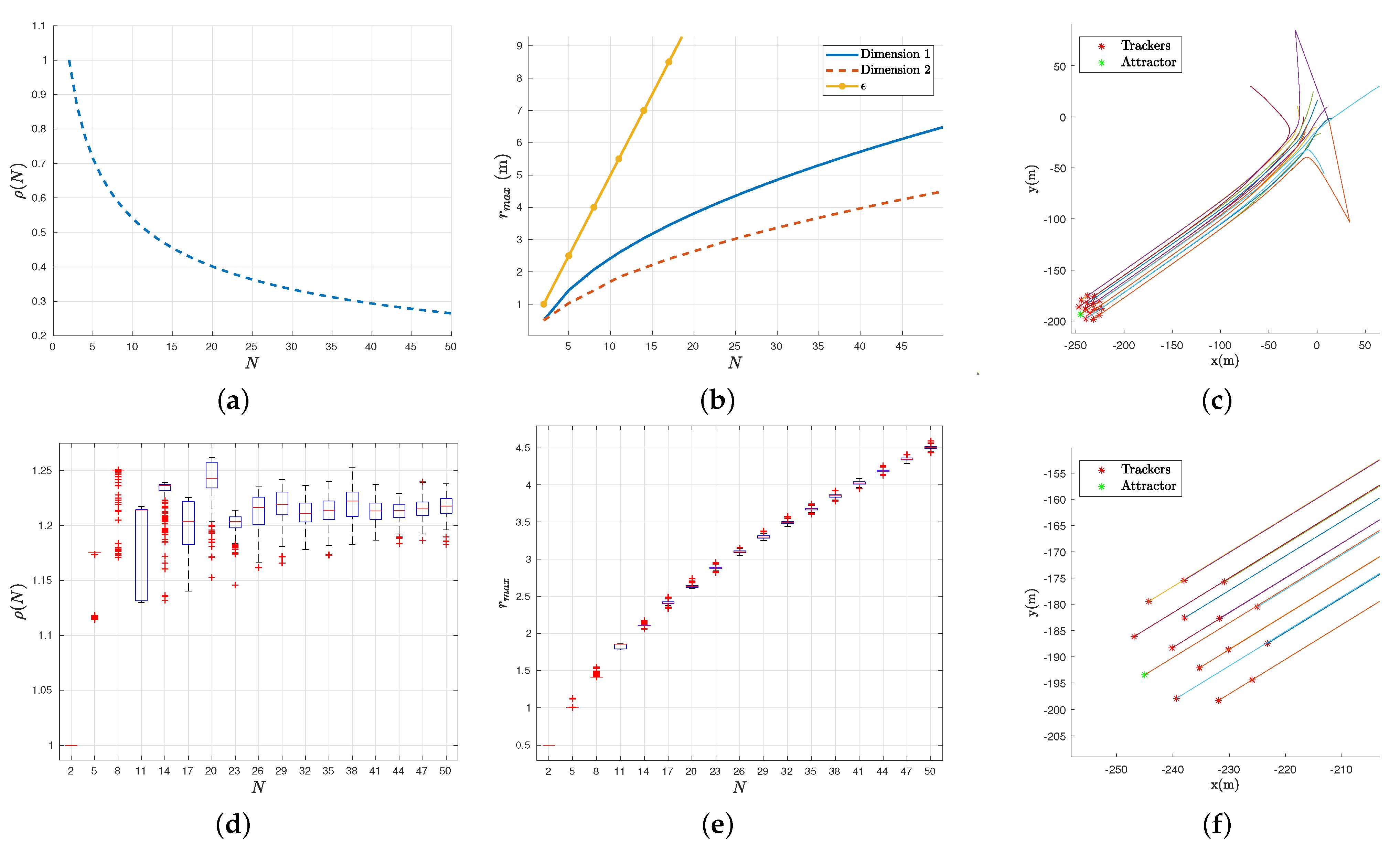
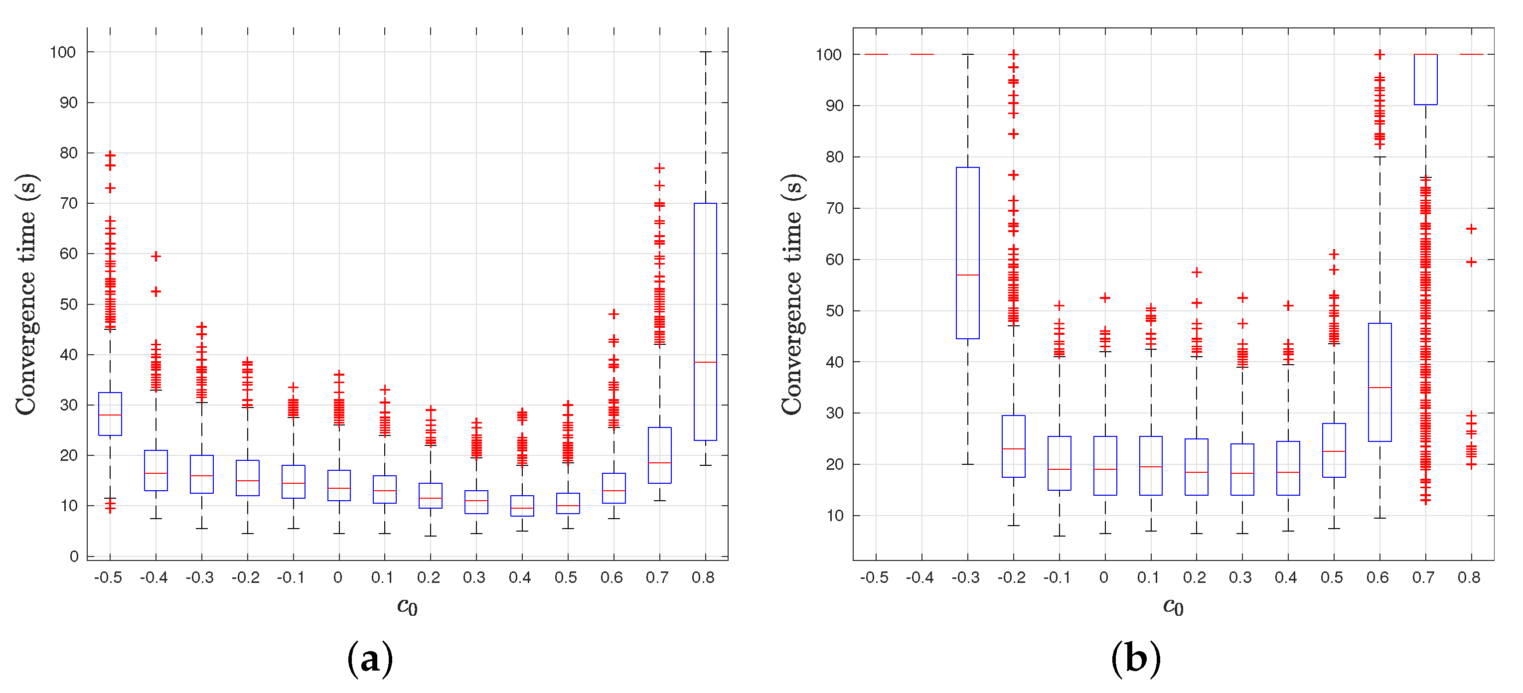
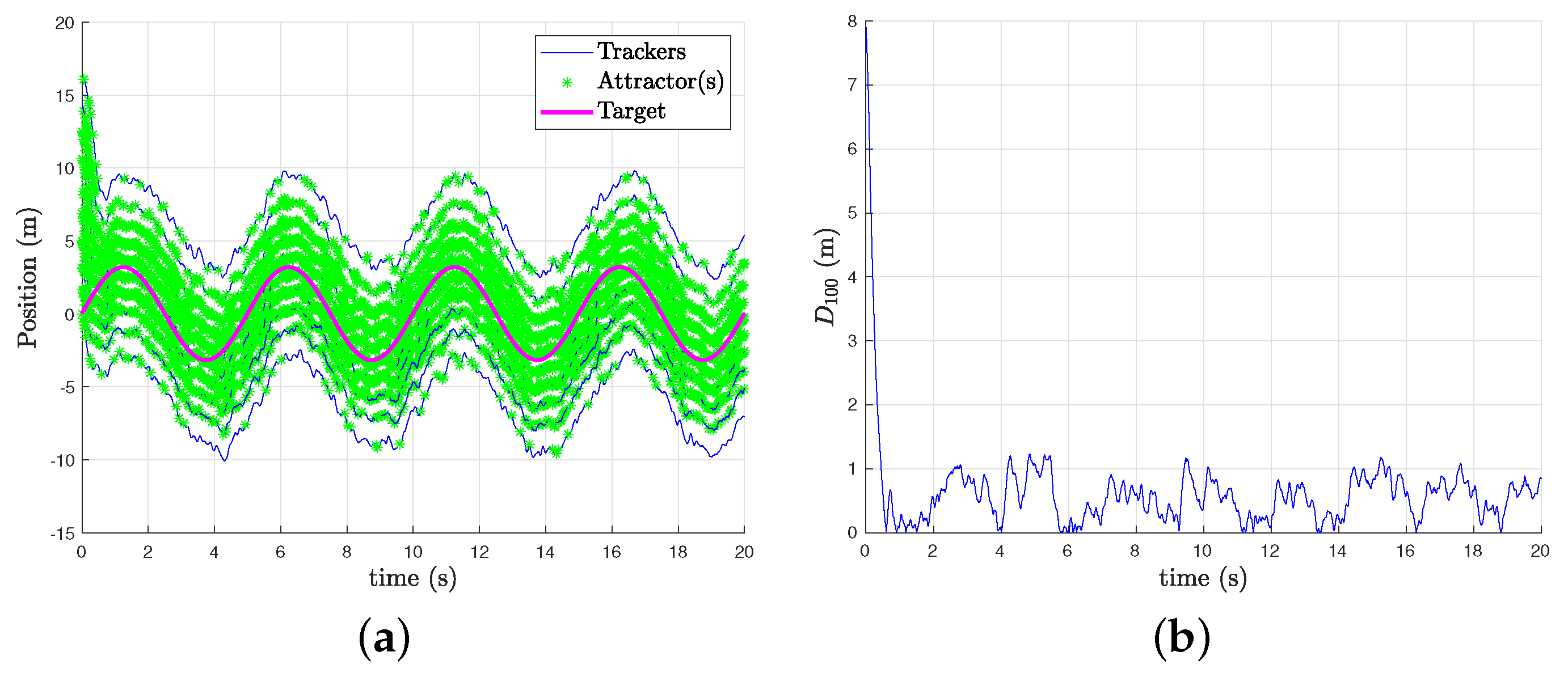
5.1. Dimension 1

The trackers measure information released by the dynamic source following environment Equation (1) without temporal decrease ($\tau \to +\infty$). An attractor is represented by green stars in Figure 6. It is the agent with the highest information measured at time t within its communication limits.

The target follows a periodic trajectory. Its speed follows a cosine function with a period $T=\frac{t_{max}}{4}$, with $t_{max}$ the simulation time. In Figure 6, we illustrate such a tracking scenario with agents which follow LCPSO Equation (18). The distance between the swarm center of gravity and the source $D_{100}$ oscillates because the number of attractors and their position change at each time step. However, the swarm is still centred on the target when $t\ge 1$ s, with en error limited in space ($D_{100}\le 1.5$ m with $r_{max}$ larger than 7 m).

In Figure 7, we illustrate the average of $D_{100}$ during the whole simulation as a function of $r_{eq}$ and $r_{com}$ in dimension 1. We have used a Monte-Carlo method with 100 samples. We can observe in the simulation results that the target tracking is inefficient when $r_{eq}\ge \frac{8}{10}{r}_{com}$ (between “bad” and “correct” results), but is efficient elsewhere. Farther are parameters away from this limitation, better are the results.

5.2. Dimension 2

In Dimension 2, we have already performed an analysis on target tracking in a previous article [40]. We have shown in simulation results that the LCPSO algorithm was relevant to track an underwater mobile target with communication constraints [40]. A maximal speed constraint is necessary, arbitrarily set to $v_{max}=5$ m.s${}^{-1}$, because the capacities to lose the swarm must be controlled. We extend the work made in this article studying two types of trajectories for the source to illustrate their impact on tracking performances:

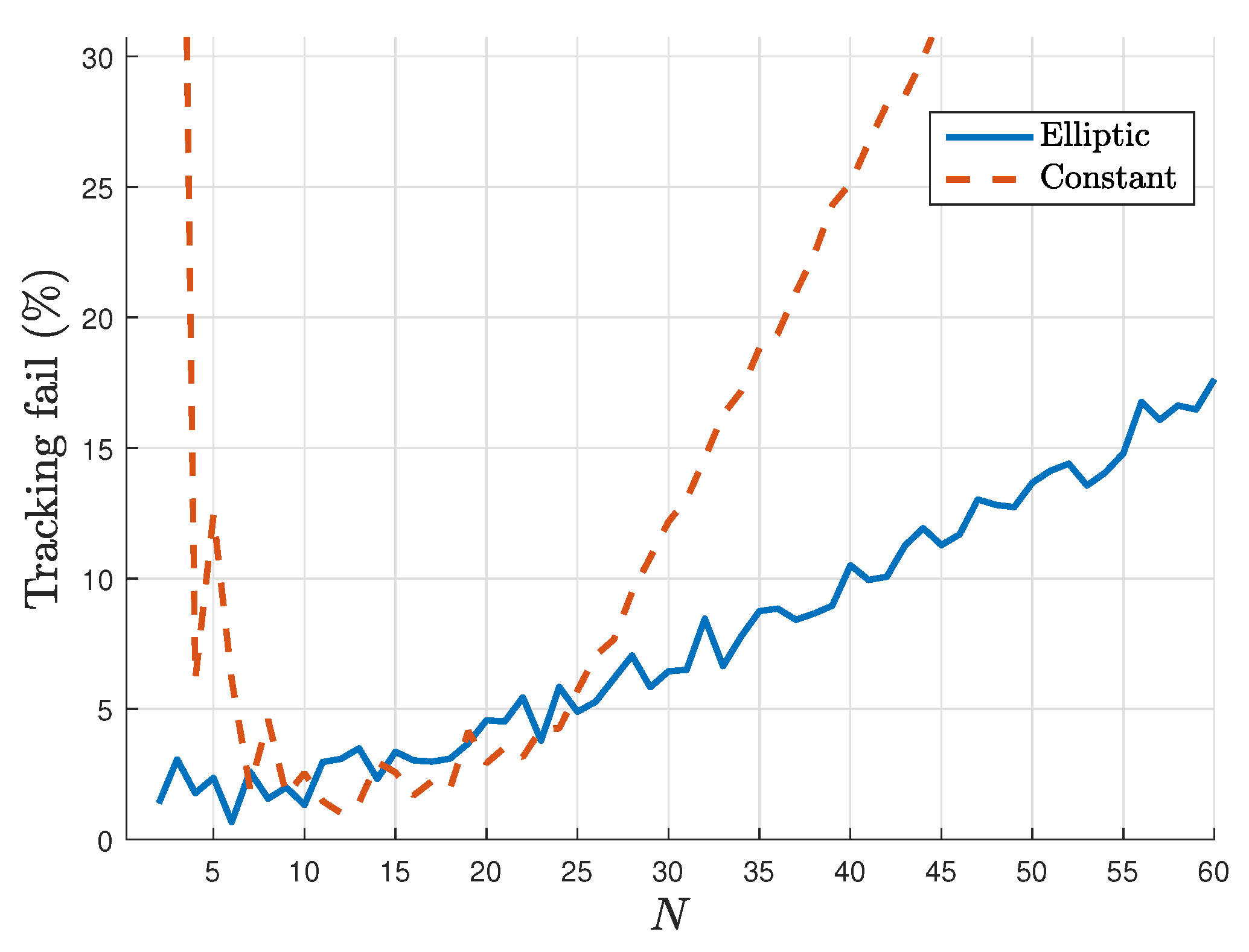
• The source follows an elliptical trajectory, centered on ${(0,0)}^T$, with radius $L_x=15$ m and $L_y=10$ m and initial position at point ${(-40,-40)}^T$. This choice is arbitrary, but the important thing is to see how the swarm reacts with violent heading changes, periodically coming back in the area that the agents are monitoring. The speed of the source oscillates between 2 and 4 m.s${}^{-1}$.
• The source has a constant trajectory, that is, a constant heading. It always starts from the point ${(-40,-40)}^T$, with a speed of 3 m.s${}^{-1}$ and a heading of 0.8 rad. The heading is chosen to cross the area monitored by our agents.

We can see in Figure 8 that when $N>15$, the tracking fail percentage increases gradually, especially for the constant trajectory. This is due to the environment function f: if some agents are too far from the source, they will only be able to measure the noise; and, even worse, this will also be the case for their neighbors. Consequently, the swarm will be dislocated into packets. This phenomenon is illustrated in Figure 5b. In the case of a constant trajectory, the isolated agents have very little chance of finding the group that succeeds in tracking it, unlike the elliptical trajectory where the source comes back. Thus, with communication restrictions, it is necessary to limit the number of agents that will track the source, in order to have better tracking performance and do not waste resources; we can see that between 10 and 15 agents, the source tracking is optimal whatever its trajectory.

We add Figure 9 to give an operational point of view of our algorithm, as a function of $r_{com}$ and $r_{eq}$, with the same parameters [40]. With the help of Figure 8, the number of agents is fixed to $N=10$. In Figure 9, we can observe more restrictions than in dimension 1. Indeed, there is an area where a too low $r_{eq}$ degrades the results whatever $r_{com}$, because agents are too close from each other, and the swarm is unable to have a stable formation. There are also more important restrictions on communication limits, in comparison with Dimension 1. Indeed, if $r_{eq}$ is too much important compared to $r_{com}$, the number of isolated agents increases and the swarm is unable to track the target. Under this limit, some agents can lose the group, but without consequences on tracking performances, as illustrated in Figure 5b.

6. Conclusions

In this paper, we carried out an analysis of LCPSO algorithm that merges the spirit of PSO and flocking algorithms. This analysis is supported by mathematical theorems, that apply regardless of the dimension, or when necessary, by Monte-Carlo results, especially concerning communication constraints. Using only one attractor in a limited area permits to follow a target accurately. We summarise the contributions of this paper by the following points.

First, the formation at equilibrium is resilient to communication limits and the brutal moves of the target because Equation (18) is only based on measurements at time t. Moreover, we have proven analytically that the formation will stay stable in the sense of Definition 2 whatever the dimension and the place of the attractor(s) in the swarm. The strength of this formation avoids collisions between agents and losing agents with communication constraints. Finally, the speed is intrinsically limited and predictable thanks to Equation (17).

The stability of the swarm formation whatever the conditions (communication limits and the behavior of the target) makes our algorithm applicable in very constrained environments, like underwater scenario for example. LCPSO algorithm is resilient to the breakdown of some agents because the attractor depends on measurements and can be exchanged easily with another agent. Communication limits do not degrade our swarm formation, and the simplicity of LCPSO allows the robot to embed only few computing power.

Our work still has many limitations, which we acknowledge here. First, the plume model should be modified to be more realistic [31,43] to include the problem of measurement noise with a low SNR and the problem of noise correlation (in our case the measurement noise was uncorrelated in time and space). Second, we left out some constraints in our algorithm. For instance, we do not consider localization problems of agents with real sensors: while an exact absolute position is not important for our algorithm, a correct relative position is still necessary. This is an issue in the underwater environment, for instance. However, better positioning in challenging environments can often be enhanced using techniques such as Simultaneous Localization And Mapping (SLAM) [49,50] using variants of Kalman filters [48] or Interval Analysis [51] to take position uncertainty into account; our work can integrate these methods. Third, robotic constraints on the motion of agents could be applied on our model, in particular for heading and speed or with a linearisation of the agents’ trajectory [12]. Finally, we only used information in a scalar form. If we considered, when feasible, non-scalar information, resolving our problem could be easier. For example, we could measure a local gradient for function f to indicate the direction of its maximum. All of these limitations and possible solutions are left out for future work.

References

- Gueron, S.; Levin, S.A.; Rubenstein, D. The Dynamics of Herds: From Individuals to Aggregations. J. Theoret. Biol. 1996, 182, 85–98. [Google Scholar] [CrossRef]
- Camazine, S.; Franks, N.R.; Sneyd, J.; Bonabeau, E.; Deneubourg, J.L.; Theraula, G. Self-Organization in Biological Systems; Princeton University Press: Princeton, NJ, USA, 2001. [Google Scholar]
- Ballerini, M.; Cabibbo, N.; Candelier, R.; Cavagna, A.; Cisbani, E.; Giardina, I.; Lecomte, V.; Orlandi, A.; Parisi, G.; Procaccini, A.; et al. Interaction Ruling Animal Collective Behaviour Depends on Topological rather than Metric Distance: Evidence from a Field Study. Proc. Natl. Acad. Sci. USA 2008, 105, 1232–1237. [Google Scholar] [CrossRef] [PubMed]
- Pitcher, T.J.; Wyche, C.J. Predator-avoidance behaviours of sand-eel schools: Why schools seldom split. In Predators and Prey in Fishes, Proceedings of the 3rd Biennial Conference on the Ethology and Behavioral Ecology of Fishes, Normal, IL, USA, 19–22 May 1981; Noakes, D.L.G., Lindquist, D.G., Helfman, G.S., Ward, J.A., Noakes, D.L.G., Lindquist, D.G., Helfman, G.S., Ward, J.A., Eds.; Springer: Dordrecht, The Netherlands, 1983; pp. 193–204. [Google Scholar]
- Lopez, U.; Gautrais, J.; Couzin, I.D.; Theraulaz, G. From behavioural analyses to models of collective motion in fish schools. Interface Focus 2012, 2, 693–707. [Google Scholar] [CrossRef] [PubMed]
- Dorigo, M.; Birattari, M.; Stutzle, T. Ant colony optimization. IEEE Comput. Intell. Mag. 2006, 1, 28–39. [Google Scholar] [CrossRef]
- Bechinger, C.; Di Leonardo, R.; Löwen, H.; Reichhardt, C.; Volpe, G.; Volpe, G. Active particles in complex and crowded environments. Rev. Mod. Phys. 2016, 88, 045006. [Google Scholar] [CrossRef]
- Carrillo, J.A.; Choi, Y.P.; Perez, S.P. A Review on Attractive–Repulsive Hydrodynamics for Consensus in Collective Behavior. In Active Particles, Volume 1: Advances in Theory, Models, and Applications; Bellomo, N., Degond, P., Tadmor, E., Choi, Y.P., Eds.; Springer: Cham, Switzerland, 2017; pp. 259–298. [Google Scholar]
- Vásárhelyi, G.; Virágh, C.; Somorjai, G.; Nepusz, T.; Eiben, A.E.; Vicsek, T. Optimized flocking of autonomous drones in confined environments. Sci. Robot. 2018, 3, eaat3536. [Google Scholar] [CrossRef]
- Reynolds, C.W. Flocks, Herds and Schools: A Distributed Behavioral Model. SIGGRAPH Comput. Graph. 1987, 21, 25–34. [Google Scholar] [CrossRef]
- Tanner, H.G.; Jadbabaie, A.; Pappas, G.J. Stable flocking of mobile agents, Part I: Fixed topology. In Proceedings of the 42nd IEEE International Conference on Decision and Control (IEEE Cat. No. 03CH37475), Maui, HI, USA, 9–12 December 2003; Volume 2, pp. 2010–2015. [Google Scholar]
- Tanner, H.G.; Jadbabaie, A.; Pappas, G.J. Stable flocking of mobile agents, Part II: Dynamic topology. In Proceedings of the 42nd IEEE International Conference on Decision and Control (IEEE Cat. No. 03CH37475), Maui, HI, USA, 9–12 December 2003; Volume 2, pp. 2016–2021. [Google Scholar]
- Pugh, J.; Martinoli, A. Inspiring and Modeling Multi-Robot Search with Particle Swarm Optimization. In Proceedings of the 2007 IEEE Swarm Intelligence Symposium, Honolulu, HI, USA, 1–5 April 2007; pp. 332–339. [Google Scholar]
- Xue, S.; Zhang, J.; Zeng, J. Parallel asynchronous control strategy for target search with swarm robots. Int. J. Bio-Inspired Comput. 2009, 1, 151–163. [Google Scholar] [CrossRef]
- Liu, Z.; Xue, S.; Zeng, J.; Zhao, J.; Zhang, G. An evaluation of PSO-type swarm robotic search: Modeling method and controlling properties. In Proceedings of the 2010 International Conference on Networking, Sensing and Control (ICNSC), Chicago, IL, USA, 10–12 April 2010; pp. 360–365. [Google Scholar]
- La, H.M.; Sheng, W. Adaptive flocking control for dynamic target tracking in mobile sensor networks. In Proceedings of the 2009 IEEE/RSJ International Conference on Intelligent Robots and Systems, St. Louis, MO, USA, 11–15 October 2009; pp. 4843–4848. [Google Scholar] [CrossRef]
- Kwa, H.L.; Leong Kit, J.; Bouffanais, R. Optimal Swarm Strategy for Dynamic Target Search and Tracking. In Proceedings of the 19th International Conference on Autonomous Agents and MultiAgent Systems, Auckland, New Zealand, 9–13 May 2020. [Google Scholar]
- Kumar, A.S.; Manikutty, G.; Bhavani, R.R.; Couceiro, M.S. Search and rescue operations using robotic darwinian particle swarm optimization. In Proceedings of the 2017 International Conference on Advances in Computing, Communications and Informatics (ICACCI), Udupi, India, 13–16 September 2017; pp. 1839–1843. [Google Scholar]
- Marques, L.; Nunes, U.; de Almeida, A.T. Particle swarm-based olfactory guided search. Auton. Robot. 2006, 20, 277–287. [Google Scholar] [CrossRef]
- Jatmiko, W.; Sekiyama, K.; Fukuda, T. A PSO-based mobile robot for odor source localization in dynamic advection-diffusion with obstacles environment: Theory, simulation and measurement. IEEE Comput. Intell. Mag. 2007, 2, 37–51. [Google Scholar] [CrossRef]
- Jatmiko, W.; Pambuko, W.; Mursanto, P.; Muis, A.; Kusumoputro, B.; Sekiyama, K.; Fukuda, T. Localizing multiple odor sources in dynamic environment using ranged subgroup PSO with flow of wind based on open dynamic engine library. In Proceedings of the 2009 International Symposium on Micro-NanoMechatronics and Human Science, Nagoya, Japan, 8–11 November 2009; pp. 602–607. [Google Scholar]
- Sinha, A.; Kumar, R.; Kaur, R.; Mishra, R.K. Consensus-Based Odor Source Localization by Multiagent Systems under Resource Constraints. IEEE Trans. Cybern. 2019, 50, 3254–3263. [Google Scholar] [CrossRef] [PubMed]
- Fu, Z.; Chen, Y.; Ding, Y.; He, D. Pollution Source Localization Based on Multi-UAV Cooperative Communication. IEEE Access 2019, 7, 29304–29312. [Google Scholar] [CrossRef]
- Lu, Q.; Han, Q.L. A Probability Particle Swarm Optimizer with Information-Sharing Mechanism for Odor Source Localization. IFAC Proc. Vol. 2011, 44, 9440–9445. [Google Scholar] [CrossRef]
- Lu, Q.; Han, Q.; Xie, X.; Liu, S. A Finite-Time Motion Control Strategy for Odor Source Localization. IEEE Trans. Ind. Electron. 2014, 61, 5419–5430. [Google Scholar]
- Lu, Q.; Han, Q.; Liu, S. A Cooperative Control Framework for a Collective Decision on Movement Behaviors of Particles. IEEE Trans. Evol. Comput. 2016, 20, 859–873. [Google Scholar] [CrossRef]
- Kennedy, J.; Eberhart, R. Particle swarm optimization. In Proceedings of the ICNN’95—International Conference on Neural Networks, Perth, Australia, 27 November–1 December 1995; Volume 4, pp. 1942–1948. [Google Scholar]
- Yang, J.; Wang, X.; Bauer, P. Extended PSO Based Collaborative Searching for Robotic Swarms With Practical Constraints. IEEE Access 2019, 7, 76328–76341. [Google Scholar] [CrossRef]
- Poli, R.; Kennedy, J.; Blackwell, T. Particle swarm optimization—An Overview. Swarm Intell. 2007, 1. [Google Scholar] [CrossRef]
- Zarzhitsky, D.; Spears, D.; Thayer, D. Experimental studies of swarm robotic chemical plume tracing using computations fluid dynamics simulations. Int. J. Intell. Comput. Cybern. 2010, 3. [Google Scholar] [CrossRef]
- Farrell, J.; Murlis, J.; Long, X.; Li, W.; Cardé, R. Filament-Based Atmospheric Dispersion Model to Achieve Short Time-Scale Structure of Odor Plumes. Environ. Fluid Mech. 2002, 2, 143–169. [Google Scholar] [CrossRef]
- Hettiarachchi, S.; Spears, W.M. Distributed adaptive swarm for obstacle avoidance. Int. J. Intell. Comput. Cybern. 2009, 2, 644–671. [Google Scholar] [CrossRef]
- Liu, A.H.; Bunn, J.J.; Chandy, K.M. Sensor networks for the detection and tracking of radiation and other threats in cities. In Proceedings of the 10th ACM/IEEE International Conference on Information Processing in Sensor Networks, Chicago, IL, USA, 12–14 April 2011; pp. 1–12. [Google Scholar]
- Liu, Z.; Smith, P.; Park, T.; Trindade, A.A.; Hui, Q. Automated Contaminant Source Localization in Spatio-Temporal Fields: A Response Surface and Experimental Design Approach. IEEE Trans. Syst. Man Cybern. Syst. 2017, 47, 569–583. [Google Scholar] [CrossRef]
- Briñon Arranz, L. Cooperative Control Design for a Fleet of AUVs under Communication Constraints. Ph.D. Thesis, Université de Grenoble, Saint-Martin-d’Hères, France, 2011. [Google Scholar]
- Tian, Y.; Li, W.; Zhang, F. Moth-inspired plume tracing via autonomous underwater vehicle with only a pair of separated chemical sensors. In Proceedings of the OCEANS 2015—MTS/IEEE, Washington, DC, USA, 19–22 October 2015; pp. 1–8. [Google Scholar]
- Lochmatter, T. Bio-Inspired and Probabilistic Algorithms for Distributed Odor Source Localization Using Mobile Robots. Ph.D. Thesis, Ecole Polytechnique Federale de Lausanne, Lausanne, Switzerland, 2010; p. 135. [Google Scholar]
- Mogilner, A.; Edelstein-Keshet, L.; Bent, L.; Spiros, A. Mutual interactions, potentials, and individual distance in a social aggregation. J. Math. Biol. 2003, 47, 353–389. [Google Scholar] [CrossRef] [PubMed]
- Gazi, V.; Passino, K.M. Swarm Stability and Optimization, 1st ed.; Springer: Berlin, Germany, 2011. [Google Scholar]
- Coquet, C.; Aubry, C.; Arnold, A.; Bouvet, P. A Local Charged Particle Swarm Optimization to track an underwater mobile source. In Proceedings of the OCEANS 2019, Marseille, France, 17–20 June 2019; pp. 1–7. [Google Scholar] [CrossRef]
- Stojanovic, M.; Beaujean, P.P.J. Acoustic Communication. In Springer Handbook of Ocean Engineering; Dhanak, M.R., Xiros, N.I., Eds.; Springer: Cham, Switzerland, 2016; pp. 359–386. [Google Scholar]
- Hosseinzadeh, M. Chapter 22—UAV geofencing: Navigation of UVAs in constrained environments. In Unmanned Aerial Systems; Koubaa, A., Azar, A.T., Eds.; Advances in Nonlinear Dynamics and Chaos (ANDC); Academic Press: Cambridge, MA, USA, 2021; pp. 567–594. [Google Scholar] [CrossRef]
- Chen, X.; Huang, J. Odor source localization algorithms on mobile robots: A review and future outlook. Robot. Auton. Syst. 2019, 112, 123–136. [Google Scholar] [CrossRef]
- Cleghorn, C.W.; Engelbrecht, A.P. Particle swarm stability: A theoretical extension using the non-stagnate distribution assumption. Swarm Intell. 2018, 12, 1–22. [Google Scholar] [CrossRef]
- Van Den Bergh, F. An Analysis of Particle Swarm Optimizers. Ph.D. Thesis, University of Pretoria South Africa, Pretoria, South Africa, 2002. [Google Scholar]
- Olfati-Saber, R. Flocking for multi-agent dynamic systems: Algorithms and theory. IEEE Trans. Autom. Control 2006, 51, 401–420. [Google Scholar] [CrossRef]
- Borzì, A.; Wongkaew, S. Modeling and control through leadership of a refined flocking system. Math. Model. Methods Appl. Sci. 2015, 25, 255–282. [Google Scholar] [CrossRef]
- Jaulin, L. Mobile Robotics; The MIT Press: Cambridge, MA, USA, 2015. [Google Scholar]
- Durrant-Whyte, H.; Bailey, T. Simultaneous localization and mapping: Part I. IEEE Robot. Autom. Mag. 2006, 13, 99–110. [Google Scholar] [CrossRef]
- Bailey, T.; Durrant-Whyte, H. Simultaneous localization and mapping (SLAM): Part II. IEEE Robot. Autom. Mag. 2006, 13, 108–117. [Google Scholar] [CrossRef]
- Soares, G.L.; Arnold-Bos, A.; Jaulin, L.; Maia, C.A.; Vasconcelos, J.A. An Interval-Based Target Tracking Approach for Range-Only Multistatic Radar. IEEE Trans. Magn. 2008, 44, 1350–1353. [Google Scholar] [CrossRef]
Samples of the compounds are available from the authors. |
Publisher’s Note: MDPI stays neutral with regard to jurisdictional claims in published maps and institutional affiliations. |
© 2021 by the authors. Licensee MDPI, Basel, Switzerland. This article is an open access article distributed under the terms and conditions of the Creative Commons Attribution (CC BY) license (https://creativecommons.org/licenses/by/4.0/).
Share and Cite
Coquet, C.; Arnold, A.; Bouvet, P.-J. Control of a Robotic Swarm Formation to Track a Dynamic Target with Communication Constraints: Analysis and Simulation. Appl. Sci. 2021, 11, 3179. https://doi.org/10.3390/app11073179
Coquet C, Arnold A, Bouvet P-J. Control of a Robotic Swarm Formation to Track a Dynamic Target with Communication Constraints: Analysis and Simulation. Applied Sciences. 2021; 11(7):3179. https://doi.org/10.3390/app11073179
Chicago/Turabian StyleCoquet, Charles, Andreas Arnold, and Pierre-Jean Bouvet. 2021. "Control of a Robotic Swarm Formation to Track a Dynamic Target with Communication Constraints: Analysis and Simulation" Applied Sciences 11, no. 7: 3179. https://doi.org/10.3390/app11073179
APA StyleCoquet, C., Arnold, A., & Bouvet, P.-J. (2021). Control of a Robotic Swarm Formation to Track a Dynamic Target with Communication Constraints: Analysis and Simulation. Applied Sciences, 11(7), 3179. https://doi.org/10.3390/app11073179