
Automated Ground Truth Generation for Learning-Based Crack Detection on Concrete Surfaces


Abstract
:1. Introduction
- We introduce an algorithm that can perform automated data labeling for concrete images exhibiting cracks. This algorithm first produces preliminary labels via several image processing procedures. Hence, the preliminary labels, namely, the first-round GTs, are used to train a deep U-Net-based model.
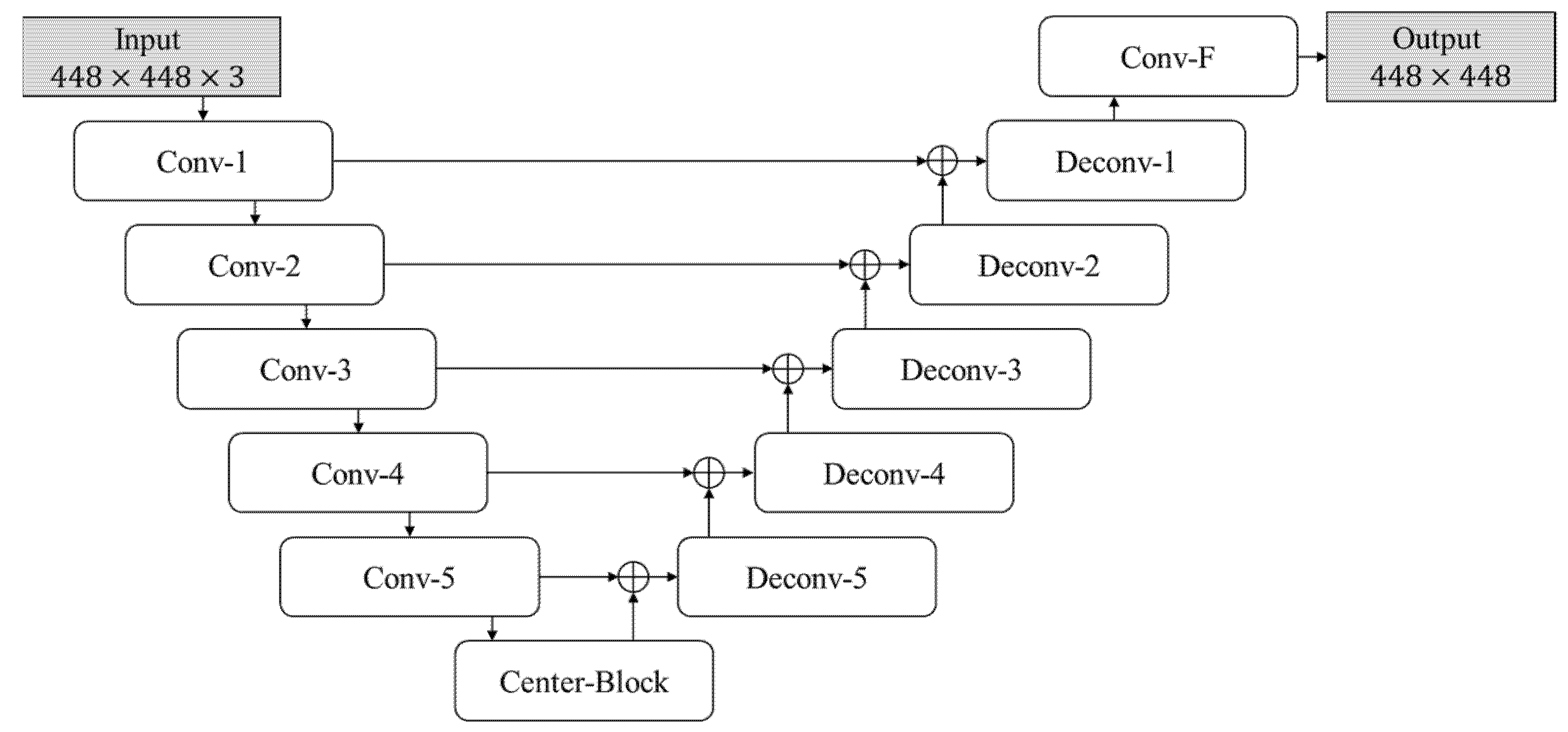
- The U-Net-based model above is implemented by integrating the VGG16 into the U-Net to form the vanilla architecture of our proposed crack detection model. In addition, the encoder portion of this crack detection model is replaced by the well-known residual network (ResNet) for evaluating the effectiveness among different encoder backbones.
- We propose a scheme to refine the first-round GTs to generate refined (also known as second-round) GTs. Using a fuzzy inference system and using a crack image and its prediction result yielded by the proposed model as inputs, we can derive the degree of each pixel belonging to the crack class. Next, a thresholding operation is employed to determine whether a pixel is categorized as a crack or non-crack. Subsequently, the second-round GTs of the training data were obtained. Moreover, the aforementioned U-Net-based model can be retrained using the second-round GTs to achieve better performances.
2. Proposed Method
2.1. First-Round GT Generation
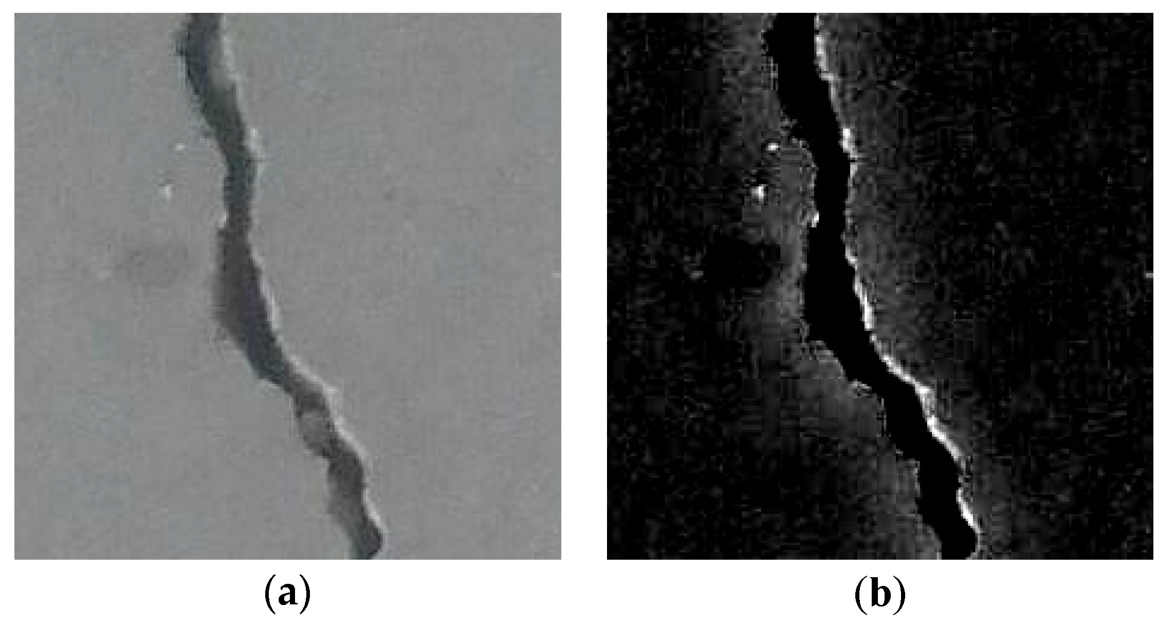
2.1.1. Edge Pixel Enhancement
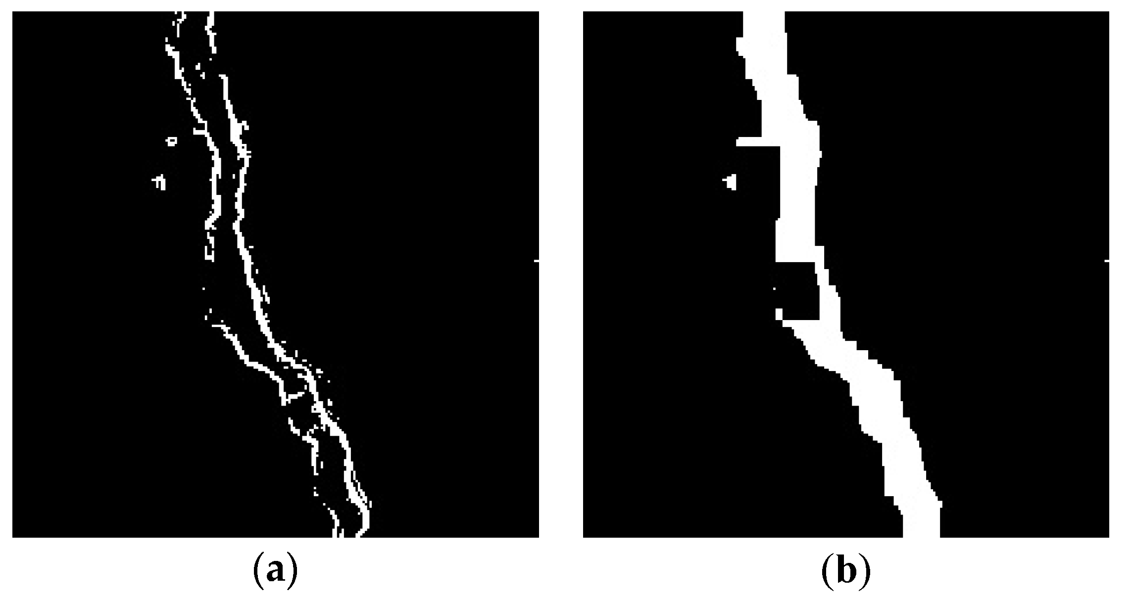
2.1.2. Crack Pixel Segmentation
2.2. Pre-Training Binary Segmentation Model for Crack Detection
2.3. Second-Round GT Generation: Refinement Stage
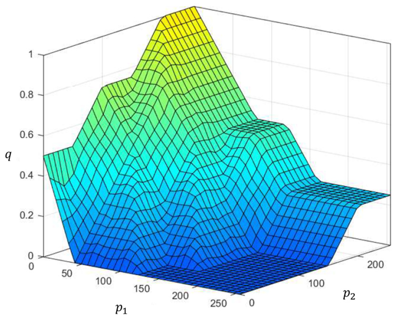
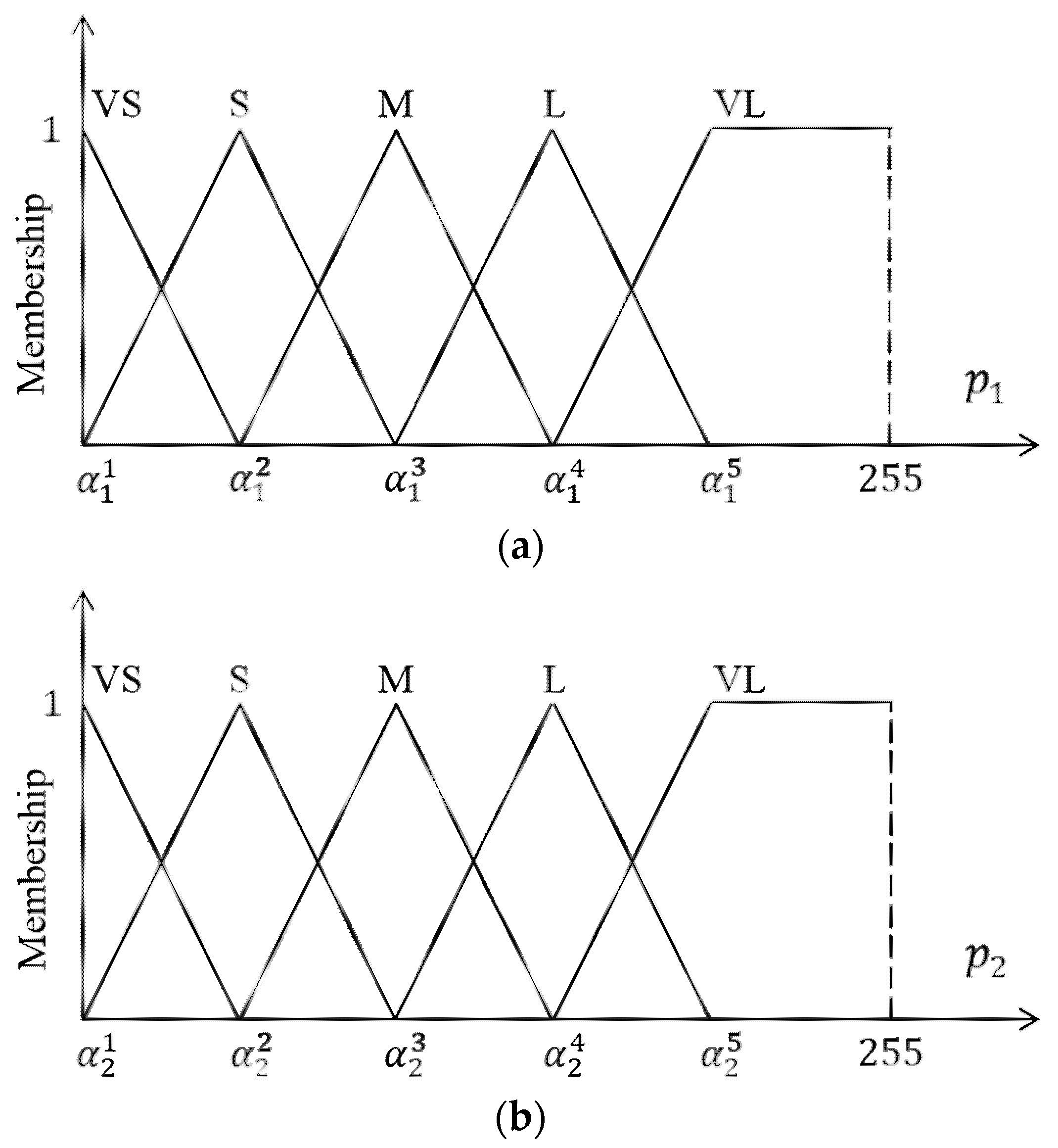
- Step 1: For a specified pixel , two inputs and are imported into the proposed FIS.
- Step 2: The non-fuzzy output is obtained using the fuzzy inference engine. This output is regarded as the degree to which pixel belongs to the crack or non-crack class.
- Step 3: Label the refined (second-round) GT, as expressed by
2.4. Main Procedure of Proposed Algorithm
| Algorithm 1: Automated Data Labeling for a Dataset |
| Input: All images in the dataset. Let be a specific image. |
| Output: Second-round GTs for all images. |
| Steps: |
| 1: Convert into a grayscale image . |
| 2: Apply Gaussian blur filter on , and obtain a blurred image . |
| 3: Subtract the blurred image from the gray image , denoted by . |
| 4: Perform Sobel edge detector on , and obtain the gradient magnitude and direction . |
| 5: Binarize the magnitude map by thresholding. |
| 6: Perform closing operation on this binarized map. |
| 7: Use connected-component labeling to obtain bounding boxes of cracks. |
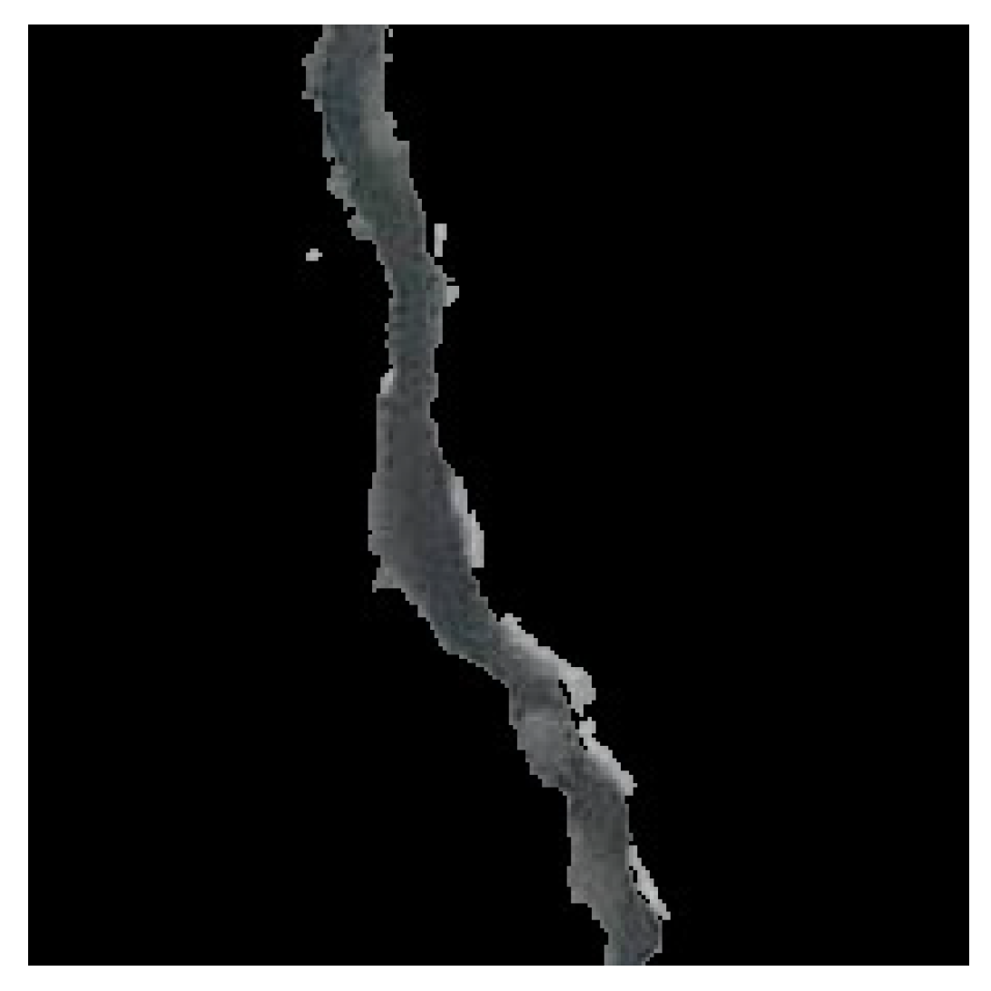
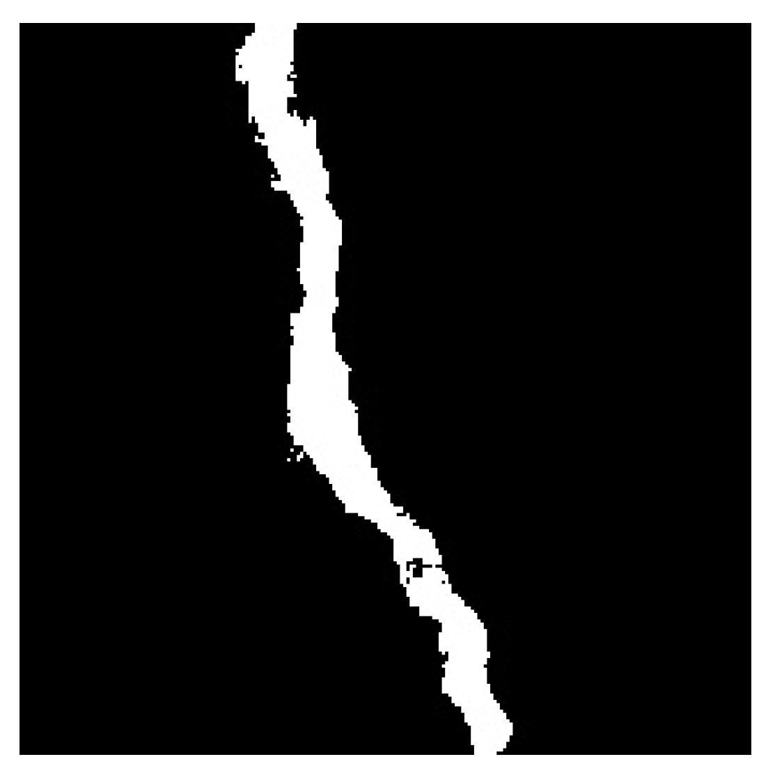
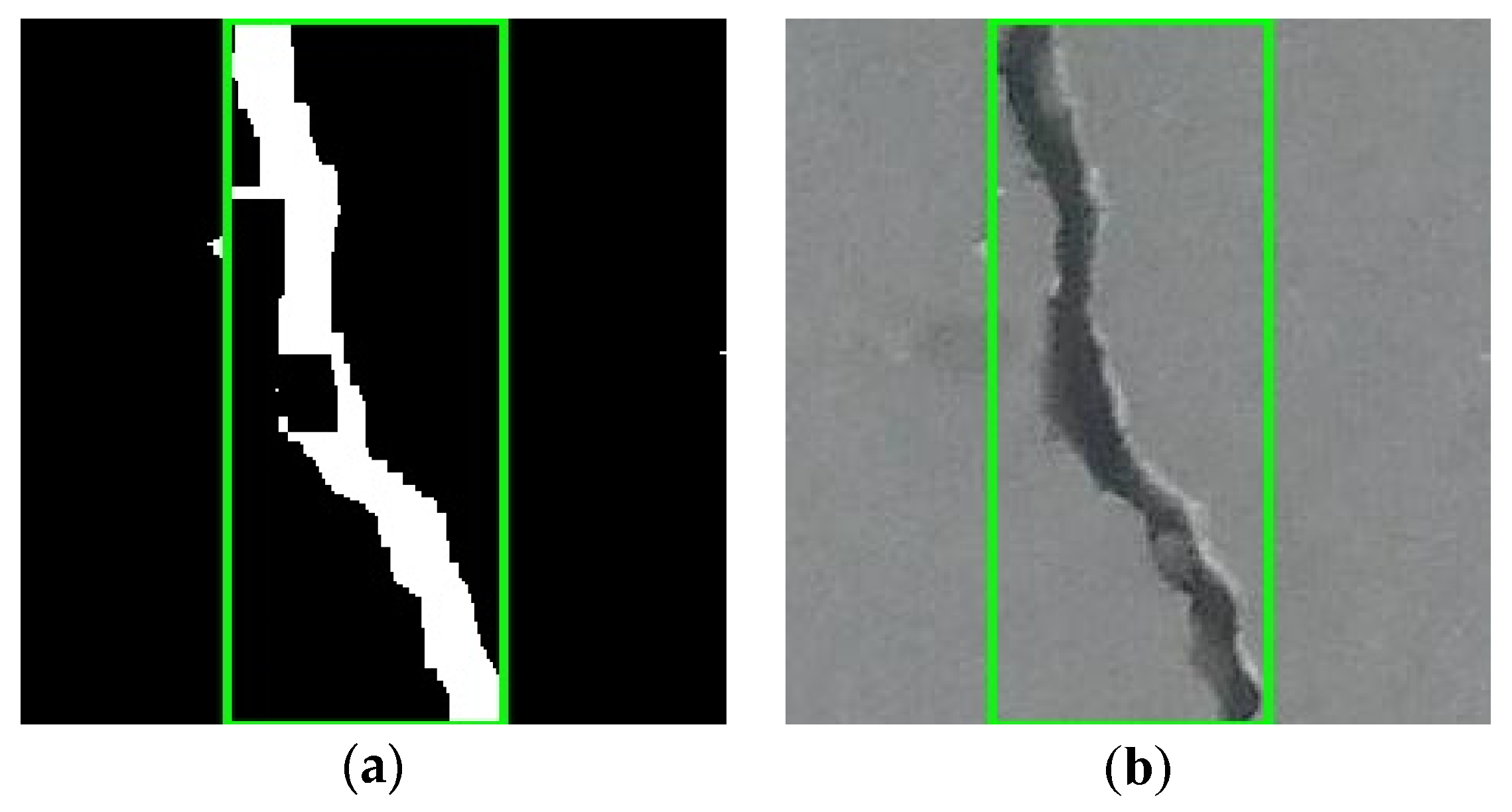
| 8: Apply GrabCut to extract crack pixels which are denoted by 1 in the first-round GT. |
| 9: Repeat Steps 1–8 for every image in the dataset. Collect training data, in which each sample consists of a pair of an image and its first-round GT. |
| 10: Pre-train a binary segmentation model using the training data obtained in Step 9. |
| 11: Obtain the prediction result for the image using this pre-trained model. |
| 12: Normalize to , in which every pixel value ranges from 0 to 255. |
| 13: Enhance the grayscale image to be by CLAHE. |
| 14: For every pixel in the image :Perform the proposed FIS to determine the degree to which pixel be longs to the crack or non-crack class. |
| 15: Repeat Steps 11–14 for every image in the dataset. The second-round GTs of all training samples are obtained. |
3. Implementation and Experiments
3.1. Crack Detection Models Based on U-Net
- Perform the algorithm of the first-round GT generation proposed in Section 2.1.
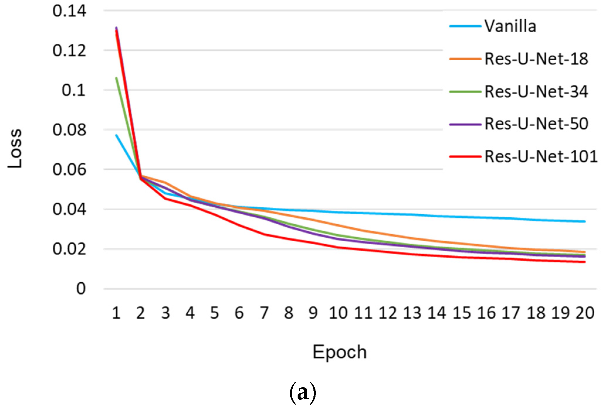
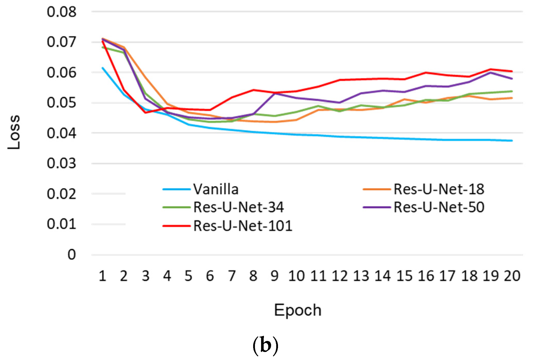
- Pre-train the U-Net-based models, including the vanilla, Res-U-Net-18, Res-U-Net-34, Res-U-Net-50, and Res-U-Net-101 models, separately. The hyper-parameters used during this training stage are the same as those introduced in Section 2.2.
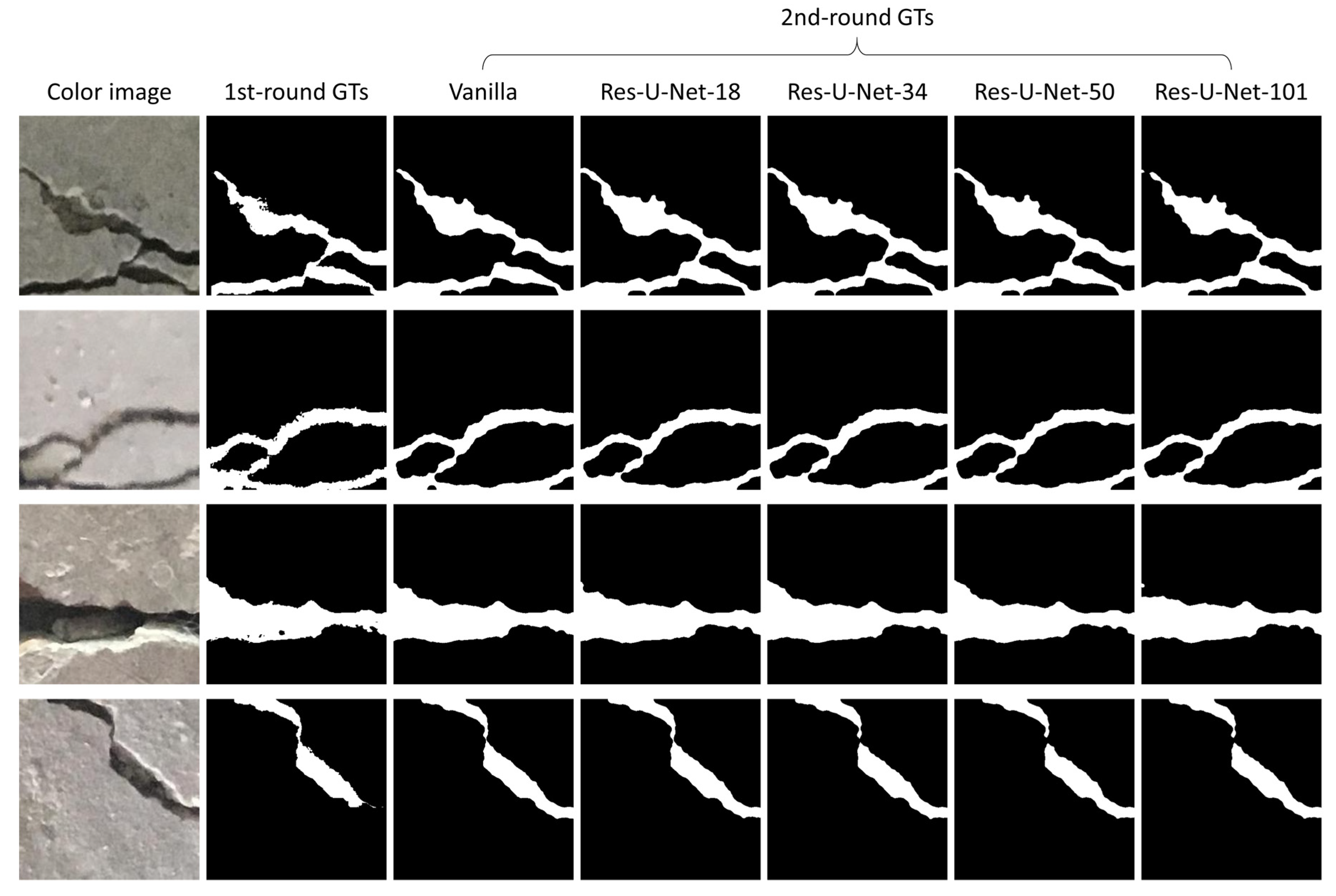
- Use each learned model to obtain the crack prediction results of the training data.
- On the basis of the prediction results, obtain the second-round GTs using the refinement scheme presented in Section 2.3.
- Finally, use the second-round GTs to re-train the five pre-trained models separately. Hence, U-Net-based crack detection models with different types of encoders are obtained.
3.2. Further Discussion on Computation of FIS
4. Quantitative Evaluation Using Different Datasets
5. Further Discussions and Improvements
6. Conclusions
Author Contributions
Funding
Institutional Review Board Statement
Informed Consent Statement
Data Availability Statement
Conflicts of Interest
References
- Ren, Y.; Huang, J.; Hong, Z.; Lu, W.; Yin, J.; Zou, L.; Shen, X. Image-based concrete crack detection in tunnels using deep fully convolutional networks. Constr. Build. Mater. 2020, 234, 117367. [Google Scholar] [CrossRef]
- Sirca, G.F., Jr.; Adeli, H. Infrared thermography for detecting defects in concrete structures. J. Civ. Eng. Manag. 2018, 24, 508–515. [Google Scholar] [CrossRef]
- Wolf, J.; Pirskawetz, S.; Zang, A. Detection of crack propagation in concrete with embedded ultrasonic sensors. Eng. Fract. Mech. 2015, 146, 161–171. [Google Scholar] [CrossRef]
- Cho, S.; Park, S.; Cha, G.; Oh, T. Development of image processing for crack detection on concrete structures through terrestrial laser scanning associated with the octree structure. Appl. Sci. 2018, 8, 2373. [Google Scholar] [CrossRef] [Green Version]
- Rabah, M.; Elhattab, A.; Fayad, A. Automatic concrete cracks detection and mapping of terrestrial laser scan data. NRIAG J. Astron. Geophys. 2013, 2, 250–255. [Google Scholar] [CrossRef] [Green Version]
- Turkan, Y.; Hong, J.; Laflamme, S.; Puri, N. Adaptive wavelet neural network for terrestrial laser scanner-based crack detection. Autom. Constr. 2018, 94, 191–202. [Google Scholar] [CrossRef] [Green Version]
- Giri, P.; Kharkovsky, S. Detection of surface crack in concrete using measurement technique with laser displacement sensor. IEEE Trans. Instrum. Meas. 2016, 65, 1951–1953. [Google Scholar] [CrossRef]
- Su, T.C. Application of computer vision to crack detection of concrete structure. Int. J. Eng. Technol. Innov. 2013, 5, 457. [Google Scholar] [CrossRef] [Green Version]
- Xu, H.; Tian, Y.; Lin, S.; Wang, S. Research of image segmentation algorithm applied to concrete bridge cracks. In Proceedings of the 2013 IEEE Third International Conference on Information Science and Technology (ICIST), Yangzhou, China, 23–25 March 2013. [Google Scholar]
- Nguyen, H.N.; Kam, T.Y.; Cheng, P.Y. An automatic approach for accurate edge detection of concrete crack utilizing 2D geometric features of crack. J. Signal Process. Syst. 2014, 77, 221–240. [Google Scholar] [CrossRef]
- Nishikawa, T.; Yoshida, J.; Sugiyama, T.; Fujino, Y. Concrete crack detection by multiple sequential image filtering. Comput.-Aided Civ. Infrastruct. Eng. 2012, 27, 29–47. [Google Scholar] [CrossRef]
- Prasanna, P.; Dana, K.; Gucunski, N.; Basily, B. Computer-vision based crack detection and analysis. In Proceedings of the Sensors and Smart Structures Technologies for Civil, Mechanical, and Aerospace Systems, San Diego, CA, USA, 12–15 March 2012. [Google Scholar]
- Cha, Y.J.; Choi, W.; Büyüköztürk, O. Deep learning-based crack damage detection using convolutional neural networks. Comput.-Aided Civ. Infrastruct. Eng. 2017, 32, 361–378. [Google Scholar] [CrossRef]
- Chen, F.C.; Jahanshahi, M.R. NB-CNN: Deep learning-based crack detection using convolutional neural network and Naïve Bayes data fusion. IEEE Trans. Ind. Electron. 2017, 65, 4392–4400. [Google Scholar] [CrossRef]
- Kim, B.; Cho, S. Automated vision-based detection of cracks on concrete surfaces using a deep learning technique. Sensors 2018, 18, 3452. [Google Scholar] [CrossRef] [Green Version]
- Long, J.; Shelhamer, E.; Darrell, T. Fully convolutional networks for semantic segmentation. In Proceedings of the IEEE Conference on Computer Vision and Pattern Recognition, Boston, MA, USA, 7–12 June 2015. [Google Scholar]
- Dung, C.V. Autonomous concrete crack detection using deep fully convolutional neural network. Autom. Constr. 2019, 99, 52–58. [Google Scholar] [CrossRef]
- Simonyan, K.; Zisserman, A. Very deep convolutional networks for large-scale image recognition. arXiv 2015, arXiv:1409.1556. [Google Scholar]
- Islam, M.M.; Kim, J.M. Vision-based autonomous crack detection of concrete structures using a fully convolutional encoder-decoder network. Sensors 2019, 19, 4251. [Google Scholar] [CrossRef] [Green Version]
- Zhang, J.; Lu, C.; Wang, J.; Wang, L.; Yue, X.G. Concrete cracks detection based on FCN with dilated convolution. Appl. Sci. 2019, 9, 2686. [Google Scholar] [CrossRef] [Green Version]
- He, K.; Zhang, X.; Ren, S.; Sun, J. Deep residual learning for image recognition. In Proceedings of the IEEE Conference on Computer Vision and Pattern Recognition, Las Vegas, NV, USA, 27–30 June 2016. [Google Scholar]
- Badrinarayanan, V.; Kendall, A.; Cipolla, R. Segnet: A deep convolutional encoder-decoder architecture for image segmentation. IEEE Trans. Pattern Anal. Mach. Intell. 2017, 39, 2481–2495. [Google Scholar] [CrossRef]
- Zou, Q.; Zhang, Z.; Li, Q.; Qi, X.; Wang, Q.; Wang, S. Deepcrack: Learning hierarchical convolutional features for crack detection. IEEE Trans. Image Process. 2018, 28, 1498–1512. [Google Scholar] [CrossRef]
- Ronneberger, O.; Fischer, P.; Brox, T. U-net: Convolutional networks for biomedical image segmentation. In Proceedings of the International Conference on Medical Image Computing and Computer-Assisted Intervention, Munich, Germany, 5–9 October 2015. [Google Scholar]
- Liu, Z.; Cao, Y.; Wang, Y.; Wang, W. Computer vision-based concrete crack detection using U-net fully convolutional networks. Autom. Constr. 2019, 104, 129–139. [Google Scholar] [CrossRef]
- Zhang, Y.; Chen, B.; Wang, J.; Li, J.; Sun, X. APLCNet: Automatic Pixel-Level Crack Detection Network Based on Instance Segmentation. IEEE Access 2020, 8, 199159–199170. [Google Scholar] [CrossRef]
- Li, S.; Zhao, X. Automatic crack detection and measurement of concrete structure using convolutional encoder-decoder network. IEEE Access 2020, 8, 134602–134618. [Google Scholar] [CrossRef]
- Zou, Y.; Zhang, Z.; Zhang, H.; Li, C.L.; Bian, X.; Huang, J.B.; Pfister, T. Pseudoseg: Designing pseudo labels for semantic segmentation. arXiv 2020, arXiv:2010.09713. [Google Scholar]
- Zhang, K.; Zhang, Y.; Cheng, H.D. Self-supervised structure learning for crack detection based on cycle-consistent generative adversarial networks. J. Comput. Civ. Eng. 2020, 34, 04020004. [Google Scholar] [CrossRef]
- Mendeley Data. Concrete Crack Images for Classification. Available online: https://data.mendeley.com/datasets/5y9wdsg2zt/2 (accessed on 30 July 2021).
- Rother, C.; Kolmogorov, V.; Blake, A. Interactive foreground extraction using iterated graph cuts. ACM Trans. Graph. 2012, 23, 3. [Google Scholar]
- Boykov, Y.Y.; Jolly, M.P. Interactive graph cuts for optimal boundary & region segmentation of objects in ND images. In Proceedings of the Eighth IEEE International Conference on Computer Vision, Vancouver, BC, Canada, 7–14 July 2001. [Google Scholar]
- Reza, A.M. Realization of the contrast limited adaptive histogram equalization (CLAHE) for real-time image enhancement. J. VLSI Signal Process. Syst. Signal Image Video Technol. 2004, 38, 35–44. [Google Scholar] [CrossRef]
- Laksmi, T.V.; Madhu, T.; Kavya, K.; Basha, S.E. Novel image enhancement technique using CLAHE and wavelet transforms. Int. J. Sci. Eng. Technol. 2016, 5, 507–511. [Google Scholar] [CrossRef]
- Sundaram, M.; Ramar, K.; Arumugam, N.; Prabin, G. Histogram modified local contrast enhancement for mammogram images. Appl. Soft. Comput. 2011, 11, 5809–5816. [Google Scholar] [CrossRef]
- Zimmermann, H.J. Fuzzy Set Theory and Its Applications, 4th ed.; Springer: Berlin/Heidelberg, Germany, 2011; pp. 232–239. [Google Scholar]
- Zou, Q.; Cao, Y.; Li, Q.; Mao, Q.; Wang, S. CrackTree: Automatic crack detection from pavement images. Pattern Recognit. Lett. 2012, 33, 227–238. [Google Scholar] [CrossRef]
- Oliveira, H.; Correia, P.L. CrackIT—An image processing toolbox for crack detection and characterization. In Proceedings of the 2014 IEEE International Conference on Image Processing, Paris, France, 27–30 October 2014. [Google Scholar]
- Shi, Y.; Cui, L.; Qi, Z.; Meng, F.; Chen, Z. Automatic road crack detection using random structured forests. IEEE Trans. Intell. Transp. Syst. 2016, 17, 3434–3445. [Google Scholar] [CrossRef]
- Liu, Y.; Yao, J.; Lu, X.; Xie, R.; Li, L. DeepCrack: A deep hierarchical feature learning architecture for crack segmentation. Neurocomputing 2019, 338, 139–153. [Google Scholar] [CrossRef]
- Cho, H.; Yoon, H.J.; Jung, J.Y. Image-based crack detection using crack width transform (CWT) algorithm. IEEE Access 2018, 6, 60100–60114. [Google Scholar] [CrossRef]
- Ai, D.; Jiang, G.; Kei, L.S.; Li, C. Automatic pixel-level pavement crack detection using information of multi-scale neighborhoods. IEEE Access 2018, 6, 24452–24463. [Google Scholar] [CrossRef]
- Otsu, N. A threshold selection method from gray-level histograms. IEEE Trans. Syst. Man Cybern. Syst. 1979, 9, 62–66. [Google Scholar] [CrossRef] [Green Version]


| Block Name | Layer | Kernel Size | Stride | Channels |
|---|---|---|---|---|
| Con-1 | Convolution | 3 × 3 | 1 | 3→64 |
| Convolution | 3 × 3 | 1 | 64→64 | |
| Maxpool | 2 × 2 | 2 | - | |
| Conv-2 | Convolution | 3 × 3 | 1 | 64→128 |
| Convolution | 3 × 3 | 1 | 128→128 | |
| Maxpool | 2 × 2 | 2 | - | |
| Conv-3 | Convolution | 3 × 3 | 1 | 128→256 |
| Convolution | 3 × 3 | 1 | 256→256 | |
| Convolution | 3 × 3 | 1 | 256→256 | |
| Maxpool | 2 × 2 | 2 | - | |
| Conv-4 | Convolution | 3 × 3 | 1 | 256→512 |
| Convolution | 3 × 3 | 1 | 512→512 | |
| Convolution | 3 × 3 | 1 | 512→512 | |
| Maxpool | 2 × 2 | 2 | - | |
| Conv-5 | Convolution | 3 × 3 | 1 | 512→512 |
| Convolution | 3 × 3 | 1 | 512→512 | |
| Convolution | 3 × 3 | 1 | 512→512 | |
| Maxpool | 2 × 2 | 2 | - | |
| Center-Block | Up-sampling | 2 × 2 | Scale factor: 2 | - |
| Convolution | 3 × 3 | 1 | 512→512 | |
| Convolution | 3 × 3 | 1 | 512→256 | |
| Deconv-5 | Up-sampling | 2 × 2 | Scale factor: 2 | - |
| Convolution | 3 × 3 | 1 | 768→512 | |
| Convolution | 3 × 3 | 1 | 512→256 | |
| Deconv-4 | Up-sampling | 2 × 2 | Scale factor: 2 | - |
| Convolution | 3 × 3 | 1 | 7698→512 | |
| Convolution | 3 × 3 | 1 | 512→256 | |
| Dconv-3 | Up-sampling | 2 × 2 | Scale factor: 2 | - |
| Convolution | 3 × 3 | 1 | 512→256 | |
| Convolution | 3 × 3 | 1 | 256→64 | |
| Deconv-2 | Up-sampling | 2 × 2 | Scale factor: 2 | - |
| Convolution | 3 × 3 | 1 | 192→128 | |
| Convolution | 3 × 3 | 1 | 128→32 | |
| Deconv-1 | Convolution | 3 × 3 | 1 | 96→32 |
| Conv-F | Convolution | 3 × 3 | 1 | 32→1 |
| Category | Ratio | Number of Samples | Percentage |
|---|---|---|---|
| Training | 6 | 12,044 | 60.22% |
| Validation | 1 | 2123 | 10.615% |
| Test | 3 | 5833 | 29.165% |
| Total | 10 | 20,000 | 100% |
| 0 | 40 | 80 | 120 | 160 | |
| 0 | 50 | 100 | 150 | 200 |
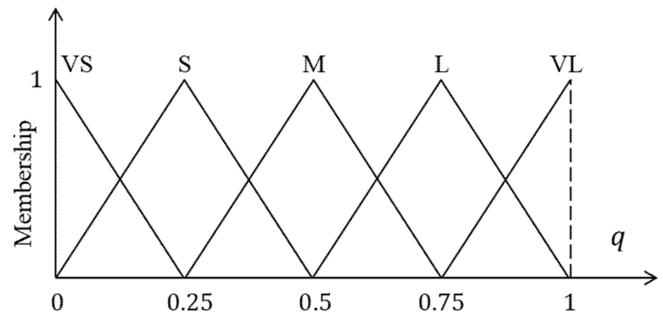
| VS | S | M | L | VL | ||
|---|---|---|---|---|---|---|
| VS | M | VS | VS | VS | VS | |
| S | M | S | S | VS | VS | |
| M | L | M | S | S | VS | |
| L | L | L | M | S | VS | |
| VL | VL | L | M | M | S | |
| Block Names | Encoder Backbones | |||
|---|---|---|---|---|
| ResNet-18 | ResNet-34 | ResNet-50 | ResNet-101 | |
| Conv-1 | ||||
| Conv-2 | ||||
| Conv-3 | ||||
| Conv-4 | ||||
| Conv-5 | ||||
| Models | Backbones | Time (Unit: ms) | Number of Model Parameters | ||
|---|---|---|---|---|---|
| Min. | Max. | Avg. | |||
| Vanilla | VGG16 | 49.5 | 50.4 | 49.7 | 29,306,465 |
| Res-U-Net-18 | ResNet-18 | 41.9 | 42.8 | 42.2 | 25,009,737 |
| Res-U-Net-34 | ResNet-34 | 44.4 | 44.8 | 44.5 | 35,117,897 |
| Res-U-Net-50 | ResNet-50 | 56.1 | 56.7 | 56.4 | 57,677,897 |
| Res-U-Net-101 | ResNet-101 | 63.9 | 64.5 | 64.1 | 76,670,025 |
| Metrics | IoU | Precision | Recall | F1-Score | |
|---|---|---|---|---|---|
| Vicinity | |||||
| 0-pixel | 0.667 | 0.723 | 0.794 | 0.778 | |
| 1-pixel | 0.801 | 0.895 | 0.856 | 0.890 | |
| 2-pixel | 0.814 | 0.944 | 0.883 | 0.898 | |
Publisher’s Note: MDPI stays neutral with regard to jurisdictional claims in published maps and institutional affiliations. |
© 2021 by the authors. Licensee MDPI, Basel, Switzerland. This article is an open access article distributed under the terms and conditions of the Creative Commons Attribution (CC BY) license (https://creativecommons.org/licenses/by/4.0/).
Share and Cite
Chen, H.-C.; Li, Z.-T. Automated Ground Truth Generation for Learning-Based Crack Detection on Concrete Surfaces. Appl. Sci. 2021, 11, 10966. https://doi.org/10.3390/app112210966
Chen H-C, Li Z-T. Automated Ground Truth Generation for Learning-Based Crack Detection on Concrete Surfaces. Applied Sciences. 2021; 11(22):10966. https://doi.org/10.3390/app112210966
Chicago/Turabian StyleChen, Hsiang-Chieh, and Zheng-Ting Li. 2021. "Automated Ground Truth Generation for Learning-Based Crack Detection on Concrete Surfaces" Applied Sciences 11, no. 22: 10966. https://doi.org/10.3390/app112210966
APA StyleChen, H.-C., & Li, Z.-T. (2021). Automated Ground Truth Generation for Learning-Based Crack Detection on Concrete Surfaces. Applied Sciences, 11(22), 10966. https://doi.org/10.3390/app112210966