
A Method for Calculating the Velocity of Corner-to-Corner Rear-End Collisions of Vehicles Based on Collision Deformation Analysis

Abstract
:
1. Introduction
2. Collision Simulation Experiment
2.1. Design of the Experiment
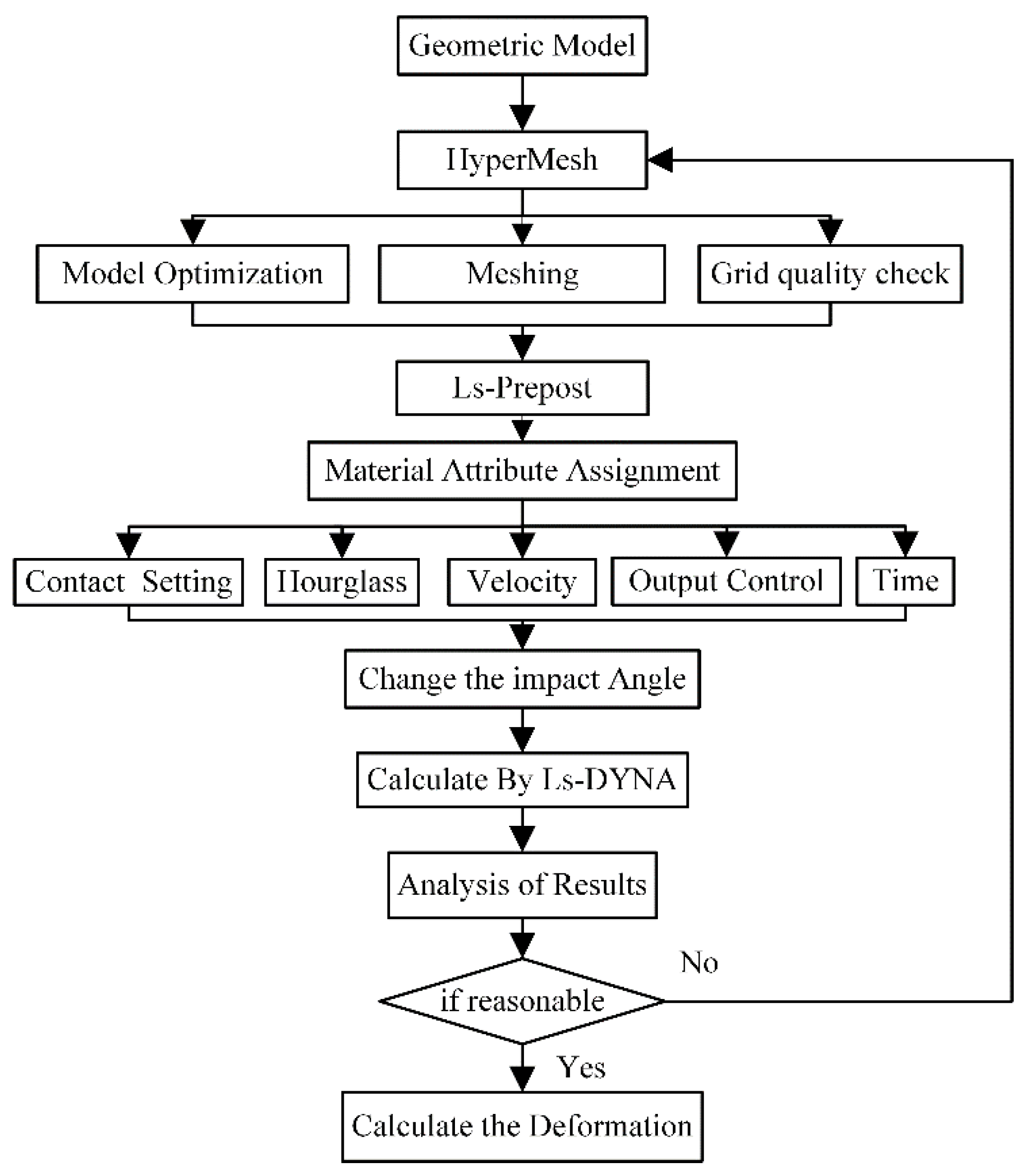
2.2. Finite Element Model of Vehicle
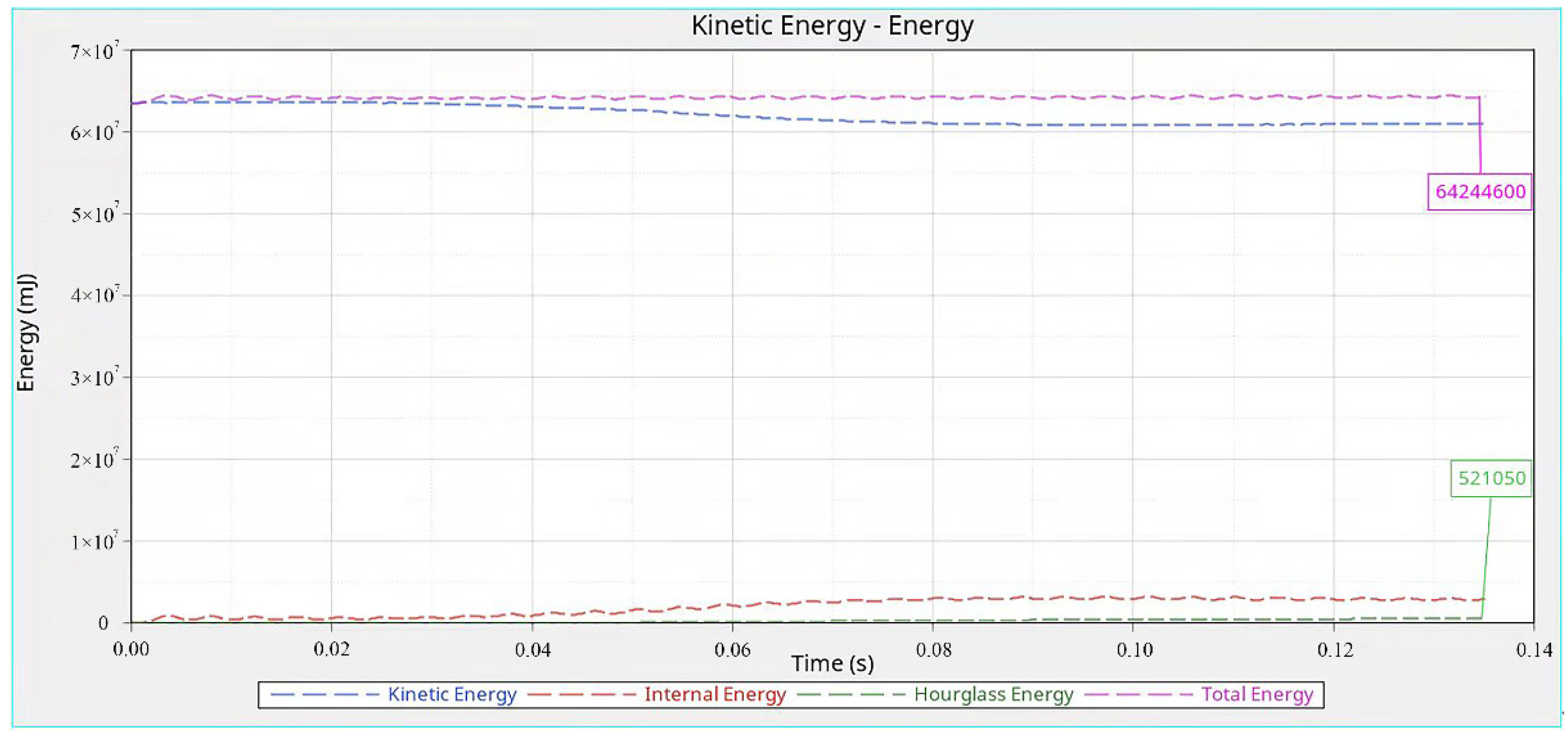
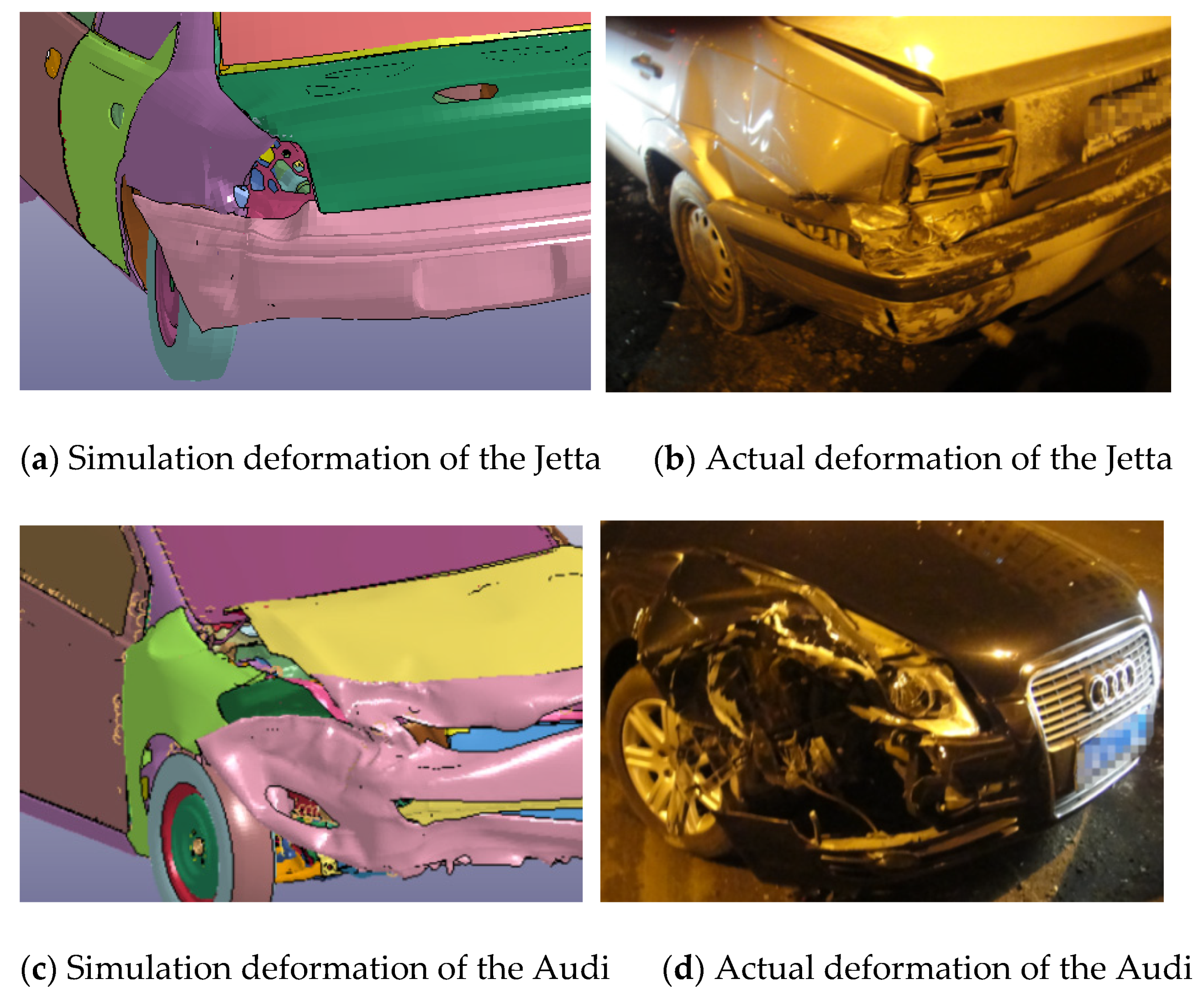
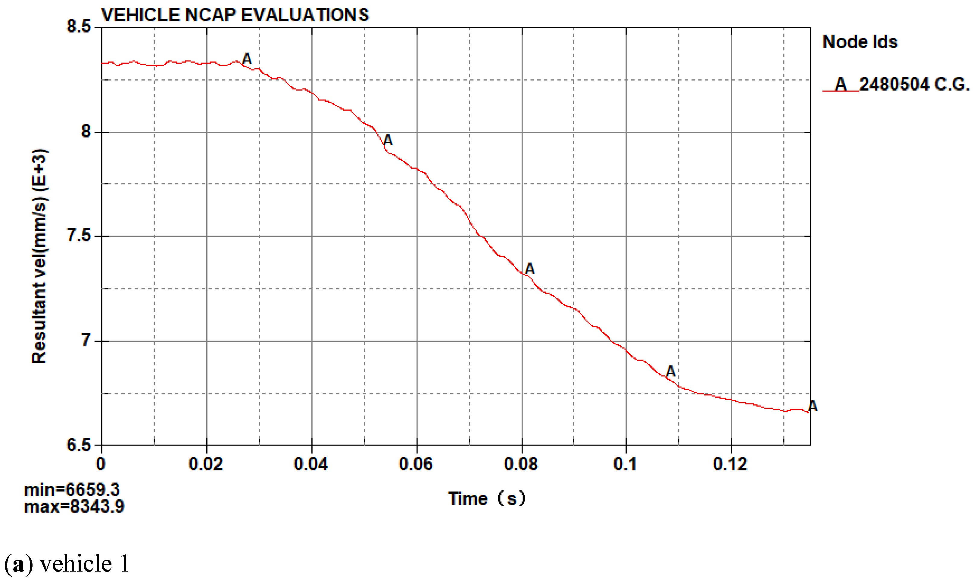
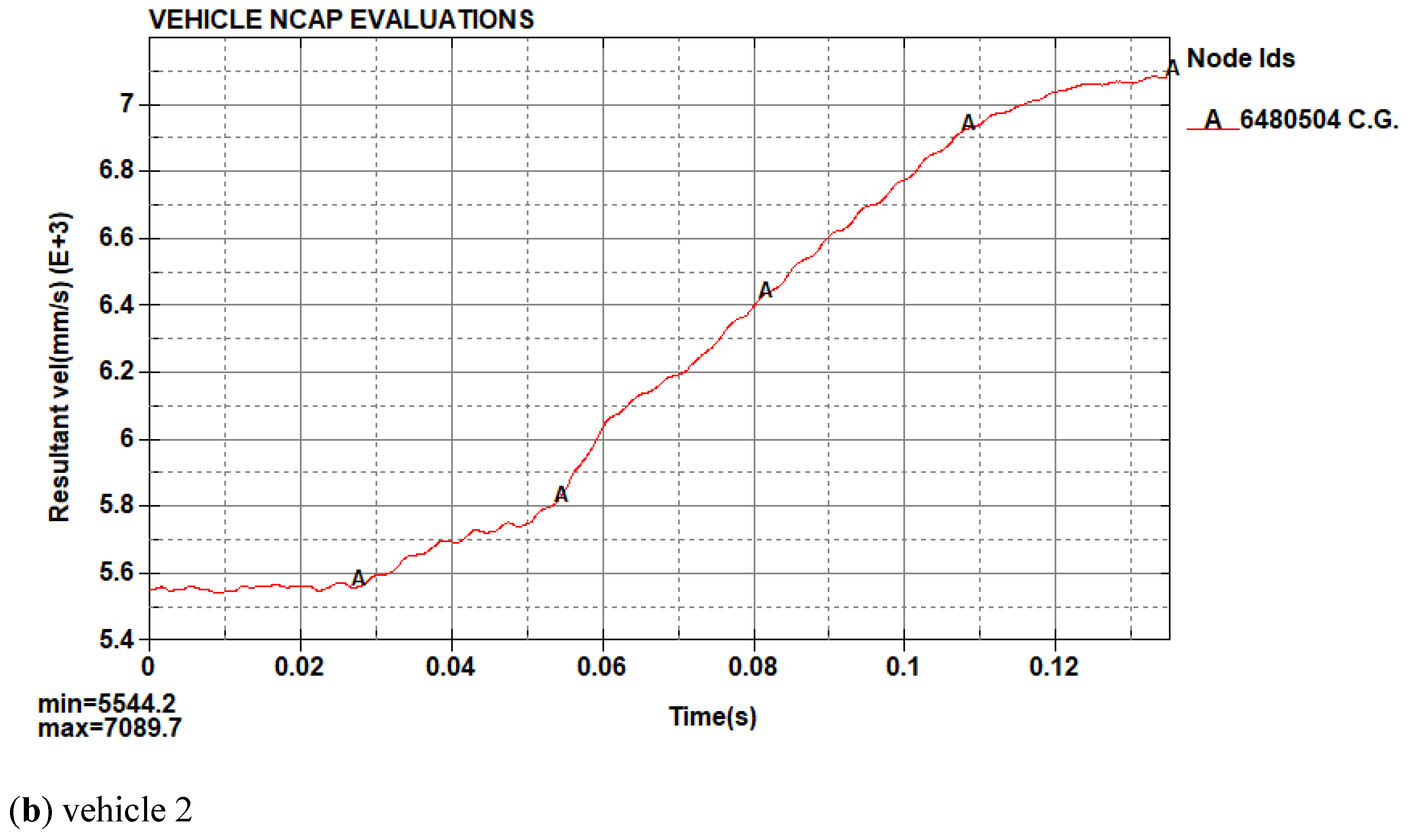
2.3. Model Checking
3. Methodology
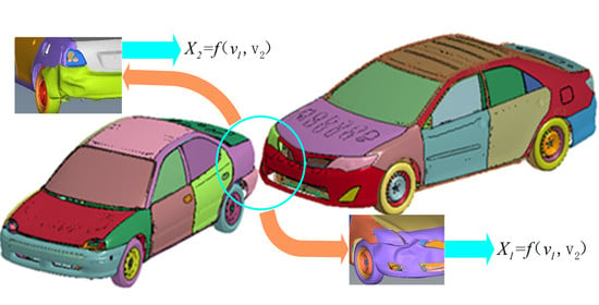
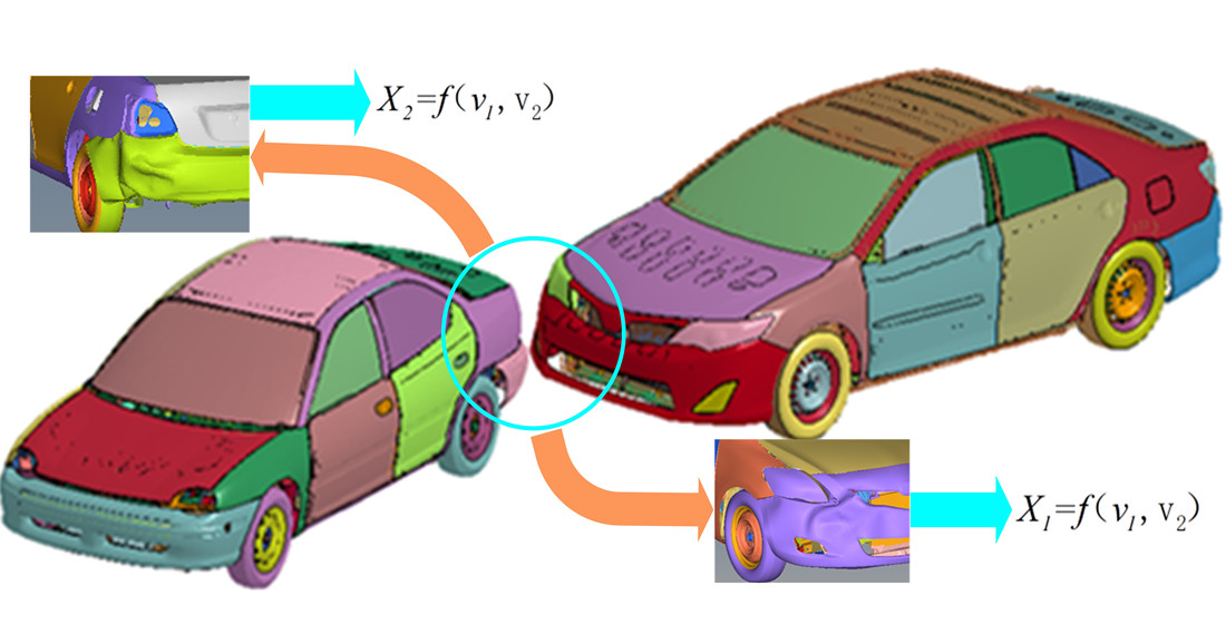
3.1. Calculation Method of Deformation
3.2. Data Collection
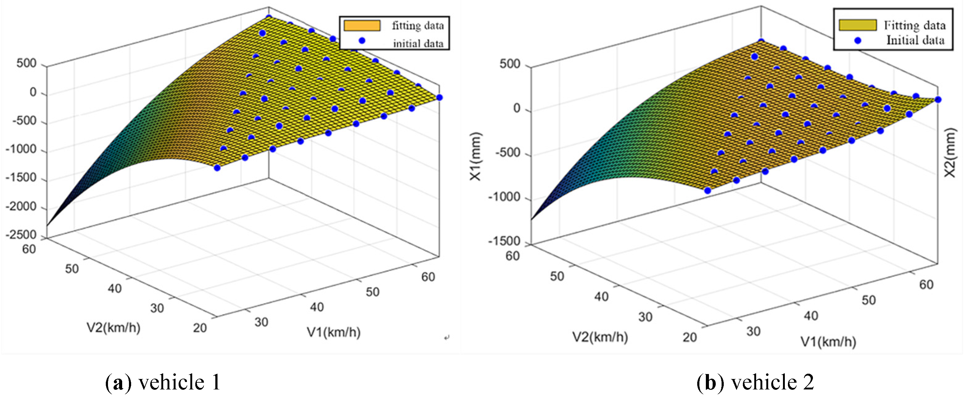
3.3. Data Fitting
4. Case Study
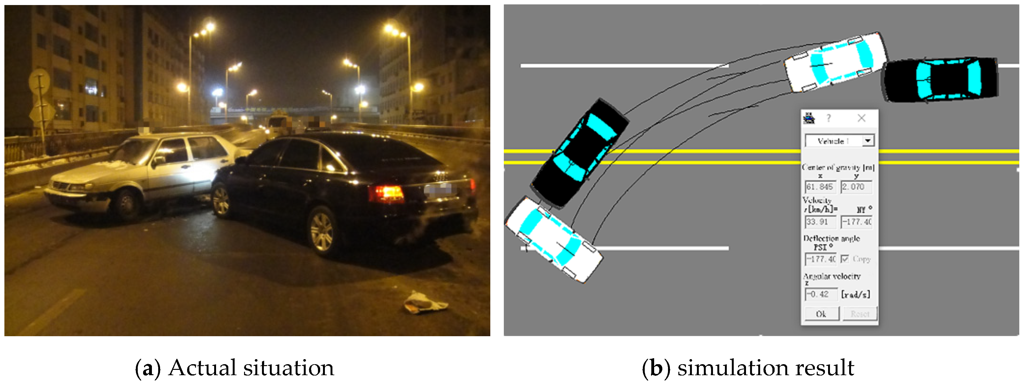
4.1. Brief Case
4.2. Case Solving
4.3. Result Analysis
5. Conclusions
- (1)
- Based on the principles of classical mechanics and the finite element method, a method for solving the velocity of rear-end vehicle collisions is proposed. The case study shows that the results obtained using this method are in good agreement with those calculated with PC-Crash software, and the error is within 5%; reconstruction results of collision deformation are basically consistent with actual deformations, and the error is within 15%.
- (2)
- This method utilizes information from vehicle collision deformations and improves the reliability of analysis results of corner to corner rear-end collision of vehicles. A relationship model between collision velocity and deformation is established that overcomes the limitations of the traditional finite element method, such as low reconstruction efficiency and the model has strong pertinence.
- (3)
- By combining the finite element simulation with the dynamic model method, the vehicle velocity can be quickly calculated according to the vehicle deformation, which breaks through the traditional algorithm of calculating the vehicle velocity using tire traces and scattered objects, and improves the efficiency and accuracy of the calculation results.
Author Contributions
Funding
Institutional Review Board Statement
Informed Consent Statement
Data Availability Statement
Conflicts of Interest
References
- McHenry, B.G.; McHenry, R.R. SMAC-97-Refinement of the Collision Algorithm. SAE Trans. 1997, 106, 1523–1536. [Google Scholar]
- McHenry, B.G.; McHenry, R.R. CRASH-97-Refinement of the Trajectory Solution Procedure. SAE Trans. 1997, 106, 1537–1556. [Google Scholar]
- Steffan, H.; Moser, A. The Collision and Trajectory Models of PC-CRASH; 960886; SAE International: Detroit, MI, USA, 1996. [Google Scholar]
- Zhang, X.; Jin, X. Study of Vehicle Accident Reconstruction Based on the Information of the tire marks. J. Harbin Inst. Technol. 2007, 14, 641–645. [Google Scholar]
- Huang, J.; Jin, X. A Computer Reconstruction Method for Car-to-Car Collisions Traffic Accidents. J. Shanghai Jiaotong Univ. 2005, 39, 1449. [Google Scholar]
- Han, I. Analysis of vehicle collision accidents based on qualitative mechanics. Forensic Sci. Int. 2018, 291, 53–61. [Google Scholar] [CrossRef] [PubMed]
- Zou, T.; Hu, L. A simple algorithm for analyzing uncertainty of accident reconstruction results. Forensic Sci. Int. 2015, 257, 229–235. [Google Scholar] [CrossRef]
- Guo, L.; Jin, X. A Method of Reconstruction of Vehicle Collision Accidents Based on Body Deformation. J. Shanghai Jiaotong Univ. 2008, 8, 1334–1337, 1343. [Google Scholar]
- Zhiqiang, L.; Aihong, Z.; Liang, J. A simplified model for analysis of side-impact velocity based on energy method. In IOP Conference Series: Materials Science and Engineering; IOP Publishing: Bristol, UK, 2018; Volume 392, p. 062126. [Google Scholar]
- Voevodin, E.; Baklanova, K.; Kovalev, V. The Vehicle’s Driving Dynamics Test at the Collision of Vehicles. Transp. Res. Procedia 2021, 54, 672–681. [Google Scholar] [CrossRef]
- Vangi, D. A simplified model for analysis of the post-impact motion of vehicles. Proc. Inst. Mech. Eng. Part D J. Automob. Eng. 2013, 227, 779–788. [Google Scholar] [CrossRef]
- Vangi, D.; Begani, F. Energy loss in vehicle collisions from permanent deformation: An extension of the ‘Triangle Method’. Veh. Syst. Dyn. 2013, 51, 857–876. [Google Scholar] [CrossRef]
- Vangi, D.; Begani, F. Vehicle accident reconstruction by a reduced order impact model. Forensic Sci. Int. 2019, 298, 426.e1–426.e11. [Google Scholar] [CrossRef] [PubMed]
- Ji, A.; Levinson, D. An energy loss-based vehicular injury severity model. Accid. Anal. Prev. 2020, 146, 105730. [Google Scholar] [CrossRef] [PubMed]
- York, A.R.; Day, T.D. The DyMESH method for three-dimensional multi-vehicle collision simulation. SAE Trans. 1999, 108, 365–382. [Google Scholar]
- El-Tawil, S.; Severino, E. Vehicle collision with bridge piers. J. Bridge Eng. 2005, 10, 345–353. [Google Scholar] [CrossRef] [Green Version]
- Fahlstedt, M.; Baeck, K. Influence of impact velocity and angle in a detailed reconstruction of a bicycle accident. In Proceedings of the International Research Council on the Biomechanics of Injury Conference, IRCOBI 2012, Dublin, Ireland, 12–14 September 2012; Volume 40, pp. 787–799. [Google Scholar]
- Macurová, Ľ.; Kohút, P. Determinig the energy equivalent speed by using software based on the finite element method. Transp. Res. Procedia 2020, 44, 219–225. [Google Scholar] [CrossRef]
- Evtiukov, S.; Golov, E. Finite element method for reconstruction of road traffic accidents. Transp. Res. Procedia 2018, 36, 157–165. [Google Scholar] [CrossRef]
- Zhang, X.; Jin, X. Vehicle crash accident reconstruction based on the analysis 3D deformation of the auto-body. Adv. Eng. Softw. 2008, 39, 459–465. [Google Scholar] [CrossRef]
- Chen, Q.; Xie, Y. A deep neural network inverse solution to recover pre-crash impact data of car collisions. Transp. Res. Part C Emerg. Technol. 2021, 126, 103009. [Google Scholar] [CrossRef]
- Yao, G. Application Manual of Automotive Metal Materials; Beijing University of Technology Press: Beijing, China, 2002; pp. 16–18. [Google Scholar]
- Zheng, H.; Lu, Y. FEM Simulation Analysis of Frontal Crashworthiness for a Vehicle. J. Chongqing Univ. Technol. Nat. Sci. 2018, 31–37, 134. [Google Scholar]
- Pei, Y.; Jiang, X. Road Traffic Accident Analysis and Reappearance Technology; Communication Press: Beijing, China, 2010; pp. 117–120. [Google Scholar]


| Number | Parts | Material Number | Density (t/mm³) | Young’s Modulus (Mpa) | Poisson’s Ratio | Yield Stress (Mpa) |
|---|---|---|---|---|---|---|
| 1 | Front fender | 024 | 1.415 × 10⁻⁹ | 1.00 × 10³ | 0.3 | 20 |
| 2 | Bumper | 024 | 7.890 × 10⁻⁹ | 2.00 × 10⁵ | 0.3 | 800 |
| 3 | Door and Hood | 024 | 7.890 × 10⁻⁹ | 2.00 × 10⁵ | 0.3 | 271 |
| 4 | Engine | 001 | 1.582 × 10⁻⁹ | 2.00 × 10⁴ | 0.3 | \ |
| 5 | Engine Cover | 001 | 7.890 × 10⁻⁹ | 2.00 × 10⁵ | 0.3 | \ |
| 6 | Tailgate | 024 | 1.005 × 10⁻⁹ | 1.00 × 10³ | 0.3 | 20 |
| 7 | Roof | 024 | 7.890 × 10⁻⁹ | 2.00 × 10⁵ | 0.3 | 220 |
| 8 | Window Glass | 123 | 2.500 × 10⁻⁹ | 7.00 × 10⁴ | 0.22 | 30 |
| 9 | Tire | 001 | 1.750 × 10⁻⁹ | 3.00 × 10² | 0.3 | \ |
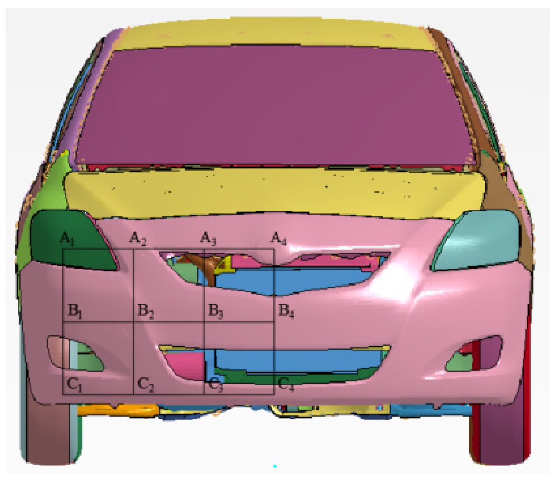
| Key Point | Deformation (mm) | Key Point | Deformation (mm) | ||||
|---|---|---|---|---|---|---|---|
| X | Y | Z | X | Y | Z | ||
| A1 | 4 | −18 | 49 | B3 | 61 | −34 | 39 |
| A2 | 15 | −25 | 49 | B4 | 24 | −24 | 43 |
| A3 | 23 | −27 | 54 | C1 | 19 | −19 | 39 |
| A4 | 11 | −23 | 56 | C2 | 19 | −20 | 41 |
| B1 | 23 | −21 | 41 | C3 | 15 | −19 | 43 |
| B2 | 71 | −37 | 40 | C4 | 10 | −18 | 50 |
| Overall Deformation of the Vehicle 1: C1 | |||||||||||
|---|---|---|---|---|---|---|---|---|---|---|---|
| V | 20 km/h | 25 km/h | 30 km/h | 35 km/h | 40 km/h | 45 km/h | 50 km/h | 55 km/h | 60 km/h | 65 km/h | |
| Overall deformation of the vehicle 2: C2 | 20 km/h | - | 29 | 57 | 70 | 119 | 132 | 155 | 178 | 277 | 354 |
| 25 km/h | 108 | - | 36 | 58 | 88 | 98 | 101 | 123 | 229 | 276 | |
| 30 km/h | 156 | 134 | - | 43 | 69 | 96 | 110 | 116 | 143 | 189 | |
| 35 km/h | 174 | 196 | 150 | - | 53 | 67 | 102 | 103 | 114 | 139 | |
| 40 km/h | 179 | 275 | 217 | 164 | - | 63 | 85 | 108 | 120 | 148 | |
| 45 km/h | 191 | 278 | 255 | 273 | 186 | - | 50 | 101 | 111 | 135 | |
| 50 km/h | 221 | 311 | 294 | 292 | 257 | 182 | - | 71 | 96 | 119 | |
| 55 km/h | 222 | 317 | 320 | 325 | 362 | 285 | 224 | - | 126 | 125 | |
| 60 km/h | 228 | 324 | 346 | 379 | 387 | 388 | 342 | 343 | - | 92 | |
| 65 km/h | 286 | 305 | 365 | 403 | 410 | 452 | 415 | 354 | 306 | - | |
| i | 1 | 2 | 3 | 4 | 5 | 6 | 7 | 8 | 9 |
|---|---|---|---|---|---|---|---|---|---|
| A1i | 0.00967 | −0.01029 | −0.6034 | −0.2137 | −0.02575 | 0.02614 | 19.21 | −17.93 | 0.8444 |
| A2i | 0.00585 | −0.00231 | −0.2844 | −1.818 | −0.02741 | 0.02769 | −5.814 | 14.45 | 1.79 |
| Calculation Results | Method of Calculation | Comparative | |
|---|---|---|---|
| PC-Crash | Mathematical Model Calculation | Relative Error | |
| Driving Velocity: v1 (km/h) | 33.91 | 35.42 | 4.45% |
| Driving Velocity: v2 (km/h) | 33.53 | 32.20 | 3.97% |
Publisher’s Note: MDPI stays neutral with regard to jurisdictional claims in published maps and institutional affiliations. |
© 2021 by the authors. Licensee MDPI, Basel, Switzerland. This article is an open access article distributed under the terms and conditions of the Creative Commons Attribution (CC BY) license (https://creativecommons.org/licenses/by/4.0/).
Share and Cite
Cao, Y.; Ye, X.; Han, G. A Method for Calculating the Velocity of Corner-to-Corner Rear-End Collisions of Vehicles Based on Collision Deformation Analysis. Appl. Sci. 2021, 11, 10964. https://doi.org/10.3390/app112210964
Cao Y, Ye X, Han G. A Method for Calculating the Velocity of Corner-to-Corner Rear-End Collisions of Vehicles Based on Collision Deformation Analysis. Applied Sciences. 2021; 11(22):10964. https://doi.org/10.3390/app112210964
Chicago/Turabian StyleCao, Yi, Xingwang Ye, and Geng Han. 2021. "A Method for Calculating the Velocity of Corner-to-Corner Rear-End Collisions of Vehicles Based on Collision Deformation Analysis" Applied Sciences 11, no. 22: 10964. https://doi.org/10.3390/app112210964
APA StyleCao, Y., Ye, X., & Han, G. (2021). A Method for Calculating the Velocity of Corner-to-Corner Rear-End Collisions of Vehicles Based on Collision Deformation Analysis. Applied Sciences, 11(22), 10964. https://doi.org/10.3390/app112210964