Abstract
This paper addresses the structural-parametric synthesis and kinematic analysis of the RoboMech class of parallel mechanisms (PM) having two sliders. The proposed methods allow the synthesis of a PM with its structure and geometric parameters of the links to obtain the given laws of motions of the input and output links (sliders). The paper outlines a possible application of the proposed approach to design a PM for a cold stamping technological line. The proposed PM is formed by connecting two sliders (input and output objects) using one passive and one negative closing kinematic chain (CKC). The passive CKC does not impose a geometric constraint on the movements of the sliders and the geometric parameters of its links are varied to satisfy the geometric constraint of the negative CKC. The negative CKC imposes one geometric constraint on the movements of the sliders and its geometric parameters are determined on the basis of the Chebyshev and least-square approximations. Problems of positions and analogues of velocities and accelerations of the considered PM are solved to demonstrate the feasibility and effectiveness of the proposed formulations and case of study.
1. Introduction
The design of manipulation robots both with serial and parallel manipulators is carried out mainly by solving inverse kinematics and developing the control systems and technical means according to the obtained laws of motions of the actuators [1,2,3,4]. In this case, the actuators of manipulation robots may work in controlled regimes of intensive accelerations and braking that worsen their dynamics and mechanical efficiency [5,6].
In order to improve the dynamic characteristics and simplify the control systems of the designed manipulators, it is advisable to set the laws of motions of the actuators along with the given laws of the end-effectors’ motions. The ability to set the laws of motions of the input links improves the dynamic parameters and simplifies the control system and therefore also increases the reliability and reduces the cost of the designed manipulator. Such parallel manipulators, having the property of manipulation robots, such as reproducing the given laws of motions of end-effectors, and the property of mechanisms, such as setting the laws of motions of actuators, are called the RoboMech class parallel mechanisms or paralell manipulators (PMs) [7].
In the simultaneous setting the laws of motions of the input and output links, the RoboMech class PMs operate under certain structural schemes and geometric parameters of their links. In this case, the control elements for the movement of the PMs, i.e., the functional relationship between the laws of motions of the input and output links, is laid in the determining structure schemes and geometric parameters of the links, i.e., in the mechanical part of the RoboMech class PMs. Such an optimal combination of mechanics and motion control of manipulation robots corresponds to the modern concept of mechatronics as a methodology for developing of simple, reliable and cheap technological automation.
The base for the structural synthesis of planar mechanisms is proposed by Assur [8], according to whom the mechanism is formed by connecting to the input link (actuator) and the base of structural groups with zero degrees of freedom (DOF). These structural groups are then called the Assur groups, which can be of different classes and orders. The existing methods of structural synthesis of mechanisms and manipulators are devoted to the determination of their structural schemes according to the given numbers of DOFs, links, kinematic pairs and their types [9,10,11,12,13,14,15]. A review of research on the synthesis of types of parallel robotic mechanisms was undertaken in [16]. All of these methods do not take into account the functional purposes of mechanisms or manipulators.
In kinematic synthesis (dimensional or parametric synthesis) of mechanisms, with their known structural schemes, the synthesis parameters are determined by the given positions of the input and output links. Generation of the specified movements of output links (output objects) can be performed exactly and approximately. Exact reproduction of the required movements of a rigid body by linkage mechanisms is possible with a limited number of positions, depending on the structural scheme of the mechanism-generator, while the possibility of their approximate reproduction is not limited to the number of specified positions.
Exact methods for synthesis of mechanisms, or so-called geometric methods, are based on kinematic geometry. The fundamentals of kinematic geometry for finite positions of a rigid body in a plane motion were developed by Burmester and for finite-positions of a rigid body in space were developed by Shoenflies. Burmester in [17] developed the theory of a moving plane having four and five positions on circles. Shoenflies in [18] formulated theorems on the geometrical places of points of a rigid body having seven positions on a circle and three positions on a line. The graphical methods of Burmester and Schoenflies theories received an analytical interpretation [19,20,21], which is summarized in the monograph.
Geometric methods of mechanism synthesis are clear and simple. However, these methods are applicable only for a limited number of positions. Moreover, the algorithms for solving problems using these methods depend significantly on the number of specified positions, and their complexity increases with the number of positions. Approximation (algebraic) methods of mechanism synthesis are devoid of these disadvantages.
Problems of approximation synthesis of mechanisms were first formulated and solved in [22]. Least-square approximations are the most widely used in the approximation synthesis of mechanisms. For the development of this method, a new deviation function, a weighted difference with a parametric weight, proposed in [23], was important. In contrast to the actual deviation, the weighted difference can be reduced to linear forms (generalized polynomials). This makes it quite easy to apply linear approximation methods to the synthesis of mechanisms. This eliminates the limit on the maximum number of specified positions of the moving object.
Combining the main advantages of geometric and approximation methods, a new direction-approximation kinematic geometry of mechanism synthesis was formulated. It studies a special class of approximation problems related to the definition of points and lines of a rigid body describing the constraint of the synthesizing kinematic chains. In the works [24,25], the basics of approximation kinematic geometry of the plane and spatial movements are presented, where circular square points [24] and points with approximately spherical and coplanar trajectories [25] are defined, which correspond to binary links of the type RR, SS and SPk. Further, in the works [26,27], the concept of discrete Chebyshev approximations was introduced for the kinematic synthesis of linkage mechanisms. Theorems characterizing the Chebyshev circle and straight line in plane motion [26] and the Chebyshev sphere and plane in spatial motion [27], as well as iterative algorithms for determining Chebyshev circular, spherical and other points based on minimizing the limit values of the weighted difference, are formulated.
Many approaches for kinematic analysis and synthesis of mechanisms and manipulators are based on the derivative of loop-closure equations using the vector, matrix and screw methods [28,29,30,31,32,33,34,35,36,37,38,39,40,41,42]. In this case, polynomials of high degrees are obtained [43,44].
In this paper, structural-parametric synthesis and kinematic analysis of the RoboMech class PM with two sliders is carried out on the base of modular approach, according to which, by the given laws of motions of the input and output links, the structural scheme and geometric parameters of links are determined from the separate simple structural modules [45]. The considered PM is formed by connecting two sliders using one passive and one negative closing kinematic chain (structural (modules) having zero and negative DOF, respectively. This PM can be used in a cold stamping technological—line as proposed in a case of study.
2. Structural Scheme of a Cold Stamping Technological Line
A scheme of a simple single-stream robotic cold stamping technological line [46] is shown in Figure 1, where TE is the main technological equipment, IR is an industrial robot and S is a piece-by-piece delivery store.
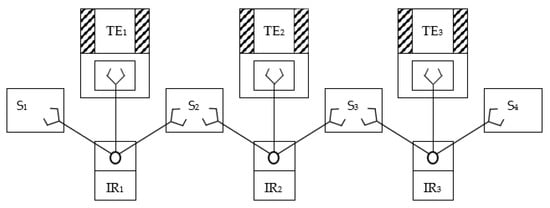
Figure 1.
Scheme of a single-stream robotic cold stamping technological line.
This scheme is typical for technological processes with a small cycle of processing production items on technological equipment, in particular, in cold stamping process. In this scheme, there is no inter-operational transport system, and products (production items) are transferred from one piece of technological equipment to another directly by industrial robots.
The equipment of the presented scheme of the technological line operate in the following sequence: the first industrial robot IR1 takes a workpiece in a certain position from the first store S1 and delivers it to the first piece of technological equipment TE1, where the workpiece is processed (stamped). After primary processing, the product is delivered by the same industrial robot IR1 to the second store S2, where the position of the product is changed for sequent processing. Then, the second industrial robot IR2 delivers the product from the store S2 to the second piece of technological equipment TE2, where the second processing of the product is carried out. After this processing, the product is delivered to the store S3 by the second industrial robot IR2. Moreover, all equipment must operate in accordance with a given cyclogram of the technological line.
Thus, the considered technological line for processing the product with two changing positions of the product has two main pieces of technological equipment (hydraulic presses), I and II, four auxiliary pieces of equipment: a device III for feeding the workpiece, a device IV for removing the product after processing and two industrial robots V and VI (Figure 2). These devices in total have of eight DOF. It is known that the more DOF of equipment in technological lines for mass production of typical products, the lower their productivity and reliability.
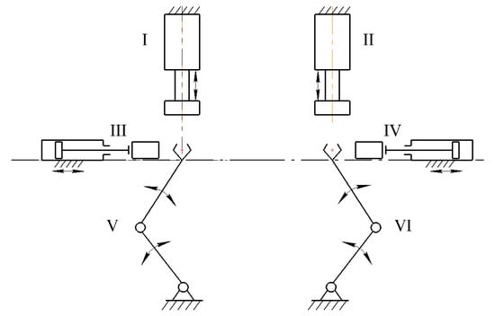
Figure 2.
Scheme of the technological line with eight DOFs.
In order to eliminate the noted disadvantages of the technological line, we reduce its number of DOF, replacing the technological and auxiliary equipment with the RoboMech class PMs. According to the developed principle of forming the RoboMech class PMs [7], we combine the main technological equipment (hydraulic presses) I and II with devices for feeding the workpieces III and removing the workpieces IV, and also combine two industrial robots V and VI into one PM with two end-effectors.
Combination of the hydraulic presses I and II with the devices for feeding the workpieces III and removing the workpieces IV into PMs I’ and II’ with two sliders is carried out by connecting the punches Q’ and Q’’ of the hydraulic cylinders I and II with the sliders P’ and P’’ of the workpieces feeding and removing devices III and IV using passive CKCs A’B’C’ and A’’B’’C’’, as well as negative CKCs D’E’ and D’’E’’, respectively (Figure 3).
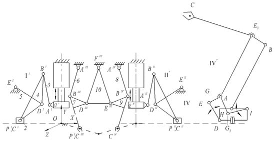
Figure 3.
Structural scheme of the technological line with the RoboMech class PMs.
Combination of two industrial robots (serial manipulators) AIIIBIIICIII and AIVBIVCIV into one PM III′ with two output points is carried out by connecting the links BIIICIII and BIVCIV of the serial manipulators AIIIBIIICIII and AIV BIVCIV using negative CKC DIIIEIIIFIII.
As a result, we obtain a scheme of a technological line with the RoboMech class PMs with three DOFs, where the presses I’ and II’ have two DOF, the PM with two output point III’ have one DOFs. Hydraulic presses I’ and II’ with devices for feeding and removing workpieces work in the OXY plane, and the PM with two output points III’ works in the OXZ plane. Figure 3 also shows a scheme of the PM IV′ operating in a cylindrical coordinate system. This PM is used to store finished products in bins.
The considered technological line with the RoboMech class PMs operates as follows. When feeding the workpiece for processing by the press I’, the slider P’ takes the right extreme position, and the punch Q’ of the hydraulic cylinder takes the upper extreme position. When processing the workpiece, the punch Q’ of this press takes the lower extreme position, and the slider P’ returns to the left extreme position to deliver the next workpiece. At the moment of return of the punch Q’ of the hydraulic cylinder I’ to the upper position, the first gripper C’’’ of the PM with two output points takes the extreme left position, captures the processed workpiece and delivers it to the store. At this moment, the second gripper CIV delivers the previously processed workpiece to the press II′ for further processing, i.e., takes the extreme upper position. After the secondary processing of the workpiece, the finished product is delivered to the container by the slider P’’. Then the cycle is repeated.
After accumulation of products in the container, it is stored in bins with the help of PM IV’. A gripper CV of this PM reproduces the series of horizontal and vertical trajectories. In this case, the series of horizontal trajectories are reproduced by input link DVEV and the series of vertical trajectories are reproduced by input link IVHV drive. Rotation of the entire PM around the vertical axis provides a spatial movement of the gripper CV in a cylindrical coordinate system. Structural-parametric synthesis of this PM is considered in [47]. Let us consider the structural-parametric synthesis of the PM with two sliders.
3. Structural-Parametric Synthesis of the PM with Two Sliders
The problem of structural-parametric synthesis of the PM with two sliders is to determine the structural scheme and geometric parameters of links, when the first slider Q (the punch of a hydraulic press) takes the lower extreme position with a stroke , the second slider P takes the left extreme position with a stroke (Figure 4a) and also, when the first slider Q takes the upper extreme position with a stroke , and the second slider P takes the right extreme position with a stroke (Figure 4b). For the convenience of reporting the strokes of the sliders, the absolute coordinate system OXY is located at the point of their intersection.
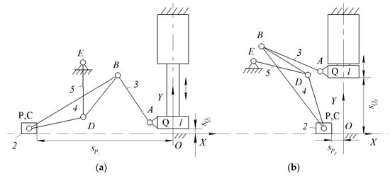
Figure 4.
(a) lower extreme and (b) upper extreme positions of the slider Q.
As noted above, to form the PM with two sliders, providing their specified positions, we connect the punch Q of the hydraulic press and the slider P using the dyad ABC with revolute kinematic pairs. The dyad ABC has zero DOF and it is a passive CKC, which does not impose geometric constraints on the movements of the punch Q and the slider P. Therefore, the passive CKC ABC allows reproduction of the specified movements of the sliders Q and P. Then we connect the link BC of the dyad ABC with a base using a binary link DE with revolute kinematic pairs, which has one negative DOF, it is a negative CKC. Negative CKC DE imposes one geometric constraint on the movements of the sliders Q and P, and as a result, we obtain a structural scheme of the PM with structural formula I (0,1) → III (3,4,2,5), where the kinematic chain 3-4-2-5 represents the Assur group of the third class [48]. Figure 5 shows a block structure of the formed PM with two sliders.
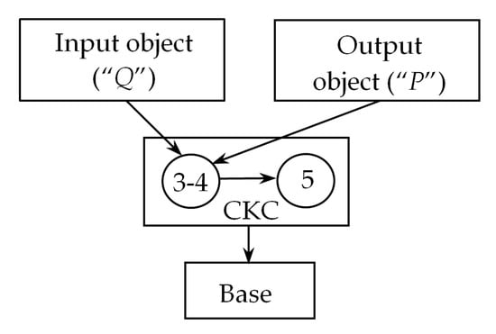
Figure 5.
Block structure of the PM with two sliders.
For parametric synthesis of the PM with two sliders, let us consider its i-th intermediate position and attach the coordinate systems and with the sliders (Figure 6), the axes and which are directed parallel to the axis OX of the absolute coordinate system OXY. Then, the movements of the sliders are determined by the parameters and of the coordinate systems and Qx2y2 movements, where i = 1, 2 ..., N (N is the number of given positions). Parametric synthesis of this PM with two sliders, according to its block structure (Figure 5), consists of a parametric synthesis of the passive CKC ABC and the negative CKC DE.
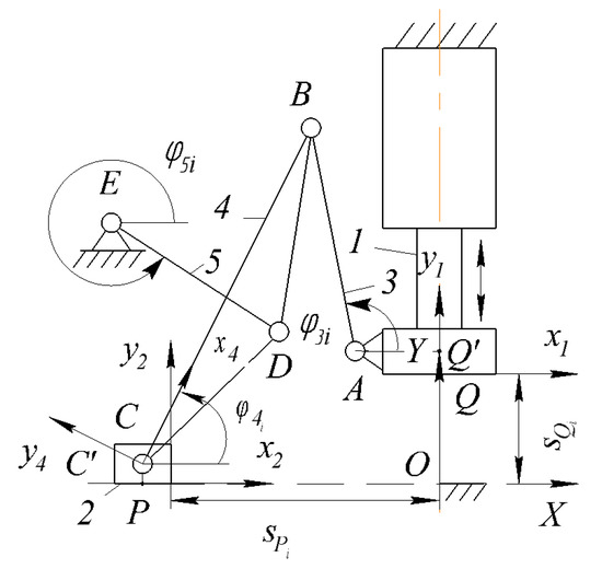
Figure 6.
Intermediate position of the PM with two sliders.
The synthesis parameters (geometric parameters of the links) of the passive CKC ABC is a vector where and are the coordinates of the joints A and C in the moving coordinate systems and respectively, and are the lengths of the links AB and BC. Since the passive CKC ABC does not impose geometric constraint on the movements of the sliders Q and P, then its synthesis parameters are set, they are varied by the generator of sequence [49] depending on the geometric constraint imposed by the negative CKC DE. Negative CKC DE imposes one geometric constraint on the movements of the links AB and BC of the passive CKC ABC; therefore, its synthesis parameters are determined.
Let us consider the parametric synthesis of the negative CKC DE. To do this, it is necessary to first determine the angle φ4i by the expression
where
Coordinates and of the joints A and C in the absolute coordinate system OXY in Equations (2) and (3) are determined by the expressions
With the link CB of the dyad ABC, we attach the coordinate system , the axis of which is directed along the link CB. Then, the synthesis parameters of the negative CKC DE are the vector where and are the coordinates of the joints E and D in the coordinate systems and OXY, respectively.
Let us consider the motion of the plane in the absolute coordinate system OXY. In this case, the joint moves along an arc of a circle with a center at the joint and a radius . Consequently, an equation of the geometric constraint imposed by the negative CKC DE of the RR type on the motion of the moving plane is expressed as a weighted difference
where and are the coordinates of the joint E in the absolute coordinate system OXY, which are determined by the expression
After substituting Equation (6) into Equation (5) and replacing the synthesis parameters of the form
then Equation (5) is expressed linearly in two groups of synthesis parameters and in the form
where and are the coefficients of the vectors and free terms depending on the remaining synthesis parameters, which have the form
where is a rotation matrix of view
The linear representability of Equation (5) allows one to formulate and solve the Chebyshev and least-square approximations for parametric synthesis [50]. In the Chebyshev approximation problem, the vectors of synthesis parameters are determined from the minimum of the functional
In the least-square approximation problem, the synthesis parameters vectors are determined from the minimum of the functional
The linear representability of Equation (5) allows the use of the kinematic inversion method, which is an iterative process, at each step of which one group of synthesis parameters is determined to solve the Chebyshev approximation problem (Equation (14)). In this case, the linear programming problem is solved [51]. To do this, we introduce a new variable where is the required approximation accuracy. Then the minimax problem (Equation (14)) leads to the following linear programming problem: determine the minimum of the sum
with the following constraints
where
The sequence of the obtained values of the function will decrease and have a limit as a sequence bounded below, because for any
Let consider the least-square approximation problem (Equation (15)) for the synthesis. The necessary conditions for the minimum of functions (Equation (15)) with respect to the parameters
leading to the systems of linear equations
where
Solving these systems of linear equations for each group of synthesis parameters for given values of the remaining groups of synthesis parameters, we determine their values
at . If , then the revolute kinematic pair is replaced by prismatic kinematic pair.
The matrix can be represented as a product , where is a matrix with dimension (in the considered case )
According to the Binet-Cauchy formula [52], the determinant becomes into the sum of the squares of all minors of order r (we assume that ) in the matrix , compiled in ascending order of the column indices, i.e.,
Consequently, the determinant is positive definite together with the principal minors and the solution of the set of linear Equation (21) corresponds to the minimum of the function S with respect to the parameters . Hence, the least-square approximation problem (Equation (15)) can be solved by the linear iterations method, at each step of which one group of parameters is determined. The sequence of values of the function S will be decreasing and have a limit as a sequence bounded below.
4. Kinematic Analysis of the PM with Two Sliders
Given the synthesis parameters and the positions of the hydraulic cylinder punch Q, it is necessary to find the kinematic parameters of the slider P.
This PM (Figure 6) has the structural formula
i.e., the PM contains an Assur group of the third class with one external prismatic kinematic pair [41]. In the literature, there is no solution of kinematics of this type group.
4.1. Position Analysis
For position analysis of the considered PM, we use the method of conditional generalized coordinates [50]. According to this method, we remove the link 5 by disconnecting the elements of the joints D and E and select the slider P as a conditional input link due to the additional DOF that appears. Then, this PM of the third class is transformed into a mechanism of the second class with the structural formula
Derive the function
where is a variable distance between the centers of the disconnected joints D and E, which is determined by the expression
Coordinates and of the joint D center in Equation (30) are determined by the equation
where
To determine the angle in Equation (31), we derive a vector ABC loop-closure equation
In Equation (33) denotes the unit vector.
We transfer to the right side of Equation (33) and square both sides. As a result, we obtain
Next, we define
Thus, Equation (29) is a function of one variable: the conditional generalized coordinate , for the given values of the real generalized coordinate . Minimizing Equation (29) with respect to a variable by the bisection method [53], we determine its values for given values . In this case, the angles and are simultaneously determined. The angle is determined by the expression
4.2. Analogues of Velocities and Accelerations
To solve the problems of analogues of velocities and accelerations of the PM with two sliders, we select its independent vector contours, the number of which is equal to half the number of links of the Assur group, i.e., it is equal to two. As independent vector contours, we choose the contours OQ’ABCC’O and OQ’ABDEO, the vector loop-closure equations of which have the forms
Project the system of Equation (41) on the axes OX and OY of the absolute coordinate system OXY
Differentiate the system of Equation (42) with respect to the generalized coordinate
From the system of Equation (43) we determine the analogues of velocities
where
Differentiate the system of Equation (43) with respect to the generalized coordinate
Then we obtain the analogues of accelerations
where
5. Numerical Results and Prototyping
N = 11 positions and of the input and output sliders of the PM with two sliders are shown in Table 1.

Table 1.
Positions of the input and output sliders.
Table 2 and Table 3 show the obtained values of the synthesis parameters of the passive CKC ABC and negative CKC DE, respectively.
Table 2.
Synthesis parameters of the passive CKC ABC.
Table 3.
Synthesis parameters of the negative CKC DE.
3D CAD model of the synthesised PM with two sliders is shown in Figure 7.
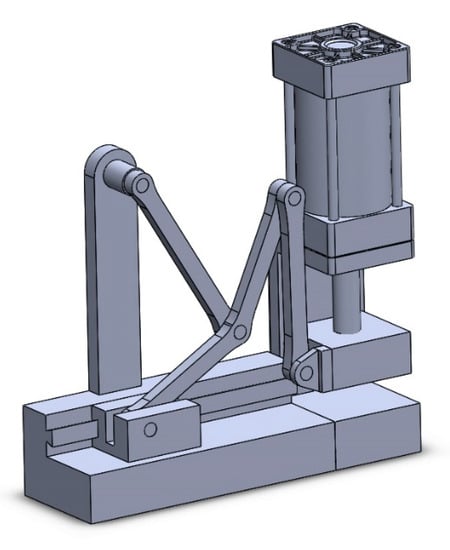
Figure 7.
3D CAD model of the PM with two sliders.
Table 4 shows the obtained values of the positions and analogues of the linear velocities and linear accelerations of the output slider P.
Table 4.
Positions and anologues of the linear velocities and accelerations of the output slider P.
Graphics of the parameters , , are shown in Figure 8.
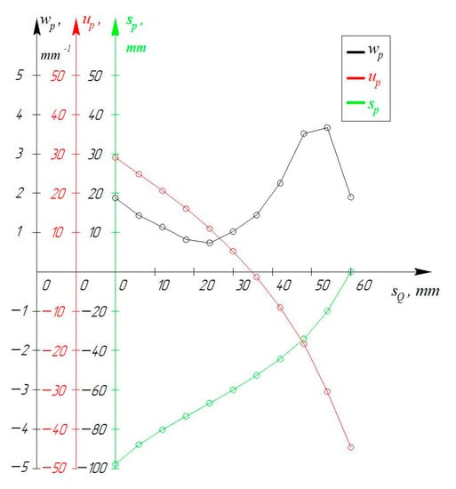
Figure 8.
Graphics of the parameters ,,.
A prototype of the PM with two sliders, and a block scheme of its characteristics are shown in Figure 9 and Figure 10, respectively.
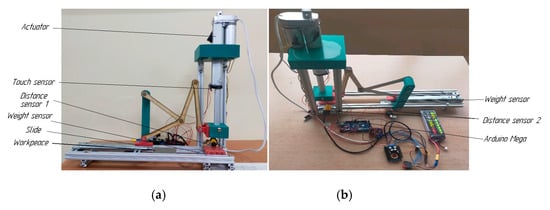
Figure 9.
Prototype of the PM with two sliders: (a) the first position (b) the second position.
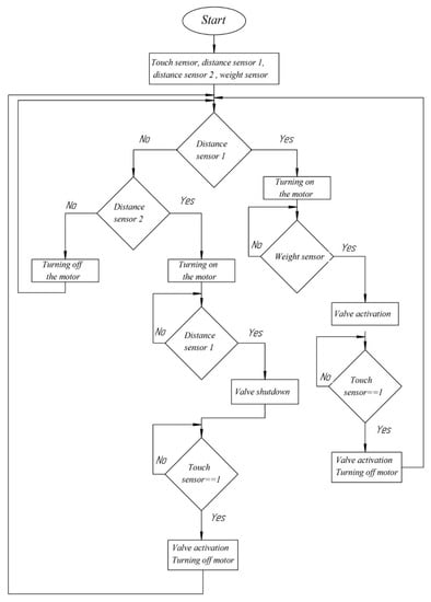
Figure 10.
Block scheme of the PM with two sliders work.
At the beginning, the hydraulic cylinder punch is located at the upper extreme position, and the distance sensor 1 checks a presence of the workpiece for stamping in the die. If there is no workpiece, then the presence of the workpiece in the store is checked using the distance sensor 2. If there is no workpiece in the store, the motor does not turn on. If there is the workpiece in the store, the motor turns on and the punch moves to the lower working position. At this time, the PM slider moves to the left extreme position for the next workpiece.
The first stroke of the punch will be idle. After reaching the lower extreme position of the punch, the distance sensor 1 gives the command to the hydraulic cylinder valve to switch and the punch rises until reaching the touch sensor. In this case, the hydraulic cylinder valve switches, the hydraulic cylinder motor is turned off, and the PM delivers the workpiece to the die (working area). Further, the distance sensor 1 checks the presence of the workpiece in the die.
After delivering the workpiece to the die, the motor turns on and the punch goes down to the lower working position, where the weight sensor is located, which regulates the press force for high-quality stamping. The hydraulic cylinder valve switches after punching, and the punch rises until it reaches the touch sensor. In this case, the hydraulic cylinder valve is switched and its motor is turned off. This cycle is repeated until the end of the workpieces in the store. The connection scheme of the sensors and motor is shown in Figure 11.
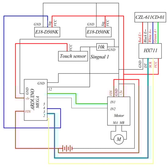
Figure 11.
Connection scheme of the sensors and motor.
6. Conclusions
The scheme of a cold-stamping technological line with the use of RoboMech class PMs has been developed. This technological line uses three RoboMech class PMs: a PM with two sliders, a PM with two end-effectors, and a PM working in a cylindrical coordinate system. The PM with two sliders is formed by connecting two sliders (input and output objects) and a base using one passive and one negative CKC. The formed PM with two sliders contains an Assur group of the third class with one external prismatic kinematic pair. Geometric parameters of the negative CKC are determined on the basis of the Chebyshev and least-square approximations. The problem of the positions of the PM with two sliders is solved using the method of conditional generalized coordinates. The 3D CAD model and prototype of the PM with two sliders have been made.
Author Contributions
Z.B., M.A.L., G.C. developed methods of parametric synthesis and kinematic analysis, A.M., B.A., Y.Z. performed numerical calculations and prototyping of the RoboMech class PM with two sliders. All authors have read and agreed to the published version of the manuscript.
Funding
This research is funded by the Science Committee of the Ministry of Education and Science of Kazakhstan (Grant No AP08857522).
Institutional Review Board Statement
Not applicable.
Informed Consent Statement
Not applicable.
Data Availability Statement
The data presented in the study are available on request from the corresponding author.
Conflicts of Interest
The authors no conflict of interest.
References
- Fu, K.S.; Gonzalez, Z.C.; Lee, C.S.G. Robotics: Control, Sensing, Vision and Intelligence; McGraw–Hill Book Company: London, UK, 1987. [Google Scholar]
- Yoshikava, T. Foundation of Robotics: Analysis and Control; MIT Press: Cambridge, MA, USA, 1990. [Google Scholar]
- Gupta, K.C. Mechanics and Control of Robots; Springer: New York, NY, USA, 1997. [Google Scholar]
- Spong, M.W.; Hutchinson, S.; Vidyasagar, M. Robot Modeling and Control; Hobekon, N.J., Ed.; John Wiley & Sons, Inc.: Hoboken, NJ, USA, 2006. [Google Scholar]
- Song, S.M.; Lee, J.K.; Waldron, K.J. Motion Study of Two—and Three–Dimensional Panthograph Mechanisms. Mech. Mach. Theory 1987, 22, 321–331. [Google Scholar] [CrossRef]
- Waldron, K.J.; Kinzel, G.L. The Relation between Actuator Geometry and Mechanical Efficiency in Robots. In Proceedings of the 4th CISM–IFToMM Symposium on Theory and Practices of Manipulators, Zaborow, Poland, 8–12 September 1981; pp. 366–374. [Google Scholar]
- Baigunchekov, Z.; Kalimoldayev, M.; Ibrayev, S.; Izmambetov, M.; Baigunchekov, T.; Naurushev, B.; Aisa, N. Parallel Manipulator of a Class RoboMech. Lect. Notes Electr. Eng. 2017, 408, 547–557. [Google Scholar]
- Assur, L.V. Investigation of plane hinged mechanism with lower pairs from the point of view of their structure and classification (in Russian). Bull. Petrograd Polytech. Inst. 1914, 21, 187–283. [Google Scholar]
- Hunt, K.H. Kinematic Geometry of Mechanisms; Clarendon Press: Oxford, UK, 1998. [Google Scholar]
- Kong, X.; Gosselin, C.M. Type Synthesis of Parallel Mechanisms; Springer: Berlin/Heidelberg, Germany, 2007. [Google Scholar]
- Sunkari, R.P.; Schmidt, L.C. Structural Synthesis of Planar Kinematic Chains by Adapting McKay–Type Algorithm. Mech. Mach. Theory 2006, 41, 1021–1030. [Google Scholar] [CrossRef]
- Gogu, G. Structural Synthesis of Parallel Robots. Part 3: Topologies with Planar Motion of the Moving Platform; Springer: Dordrecht, The Netherlands, 2010. [Google Scholar]
- Notash, L.; Zhang, J. Structural Synthesis of Kinematic Chains and Mechanisms. Integrated Design and Manufacturing in Mechanical Engineering; Springer: Dordrecht, The Netherlands, 2002; pp. 391–398. [Google Scholar]
- Huang, P.; Ding, H. Structural Synthesis of Assur Groups with up to 12 Links and Creation of Their Classified Databases. Mech. Mach. Theory 2020, 145, 103668. [Google Scholar] [CrossRef]
- Liu, Y.; Li, Y.; Yao, Y.A.; Kong, X. Type Synthesis of Multi-mode Mobile Parallel Mechanisms Based on Refined Virtual Chain Approach. Mech. Mach. Theory 2020, 152, 103908. [Google Scholar] [CrossRef]
- Meng, X.; Gao, F.; Wu, S.; Ge, Q.J. Type synthesis of Parallel Robotic Mechanisms: Framwork and Brief Review. Mech. Mach. Theory 2014, 78, 177–186. [Google Scholar] [CrossRef]
- Burmester, L. Lehrbuch der Kinematik; A. Felix Verlag: Leipzig, Germany, 1988. [Google Scholar]
- Schoenflies, A. Geometric der Bewegung in Synthetischer Darstellung; BG Teubner: Leipzig, Germany, 1886. [Google Scholar]
- Bottema, O.; Roth, B. Theoretical Kinematics; North-Holland Publishing Company: Amsterdam, The Netherlands, 1979. [Google Scholar]
- Bai, S.; Li, Z.; Li, R. Exact Synthesis and Input–Output Analysis of 1-DOF Planar Linkages for Visiting 10 Poses. Mech. Mach. Theory 2020, 143, 103625. [Google Scholar] [CrossRef]
- Hamida, I.B.; Laribi, M.A.; Mlika, A.; Romdhane, L.; Zeghloul, S. Dimensional Synthesis and Performance Evaluation of Four Translational Parallel Manipulators. Robotica 2021, 39, 233–249. [Google Scholar] [CrossRef]
- Chebyshev, P.L. Sur Les Parallélogrammes Composés de Trois Éléments Quelconques. Mémoires l’Académie Sci. St.-Pétersbourg 1879, 36, 1–16. [Google Scholar]
- Levitskii, N.I. Design of Plane Mechanisms with Lower Pairs; Izd. Akad. Nauk USSR: Moscow/Leningrad, Russia, 1950. [Google Scholar]
- Sarkissyan, Y.L.; Gupta, K.C.; Roth, B. Kinematic Geometry Associated with the Least-Square Approximation of a Given Motion. Trans. ASME Ser. B 1973, 95, 503–510. [Google Scholar] [CrossRef]
- Sarkissyan, Y.L.; Gupta, K.C.; Roth, B. Spatial Least-Square Approximation of a Motion. In Proceedings of the IFToMM International Symposium on Linkages and Computer Design Methods, Bucharest, Romania, 7–13 June 1973. [Google Scholar]
- Sarkissyan, Y.L.; Gupta, K.C.; Roth, B. Chebyshev Approximations of Finite Point Sets with Application to Planar Kinematic Synthesis. Trans. ASME J. Mech. Des. 1979, 101, 32–40. [Google Scholar]
- Sarkissyan, Y.L.; Gupta, K.C.; Roth, B. Chebyshev Approximations of Spatial Point Sets Using Spheres and Planes. Trans. ASME J. Mech. Des. 1979, 101, 499–503. [Google Scholar]
- Paul, B. Kinematics and Dynamics of Planar Machinery; Prentice-Hall: Upper Saddle River, NJ, USA, 1979. [Google Scholar]
- Hartenberg, R.S.; Denavit, J. Kinematic Synthesis of Linkages; McGraw-Hill: New York, NY, USA, 1964. [Google Scholar]
- Rodhavan, M.; Roth, B. Solving Polynomial Systems for the Kinematic Analysis and Synthesis of Mechanisms and Robot Manipulators. J. Mech. Des. 1995, 117, 71–79. [Google Scholar]
- Erdman, A.G.; Sandor, G.N.; Kota, S. Mechanism Design: Analysis and Synthesis Lecture Notes; McGill University: Montreal, QC, Canada, 2001. [Google Scholar]
- Uicker, J.J.; Pennack, G.R.; Shigley, J.E. Theory of Machines and Mechanisms, 4th ed.; Oxford University Press: New York, NY, USA, 2001. [Google Scholar]
- Hernandez, A.; Petya, V. Position Analysis of Planar Mechanisms with R-pairs Using Geometrical-Iterative Method. Mech. Mach. Theory 2004, 39, 50–61. [Google Scholar] [CrossRef]
- Pennock, G.R.; Israr, A. Kinematic Analysis and Synthesis of an Adjustable Six-Bar Linkage. Mech. Mach. Theory 2009, 44, 306–323. [Google Scholar] [CrossRef]
- McCarthy, J.M.; Soh, G.M. Geometric Design of Linkages, 2nd ed.; Springer Science & Business Media: Berlin/Heidelberg, Germany, 2010. [Google Scholar]
- Angeles, J.; Bai, S. Kinematic Synthesis, Lecture Notes; McGill University: Montreal, QC, Canada, 2016. [Google Scholar]
- Arikawa, K. Kinematic Analysis of Mechanisms Based on Parametric Polynomial System: Basic Concept of a Method Using Gröbner Cover and Its Application to Planar Mechanisms. J. Mech. Robot. 2019, 11, 020906. [Google Scholar] [CrossRef]
- Baskar, A.; Plecnik, M. Synthesis of Watt-Type Timed Curve Generators and Selection from Continuous Cognate Spaces. J. Mech. Robot. 2021, 13, 051003. [Google Scholar] [CrossRef]
- Fomin, A.; Antonov, A.; Glazunov, V.; Carbone, G. Dimensional (Parametric) Synthesis of the Hexapod-Type Parallel Mechanism with Reconfigurable Design. Machines 2021, 9, 117. [Google Scholar] [CrossRef]
- Duffy, J. Analysis of Mechanisms and Robot Manipulator; Edward Arnold: London, UK, 1980. [Google Scholar]
- Tsai, L.W. Robot Analysis: The Mechanics of Serial and Parallel Manipulators; John Wiley and Sons, Inc.: New York, NY, USA, 1999. [Google Scholar]
- Glazunov, V. Design of Decoupled Parallel Manipulators by Means of the Theory of Screws. Mech. Mach. Theory 2010, 45, 209–230. [Google Scholar] [CrossRef]
- McCarthy, J.M. Kinematics, Polynomials, and Computers-A Brief History. J. Mech. Robot. 2011, 3, 010201–010203. [Google Scholar] [CrossRef] [Green Version]
- McCarthy, J.M. 21st Kinematics Synthesis, Compliance, and Tensegrity. J. Mech. Robot. 2011, 3, 020201–020203. [Google Scholar] [CrossRef] [Green Version]
- Baigunchekov, Z.; Ibrayev, S.; Izmambetov, M.; Baigunchekov, T.; Naurushev, B.; Mustafa, A. Synthesis of Cartesian Manipulator of a Class RoboMech. In Mechanisms and Machine Science; Springer: Berlin/Heidelberg, Germany, 2019; Volume 66, pp. 69–76. [Google Scholar]
- Grabchenko, I.P. Introduction to Mechatronics; HPI: Harkov, Ukraine, 2017. [Google Scholar]
- Baigunchekov, Z.; Mustafa, A.; Tarek, S.; Patel, S.; Utenov, M. A Robomech Class Parallel Manipulator with Three Degrees of Freedom. East.-Eur. J. Enterp. Technol. 2020, 3, 44–56. [Google Scholar] [CrossRef]
- Artobolevskiy, I.I. Theory of Mechanisms and Machines; Nauka: Moscow, Russia, 1988. [Google Scholar]
- Sobol, I.M.; Statnikov, R.B. Choice of Optimal Parameters in Problems with Many Criteria; Nauka: Moscow, Russia, 1981. [Google Scholar]
- Baigunchekov, Z.; Naurushev, B.; Zhumasheva, Z.; Mustafa, A.; Kairov, R.; Amanov, B. Structurally Parametric Synthesis and Position Analysis of a RoboMech Class Parallel Manipulator with Two End-Effectors. IAENG Int. J. Appl. Math. 2020, 5, 1–11. [Google Scholar]
- Gill, P.E.; Murray, W.; Wright, M.H. Practical Optimisation; Academic Press: London, UK; New York, NY, USA; Toronto, ON, Canada; San Francisco, CA, USA, 1981. [Google Scholar]
- Korn, G.A.; Korn, T.M. Mathematical Handbook for Scientifists and Engineers; Dover Publications. Inc.: Mineola, NY, USA, 2000. [Google Scholar]
- Burden, R.L.; Faires, J.D. Numerical Analisys, 3rd ed.; PWS Publishers: Boston, MA, USA, 1985. [Google Scholar]
Publisher’s Note: MDPI stays neutral with regard to jurisdictional claims in published maps and institutional affiliations. |
© 2021 by the authors. Licensee MDPI, Basel, Switzerland. This article is an open access article distributed under the terms and conditions of the Creative Commons Attribution (CC BY) license (https://creativecommons.org/licenses/by/4.0/).