Abstract
Heterogeneous graph embedding has become a hot topic in network embedding in recent years and has been widely used in lots of practical scenarios. However, most of the existing heterogeneous graph embedding methods cannot make full use of all the auxiliary information. So we proposed a new method called Multi-Subgraph based Graph Convolution Network (MSGCN), which uses topology information, semantic information, and node feature information to learn node embedding vector. In MSGCN, the graph is firstly decomposed into multiple subgraphs according to the type of edges. Then convolution operation is adopted for each subgraph to obtain the node representations of each subgraph. Finally, the node representations are obtained by aggregating the representation vectors of nodes in each subgraph. Furthermore, we discussed the application of MSGCN with respect to a transductive learning task and inductive learning task, respectively. A node sampling method for inductive learning tasks to obtain representations of new nodes is proposed. This sampling method uses the attention mechanism to find important nodes and then assigns different weights to different nodes during aggregation. We conducted an experiment on three datasets. The experimental results indicate that our MSGCN outperforms the state-of-the-art methods in multi-class node classification tasks.
1. Introduction
In recent years, network embedding [1,2] (also called network representation learning) has attracted wide attention due to its widespread application in practical scenarios, such as social networks, protein interaction networks, citation networks, and so on. Network embedding aims to map the latent intrinsic feature of node, link, or the whole network into a low-dimensional space so as to enhance the performance of downstream machine learning tasks, such as node classification, node clustering, and link prediction.
The low-dimensional vector representation obtained from network embedding can retain the original network information in many aspects, such as network structure information and node feature information, to make the embedding capability better. To this end, scholars have proposed many models. The classical models include DeepWalk [3], Node2vec [4], LINE [5], GraphSAGE [6], GCN [7], and GAT [8], which give great inspiration to later researchers. However, most of these methods are used for homogeneous graphs and do not take the types of nodes and edges into consideration.
However, a heterogeneous graph [9,10] composed of multiple types of nodes and edges is also very common [11]. Some methods for heterogeneous graphs have been proposed, such as HAN [12], HERec [13], HetGNN [14], HGT [15], HIN2Vec [16], HGSL [17], and HeCo [18]. Most of the existing methods including the latest methods are based on metapaths. Although these types of methods are good at retaining semantic and network structure information, there are also some drawbacks. Firstly, the design of the metapath relies on domain knowledge, and different metapaths lead to different node embeddings. Secondly, these metapath-based methods rarely use the content information, but the latest models hardly have this problem. Thirdly, most of the previous methods are transductive learning methods, and very few are inductive learning methods. When a new node appears, the model has to be retrained on the entire dataset in order to get the representation of the new node, which is computationally expensive.
Actually, we can design a heterogeneous graph embedding method without using metapaths. At the same time, the model can also cope with the inductive learning tasks. In order to address the above problems, we think the core problem of heterogeneous graph processing is how to transform the structure between different types of nodes and edges into the common space so that the structure and semantic characteristics of the heterogeneous graph can be encoded.
In order to address the above problems, this paper proposes a new model to deal with heterogeneous graphs, called MSGCN (Multi-Subgraph based Graph Convolution Network). The model consists of three components: original graph decomposition, subgraph convolution, and aggregating node representations. In the first component, we preprocess each dataset to ensure the content information of each node has the same dimension, so that we can decompose the original graph into multiple subgraphs [19,20] according to the type of edges. In the second component, we apply convolution operation on each subgraph to obtain the node representations. In the third component, we aggregate each above node representations to get the final node representations. We further consider the application of the model, so we have the module of the inductive learning task. In this module, a new node sampling method is proposed to generate node representations of unseen nodes quickly without retraining the whole dataset, which fully considers the importance of each node in the network.
In summary, the contributions of this paper are as follows:
- A new method is proposed to deal with different types of edges to solve the heterogeneity of edge types. None of the previous approaches attempted to decompose the original graph into multiple subgraphs by type of edges. The subgraphs after decomposition can be viewed as homogeneous graphs, and they can be further processed using the methods previously applied to homogeneous graphs.
- A new model MSGCN is proposed. In MSGCN, the convolution operation is implemented over the subgraphs, which can overcome the heterogeneity of heterogeneous graphs and retain the structure, semantics, and node content information.
- We conducted extensive experiments on some public datasets. The results show that MSGCN outperforms the baselines on multi-class classification tasks and inductive learning tasks.
In the paper, we first review the related work in Section 2. Then in Section 3, we introduce heterogeneous graphs, problem definitions, and notations used in the paper. In Section 4, we present the new MSGCN framework. We discuss the application of the model in Section 5 and the experimental results are shown in Section 6. Finally, we summarize the paper in Section 7.
The code is available at https://github.com/CJHGray/MSGCN accessed on 9 October 2021.
2. Related Work
Our work is related to network embedding, subgraph embedding, and dynamic network embedding. Table 1 shows some representative methods in these areas.

Table 1.
Typical methods in three areas.
2.1. Network Embedding
The goal of network embedding is to learn the low-dimensional representations of nodes in the network and then use the latent representations for downstream tasks. There are many applications of network embedding, including node classification [34], node clustering [35], link prediction [22], and so on. Network embedding methods can be divided into three categories [36]. Matrix decomposition-based models, such as Graph Factorization [37], GraRep [21] and HOPE [22]. These methods use adjacency matrices to represent the connection between nodes and obtain the node representations by decomposing the matrices. Random walk-based models, such as DeepWalk [3] and Node2vec [4] form paths and then learn node representations through the skip-gram [38] model. Deep learning-based models, such as SDNE [23], GCN [7], and GAT [8] are popular recently. All the models mentioned above focus on homogeneous graphs.
For heterogeneous graphs, the random-walk-based methods take into account the metapaths and skip-gram model to learn the node representation. Examples of such methods include Metapath2vec [24], HIN2Vec [16], MAGNN [39], and so on. Some models also adopt the deep learning strategy. HAN [12] applies an attention mechanism that takes into account the effect of different types of edges on nodes, thereby preserving semantic information. HetGNN [14] uses Bi-LSTM to aggregate the feature information of various types of nodes and also uses attention mechanism during types mixture. However, in general, these heterogeneous graph embedding methods mentioned above all need to use metapaths.
The research on homogeneous graphs is very mature, and it is a good way to migrate these models to heterogeneous graphs. The core component of our MSGCN model is the graph convolution network, which is rarely used on heterogeneous graphs. As we decompose the original graph into subgraphs, each can be seen as a homogeneous graph.
2.2. Subgraph Embedding
Methods based on subgraphs play an important role in network representation learning. Generally, existing works associated with subgraphs can be divided into two categories: learning the embeddings of subgraphs and using subgraphs to learn node embeddings.
(1) Learning the embeddings of subgraphs: Most graph embedding models focus on the distributed representation of nodes, while subgraph embedding models are different. Some network mining tasks like community detection and graph classification require mining the properties of the graph/subgraph. Sub2vec [25] learns feature representations of arbitrary subgraphs. It extends Paragraph2vec [40] to learn subgraph embedding while preserving distance between subgraphs. Subgraph2vec [26] leverages local information obtained from neighborhoods of nodes to learn latent representations of rooted subgraphs present in large graphs. After learning subgraph representations, these models can do well in community detection and graph classification tasks.
(2) Using subgraphs to learn node embeddings: Unlike the methods mentioned above, the second category aims to get node embeddings, and it is commonly used on heterogeneous graphs. PTE [27] projects the input heterogeneous network into several homogeneous and bipartite networks, which is the extension of LINE. M2GRL [28] first learns a separate graph representation for each view of data and then models cross-view relations between different graphs. The model treats the intra-view task as a representation learning problem on a homogeneous graph. Using subgraphs can take advantage of semantic information, and it is a good way to deal with the heterogeneity of graphs. The MSGCN model generates subgraphs according to the edge types. Additionally, the node embeddings of each subgraph are aggregated to obtain the final node embeddings.
2.3. Dynamic Network Embedding
In many cases, the structure of the graph changes dynamically. The newly added or deleted edge makes it difficulty to achieve network embeddings. As existing static methods cannot overcome these obstacles, there have been some works on dynamic network embedding [41]. Most dynamic graph network embedding methods are associated with temporal information, so that they can be divided into two categories: snapshot and continuous-time networks.
For snapshot networks, we can get the snapshots according to the time series, so that we can obtain a set of static networks. In dynnode2vec [29], the evolving patterns in dynamic networks are generated by using evolving random walks, and the current embedding vectors are initialized with the previous embedding vector. EvolveGCN [30] adapts the GCN model along the temporal dimension without resorting to ndoe embeddings. For continuous-time networks, timestamp information is attached to each edge in order that the changes of edges can be recorded. CTDNE [31] incorporates temporal dependencies in node embedding and deep graph models that leverage random walks. DySAT [33] computes dynamic node representations using self-attention, thus effectively capturing the temporal evolutionary patterns of graph structures.
Both these two categories obtain node representations, which preserve the dynamics of the network. However, when a new node appears, they should train the whole dataset to obtain its representation. HG2Img [32] samples some nodes and uses classical methods to get node representations. Then the representations of new nodes is obtained based on these nodes so as to realize anomaly detection.
3. Definitions and Symbols
Definition 1. Heterogeneous Graph: A heterogeneous graph is a directed network . Each node and each edge are associated with their type mapping functions and . A and R denote the sets of predefined node and edge types, and .
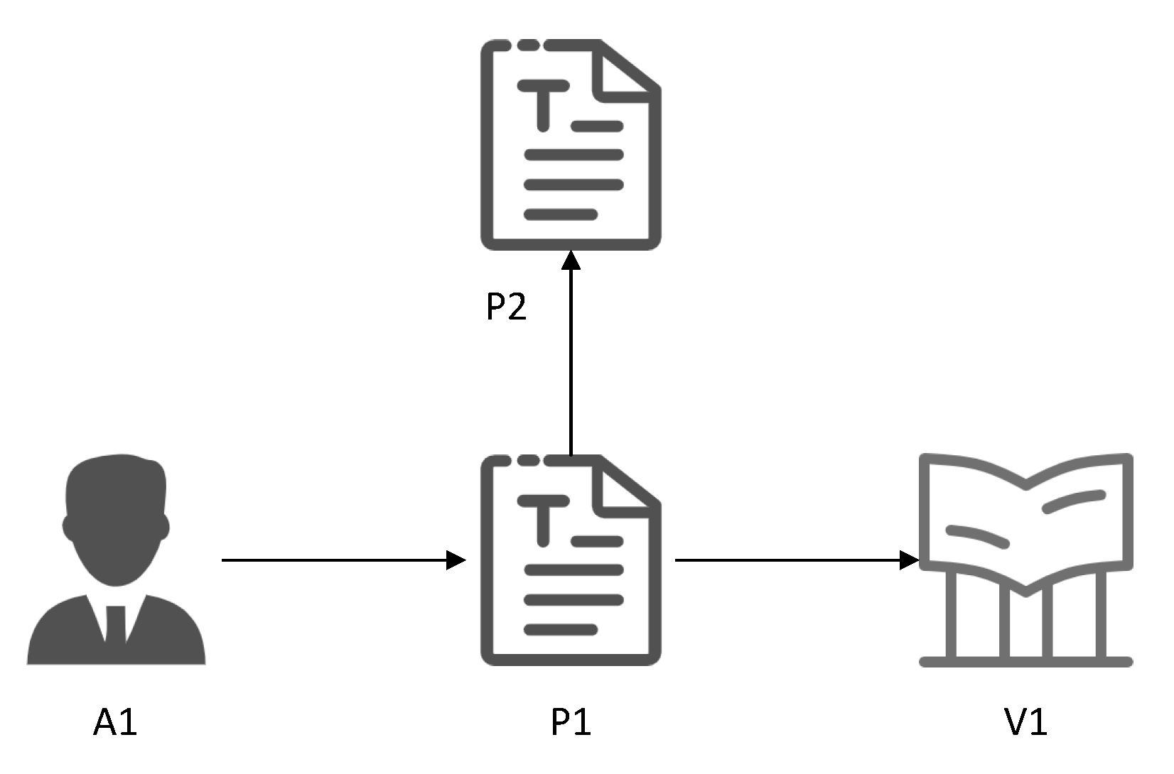
For example, the academic network shown in Figure 1 is a toy example of a heterogeneous graph. There are three types of nodes, including author (A), paper (P), and venue (V). There are also three types of edges, including authors writing papers, papers citing papers, and papers published in a venue.

Figure 1.
The toy example of the academic network. Here the three links represent three edge types.
Problem 1.
Representation learning on heterogeneous graph: Given a heterogeneous network , the goal of heterogeneous graph representation learning is to learn a mapping function , which maps each node to a vector in the d-dimensional space , and .
The symbols used in this paper and the descriptions are shown in Table 2.
Table 2.
The notations in this paper.
4. MSGCN Framework
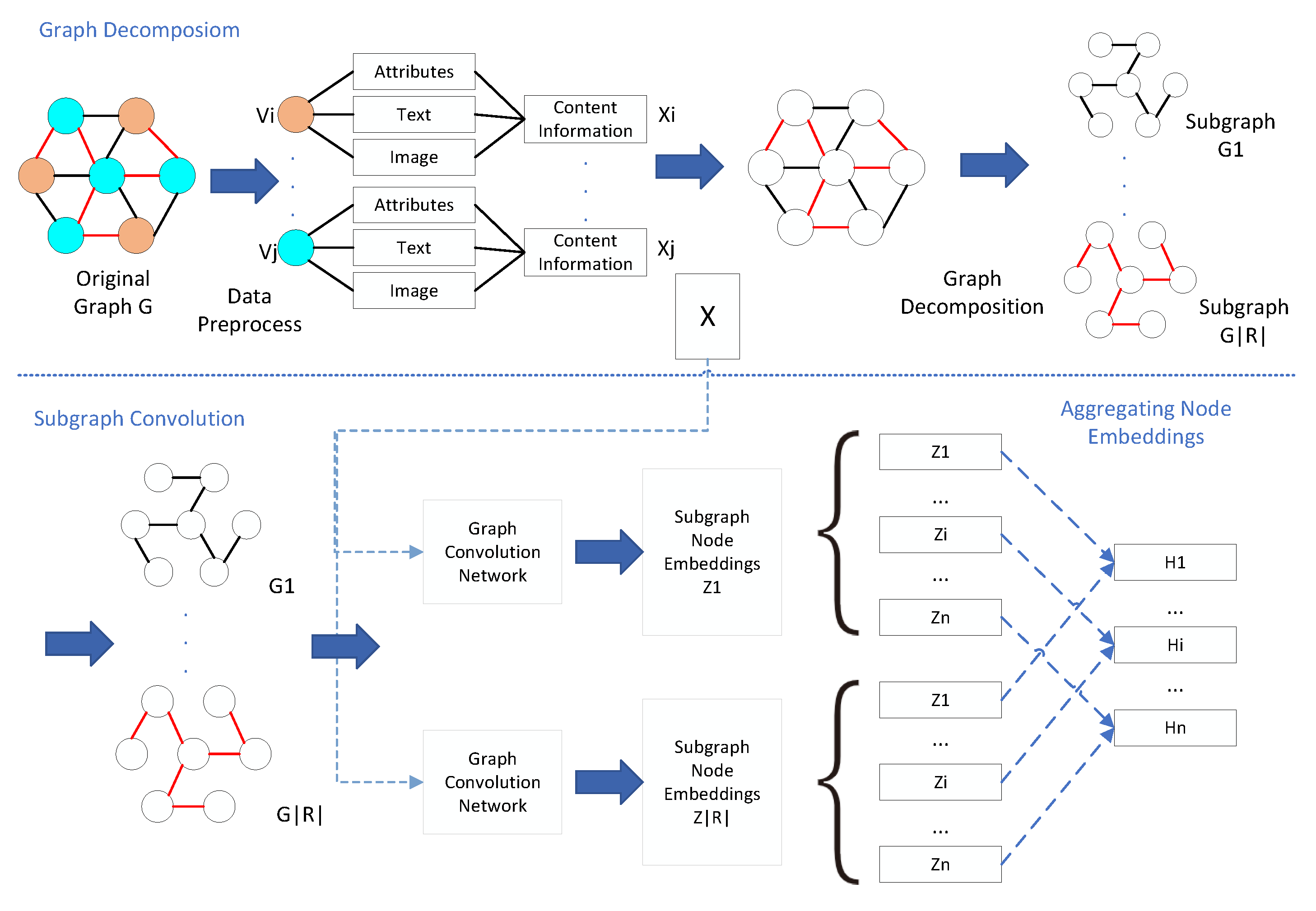
This part mainly introduces the model proposed in this paper, which is composed of original graph decomposition, subgraph convolution, and aggregating node representations. The overall network framework is shown in Figure 2. Apart from the MSGCN framework, we do research on inductive learning tasks to explore how to achieve node embeddings for new nodes efficiently.

Figure 2.
MSGCN model: We first preprocess the node content information, so that they have the same dimension. Then the original graph can be decomposed with respect to the type of edges. For each subgraph, we use graph convolution to get the node representations. Finally, an aggregation operation is applied to get the final representations.
4.1. Original Graph Decomposition
Considering many graph embedding models comprehensively, those models that use node feature information tend to get stronger embedding representations. In order to use the graph neural network to obtain the embeddings, the data must be preprocessed firstly. All methods need to ensure that the data on each node has the same dimension. Real data often have different content information. For example, some nodes may have text information, image information, or attribute information, while others may have multiple types of information. Using this content information directly is inconvenient because the dimensions of each type of content information are different. Therefore, it is necessary to unify all types of information into the same space.
For different types of information, different methods are used to map them to a common space with the same dimension. For example, a convolutional neural network is used for image information and word2vec [42] is used for text information. Then we can use average pooling to get the feature information X that will be input into the model. However, if the nodes have the same dimension of content information, or even if they have only one type of content information, then this step will be much easier.
where represents the content information of i-th type information. X represents the aggregated node content information matrix, which will be used as the input of MSGCN model.
For partial datasets with no content information, we choose to randomly initialize a content matrix X. Note the content matrix X is shared in the following steps.
Given a original heterogeneous graph , and there are n edge types R, i.e., . Supposing the type of each edge is already known, the original heterogeneous graph G is decomposed into n subgraphs:
where each subgraphs can be viewed as a homogeneous graph. In this way, we can successfully solve the heterogeneity of nodes and edges.
For each in , .
4.2. Subgraph Convolution
This part is to get the representation vector of each node in each subgraph. Since the operation of each subgraph is the same, we can take the subgraph as an example. We use a multi-layer graph convolution network for the subgraph , as shown in the following equation
where l is the layer of the graph convolutional network, and the total number L is usually 2. X, the content information matrix, is shared among all the subgraphs. The input of the model is . The output of the model is . is the adjacency matrix of the subgraph . is the activation function. We usually select in the middle layer. The activation function for the last layer is a softmax function. and are weight matrices that are used at each level and they are learnable parameters. Finally, the two-layer graph neural network for is as follows:
is the node representation obtained by the subgraph through the two-layer graph convolution network, aggregating the information of neighbors which are associated with the i-th edge type.
4.3. Aggregating Node Representations
In the subgraph convolution step, each subgraph outputs the representation matrix .
After obtaining the representation matrix of each subgraph, we take the aggregation operation to get the final node embedding representation , as shown in Equation (5):
where weight is determined according to the number of edges of each subgraph. The equation of calculating is given as follows:
The experimental results show that the weight allocation method is unreasonable. For each node , the influence of each subgraph, that is, each edge type, on the node is different. Therefore, we cannot simply calculate the weight of the whole subgraph. For example, comparing one paper quotes another paper with one paper written by an author, we think that the former is more likely to provide the information we want. So for a particular node, some edge types are important, while some edge types have a much lower impact on that node. Accordingly, the weight of each subgraph should be different when the center node aggregates information from subgraphs.
When determining the weight of each subgraph (edge type) on each node, we choose the method based on the number of edges. For each node , the final node representation is defined in Equation (7):
where represents the degree matrix of the subgraph , is the node representation matrix of . Here i indicates which subgraph it belongs to, and j indicates which node it is. So we can get the final representation of H for all the nodes. The node representations obtained by this method can not only retain the topology information of the network, but also the semantic information of the network and the content information of the nodes, which is very comprehensive.
4.4. Model Optimization
We adopt the cross entropy to evaluate model performance. The loss function is defined as follows:
where for each node, for the number of labels for a multi-label classification task. H is the node representation of the output, and y is the label. Then the algorithm of the MSGCN model is shown in Algorithm 1.
| Algorithm 1: MSGCN Model. |
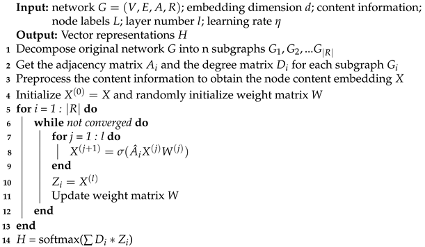 |
5. Application of the Model
In achieving the goal of getting a node representation, we typically encounter two situations. The first is to get the representations of nodes when given nodes and other auxiliary information. The second is we have got some representations of nodes. When new nodes appear, we want to get their representations. These two situations are also known as transductive learning and inductive learning.
5.1. Transductive Learning Task
In this situation, nodes and other information are given, then we can obtain node representations. This is the problem addressed in Section 4 of the article. Given the nodes and edges, we also have the node feature information, node label information, and node and edge type information. Then with the help of the MSGCN model, we get the node representations of all nodes. This is what almost all models work on, but it does not solve all problems.
5.2. Inductive Learning Task
In reality, new nodes are often input into the original network, which can be regarded as a dynamic network. Most dynamic network embedding methods obtain the representation of each node by modeling the dynamics of the network structure. However, the dynamics of network structure depend only on the appearance or disappearance of edges, regardless of the change of nodes. In order to get a representation of the new node, one way is to input the entire dataset containing the old and new nodes into the model for training, but the parts that have already been trained have to be retrained. To solve this problem, it is important to get the representations of the new input node from the existing nodes, which is part of this article.
The MSGCN model has obtained the vector representation of all known nodes, on which the inductive learning task can be carried out. That is, the vector representations of the existing node are used to obtain the new node representations. The reason we can use the representations of known nodes to get the representations of new nodes is that a node tends to have a close relationship with its neighbors. In the case of citation networks, there is a high chance that scholars in one field of research will produce papers that remain in the same field. A large proportion of the papers cited in a paper are still in the same field. So, we can determine the label of the node according to its neighbors, and here we only consider the one-hop neighbors.
For each new node , a neighbor set of fixed size m is sampled to obtain a matrix . The representation of each new node is shown in Equation (9), and the representation of the new node is obtained through the aggregation of neighbor nodes’ information.
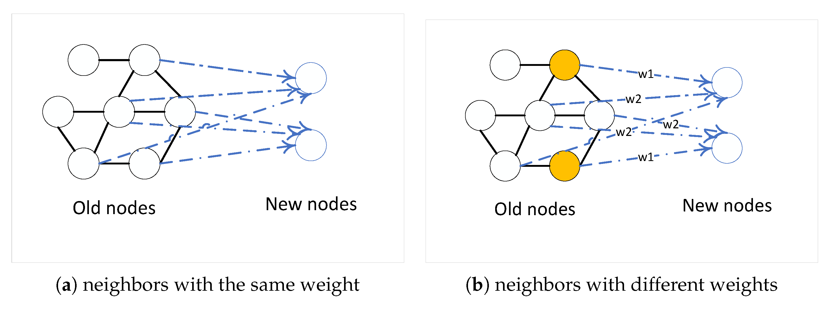
As shown in Figure 3, the new node representation can be obtained directly without the need to retrain the old node, which saves a lot of time. The sampling method here refers to the GraphSAGE model. For nodes with more than m neighbors, random sampling is performed. For nodes with fewer than m neighbors, repeat the sampling until m neighbors are collected. This allows each node to have the same number of neighbors and makes it easier to aggregate.
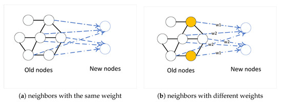
Figure 3.
Inductive learning task. Here the node embeddings of new nodes are achieved by aggregating existing nodes’ embeddings. (a) assumes that all neighbors are of the same role, while (b) first distinguishes which nodes are important, thereby assigning greater weights during aggregation.
However, this method also has some shortcomings. At the beginning of the induction learning task, the neighbors of the nodes sampled are all obtained through the MSGCN model, and the representation of new nodes also has a good effect. However, in this task, we do not use the feature information of nodes, but only obtain the representation vector by aggregating the information of neighbors. Without the help of feature information, the effect in the downstream task will also be deficient. Additionally, the experiment also proved that the accuracy of label classification in the inductive learning task is actually slightly lower than that directly trained by the MSGCN model.
To improve the accuracy of the inductive learning task, we decide to start with the sampling neighbors. We consider that we can assign different weights to different neighbors. If we can get a set of important nodes, we can improve the accuracy of node classification with the help of this set. Of course, we cannot just use this node set. Because other neighbors can also affect the result, even if all neighbors of a node are not in the set. How to distinguish which nodes are important. Intuitively, important nodes should have large degrees. However, assigning large weights directly to these nodes does not seem to be persuasive. However, if a node is important to many other nodes, then we can consider it an important node. With the help of the attention mechanism, we can obtain the attention matrix , which reflects the importance between each node pair. For a center node and a neighbor , self-attention is performed to compute attention coefficient . Then we use the softmax function to normalize all the neighbors:
where h is the node feature, is the neighborhood of node in the graph, W and a are trainable parameters. Then a matrix, , of attention coefficient is achieved. Here we choose as the activation function. is very similar to , they can solve the gradient vanishing problem. When the input x is less than 0, will be 0, while will be a negative value. The benefit of using is that the gradient can also be calculated for the part of the input that is less than 0 during the backpropagation process, avoiding the gradient direction sawtooth problem. So we choose as the activation function.
For each node, we choose its top k important neighbors, thus we can get a new matrix , which records the index of the k most important neighbors of each node. The value of k is not suitable to be large, because many nodes have few neighbors and too many unimportant nodes will be taken into account, which is similar to using the degree matrix directly. At the same time, it should not be too small, so that it can include as many important nodes as possible.
A node is important if it appears many times in the matrix as an important neighbor. We count the occurrence times of each node, and the node exceeding a threshold value is regarded as an important node. We set the weight to for important nodes and for unimportant nodes. For a new node , as we say before, we sample m neighbors. Here we have important neighbors and unimportant neighbors, and . The representation can be achieved in Equation (13): -4.6cm0cm
Since the representations of new nodes are obtained based on existing nodes, it is reasonable that the accuracy will not outperform the MSGCN framework. However, it is worth sacrificing a little accuracy for time.
Although the accuracy is slightly lower than the direct training of the MSGCN model, in fact, the accuracy is still higher than most models. However, as time goes by, the latest nodes in the future will be neighbors of those nodes with lower accuracy, so the accuracy will further decline. However, the number of new nodes in our experiment is the same as the number of trained nodes in MSGCN, so the effect of the inductive task can still be guaranteed in the short term. However, in order to maintain accuracy, when there are enough new nodes, it is better to use the MSGCN model to train all the data.
6. Experiment
6.1. Dataset
The datasets used in this paper are the same three datasets as the MuSDAC [43] model. They are ACM [44], AMiner, and DBLP [12]. ACM is a huge bibliographic database containing books, journals, and papers from key publishing houses in the computer field. AMiner is a new-generation technology intelligence analysis and mining platform established by the Department of Computer Science and Technology of Tsinghua University. DBLP is an integrated computer database system of English literature with authors as the core of research achievements in the computer field. The data of these datasets are shown in Table 3. The data of the three datasets are the same in the number of nodes, but the number of edges is very different. Therefore, the results obtained by different methods on these three datasets are quite different.
Table 3.
Datasets.
6.2. Baselines
The following is a list of comparative experiments with this paper to verify the validity of our proposed model. For those methods based on homogeneous graphs, we processed the data and ignored the heterogeneity of nodes and edges. We use OpenNMS framework and DGL framework, which contain many graph embedding methods, to run most of the contrast models. In addition, a variant MSGCN-mean of this model is also compared. The brief introduction of these contrast models are as follows:
- DeepWalk [3]: A random-walk-based embedding method designed for the same composition, which performs truncated random-walk over the network and is represented by skip-Gram model learning nodes.
- Graph Factorization (GF) [37]: A method of obtaining embedding by decomposing the adjacency matrix of a graph.
- SDNE [23]: Uses an automatic encoder to embed graph nodes and capture highly nonlinear dependencies.
- HOPE [22]: A method that uses generalized singular value decomposition (SVD) to get embeddings efficiently.
- GCN [7]: A classic semi-supervised graph neural network designed for the same composition, aggregating neighborhood information.
- GAT [8]: A neural network approach that applies the mechanism of attention to the same composition.
- TAGCN [45]: TAGCN is one of the variants of GCN. It uses a K graph convolution kernel to extract local features of different sizes.
- HAN [12]: A semi-supervised graph neural network embedding method for heterogeneous graphs that uses node-level attention and semantic attention to aggregate neighborhood information.
- MuSDAC [43]: A method on heterogeneous information networks.
- GraphInception [46]: A deep GCN for collective classification on heterogeneous information networks.
- MSGCN-mean: A variant of MSGCN that simply averages the representation of each node without considering the effect of edges on each node.
In this paper, as we conduct experiments on the multi-class classification task, we choose accuracy as the evaluation metric to measure the performance of each model.
6.3. The Experimental Setup
For this MSGCN method, we randomly initialize the weight matrices. We set the learning rate to be 0.005, dropout to be 0.5, and weight attenuation to be 0.0005. Considering the three datasets, we set the number of epochs to 1000. Just like the paper of GCN, we perform a semi-supervised learning task and only 10% of the nodes are labeled during the training. In the subsequent inductive learning task, 10 first-order neighbors are selected for each new node.
6.4. Multi-Class Node Classification
We carried out experiments on multi-class node classification tasks. Contrast experiments include classic graph embedding methods, homogeneous GNN methods, and some heterogeneous graph methods. As we can see in Table 4, the proposed MSGCN and its variant MSGCN-mean outperform the other baselines on three datasets. In ACM and AMiner datasets, the density of edges is relatively sparse and the number of edges is small, so the weight does not bring much help. However, in the DBLP dataset, because of the high density, each node is related to multiple edges in each subgraph, and the weight also has a significant impact on the experimental results. We can conclude that MSGCN is more suitable for dense graphs than MSGCN-mean.
Table 4.
Experimental results.
Most of the contrast models like DeepWalk and Graph Factorization use neither feature information nor use semantic information. As a result, these models do not perform very well. In contrast, GCN and GAT take feature information into consideration, and HAN is the only one that uses semantic information. However, our MSGCN model takes full advantage of all the information, which is the reason why the accuracy is higher than theirs.
Instead of using metapaths, MSGCN decomposes the original graph based on edge types. Doing so can actually take some advantage of the metapath-based methods. For example, the author writes a paper can be an edge type. Based on this edge type, we can get a decomposed subgraph, where each edge can represent an author writes a paper. Therefore, there are many metapaths in this subgraph, like an author writes a paper(), two authors write a paper together (), and two papers are all written by the same author (). Other information like the relation between papers and venues can be obtained in other subgraphs. We can find that the MSGCN model has the advantages of the metapath-based methods while also making full use of all aspects of information.
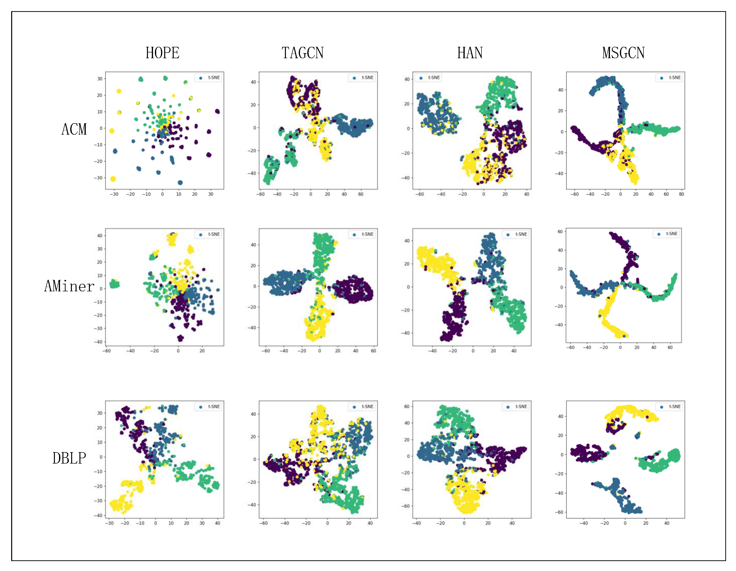
In order to better reflect the superiority of our model in the node classification task, for each category we select one with the best experimental result along with our MSGCN model, to show the visualization results. Here we choose HOPE for the classic graph embedding methods, TAGCN for homogeneous GNN methods, and HAN for heterogeneous graph methods. The experimental results are shown in Figure 4. We can find that these models can achieve good results in node classification. However, many nodes in comparison models are ambiguous, so it is not clear which cluster these nodes should belong to. In contrast, although the MSGCN model cannot classify all the nodes correctly, it can get a more obvious result with higher accuracy.
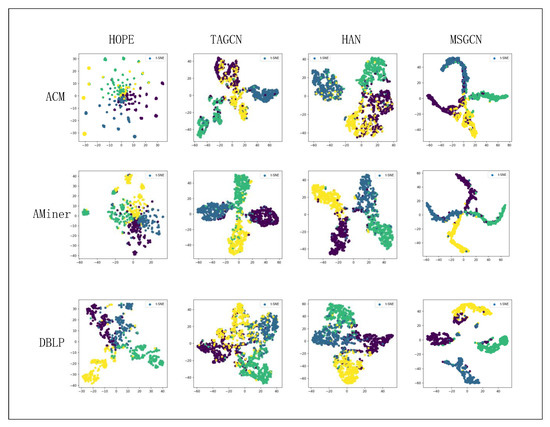
Figure 4.
The visualization results of the models. Models include HOPE, TAGCN, HAN, and MSGCN. We conduct experiment on node classification task on three dataset. The visualization results demonstrate the superiority of our model.
6.5. Inductive Learning Task
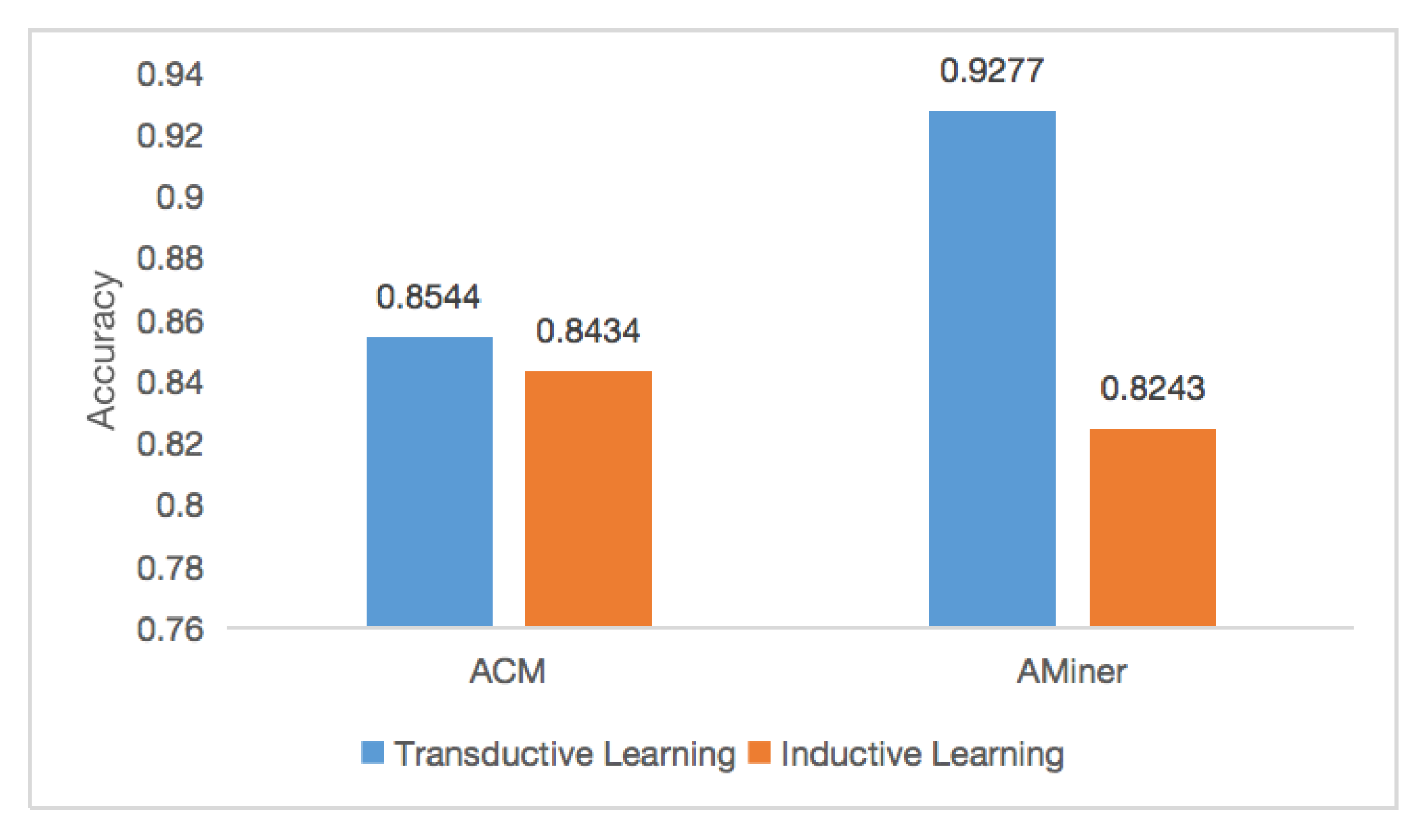
After analyzing three datasets, we find the DBLP is too dense, in which the neighbors of each node have more than 500 neighbors on average. So we verify the performance of models on ACM and AMiner datasets. The experimental results are shown in Figure 5. It can be seen that the accuracy is still over 80%, slightly lower than the result obtained by direct training with the MSGCN model.
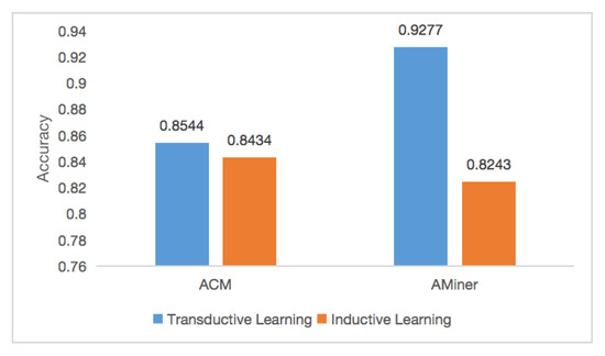
Figure 5.
The experimental result of the inductive learning task. The accuracy is little lower than that of the MSGCN model.
At the beginning of the induction learning task, the neighbors of the nodes sampled are all obtained through the MSGCN model, and the representation of new nodes also has a good effect. However, in this task, we do not use the feature information of nodes, but only obtain the representation vector by aggregating the information of neighbors. Without the help of feature information, the effect in the downstream task will also be deficient. Additionally, the experiment also proves that the accuracy of label classification in the inductive learning task is actually slightly lower than that directly trained by the MSGCN model.
In spite of this, in fact, the accuracy is still higher than that of most models. However, as time goes by, the latest nodes in the future will be neighbors of those nodes with lower accuracy, so the accuracy will further decline. However, the number of new nodes in our experiment is the same as the number of trained nodes in MSGCN, so the effect of the inductive task can still be guaranteed in the short term. However, in order to maintain accuracy, when enough new nodes appear, it is better to use the MSGCN model to train all the data. Because the feature information is used in MSGCN, retraining ensures that the inductive task remains accurate for a long time.
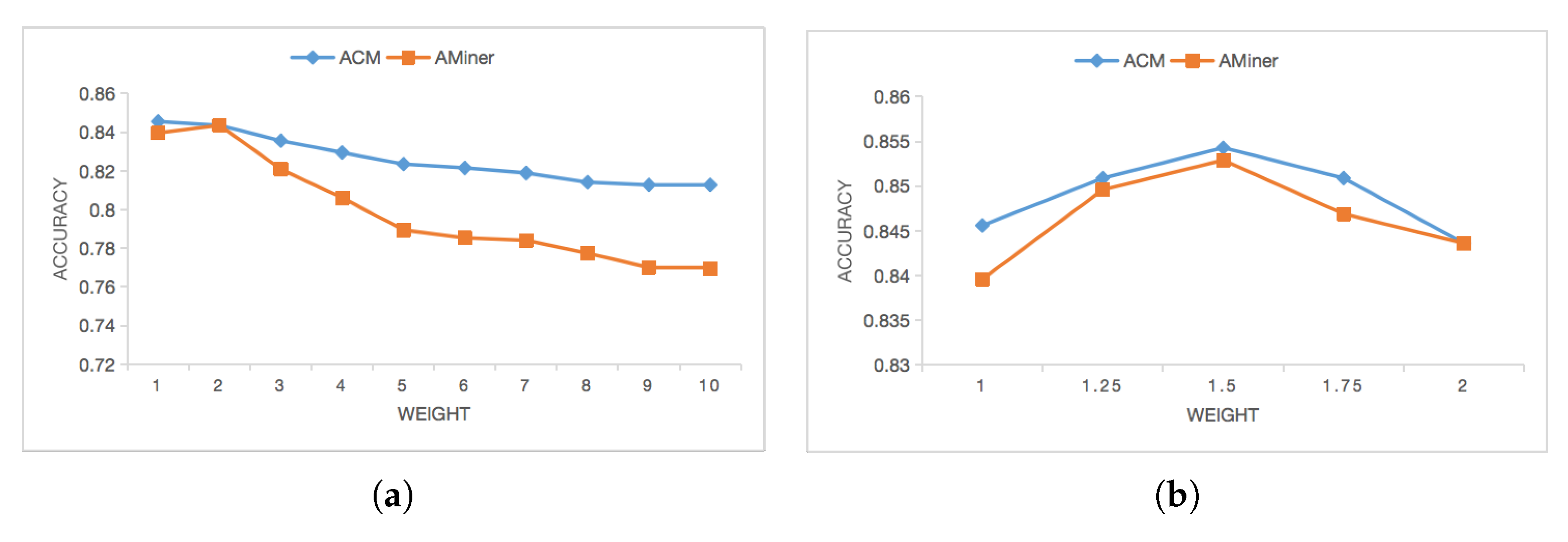
After that, we fine-tune the experimental settings only to explore the influence of assigning different weights to important nodes on the accuracy in the node classification task of new nodes. We consider the nodes that occur more than 10 times in the sampling matrix M as important nodes. The default initial weight of all nodes is 1. The experimental results are shown in Figure 6. It can be seen that assigning an appropriately high weight to important nodes will indeed improve the accuracy of node classification, but the weight should not be too high. Numerous experiments have shown that 1.5 is an appropriate weight.
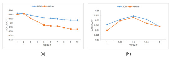
Figure 6.
(a) Weight range from 1 to 10. (b) Weight range from 1 to 2. The experimental result of the inductive learning task. It reflects the influence of assigning different weights to important nodes on the accuracy in the node classification task of new nodes.
6.6. Extended Experiment
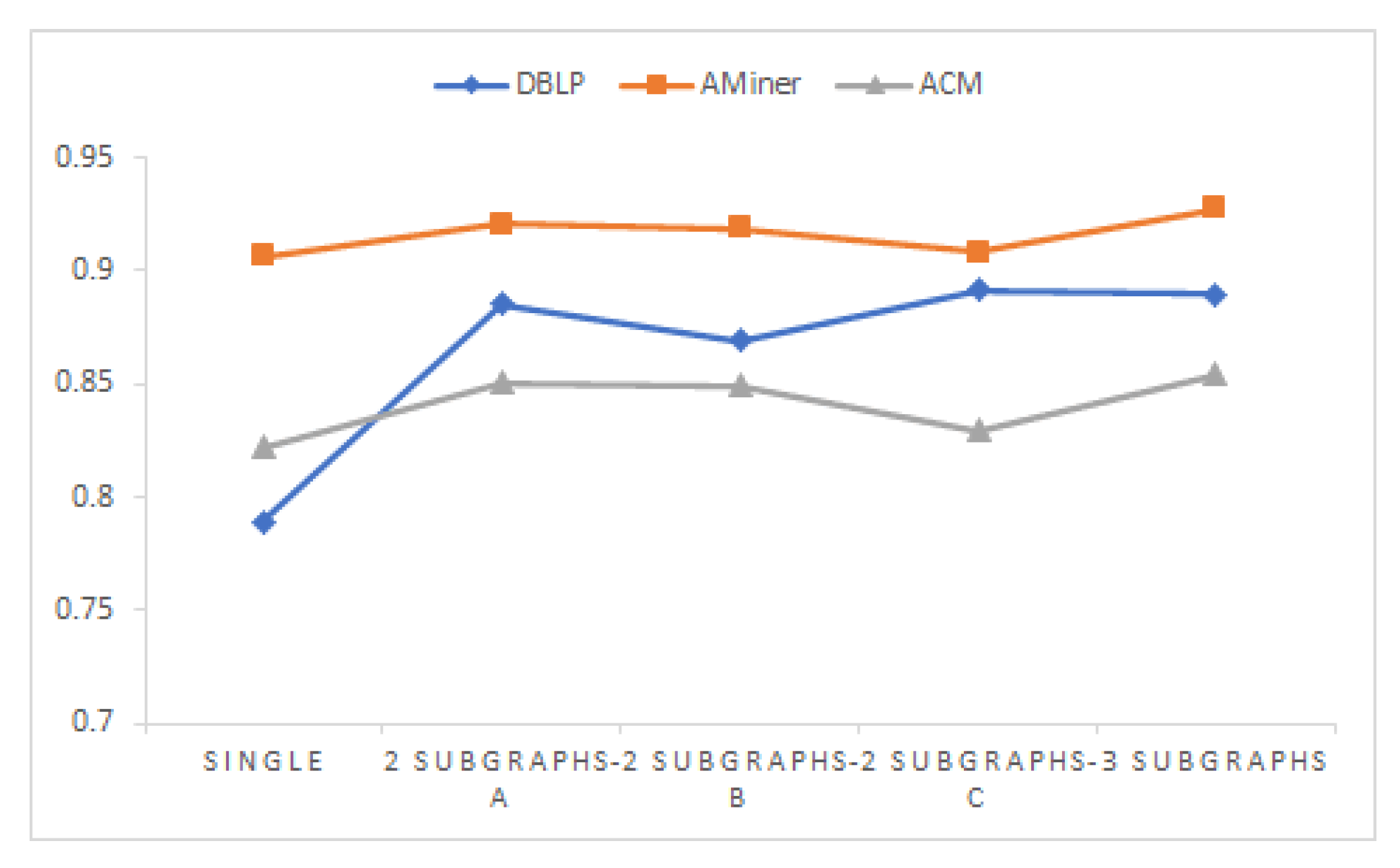
In order to examine the influence of the number of subgraphs on the experiment, we conducted an extended experiment. For the previous three datasets, since they all have three types of edges, they are all divided into three subgraphs. In order to explore the influence of the number of subgraphs on the results, we combine the two types of edges.
We used the given three datasets to perform experiments on a single graph and two subgraphs to compare the results of experiments divided into three subgraphs. In the case of a single graph, the heterogeneity of nodes and edges is ignored and regarded as a compositional graph, which can be understood as a convolutional neural network. In the case of two graphs, we treat the two types of edges the same. So for every dataset, there are three possible scenarios. We fully considered the three cases and conducted experiments under the same parameters. There are five cases in total, and the experimental result is shown in Figure 7.
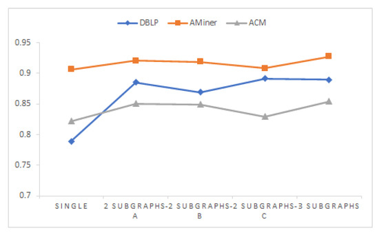
Figure 7.
The result of the extended experiment. The number of subgraphs have influence on the result.
It can be seen from the figure that, for the three datasets, the three-sub-graph has the best experimental effect, while the single-graph has the worst effect. Therefore, we can conclude that our method can be used on heterogeneous graphs with multiple types of nodes and edges.
7. Conclusions
In this paper, a new graph representation learning model MSGCN is proposed for heterogeneous graphs. We decompose the original graph into multiple subgraphs so that we can take the semantic information into consideration, which takes advantage of the metapath-based methods and obtains better results. When considering the application of the model, we also design the inductive learning module to cope with the unseen nodes. A new node sampling method, which assigns weights to neighbors, is also designed to improve the experimental effect. To verify the validity of the model, we conduct experiments on ACM, AMiner, and DBLP datasets. The experimental results show that the model is feasible and superior. In this paper, we ignore the time information of the node. Actually, time information plays a key role in the network. For example, the research interest of a researcher will change over time. Accordingly, we will extend our method to deal with this issue in future work.
Author Contributions
Conceptualization, J.C.; methodology, J.C.; software, J.C.; validation, J.C., F.H. and J.P.; formal analysis, J.C.; investigation, J.C.; resources, J.C.; data curation, J.C.; writing—original draft preparation, J.C.; writing—review and editing, J.C., F.H. and J.P.; visualization, J.C.; supervision, J.C.; project administration, J.P.; funding acquisition, J.P. All authors have read and agreed to the published version of the manuscript.
Funding
This work was supported in part by the Sichuan Science and Technology Program under Grant 2018GZDZX0010, Grant 2019YFG0494 and Grant 2020YFG0308.
Institutional Review Board Statement
Not applicable.
Informed Consent Statement
Not applicable.
Conflicts of Interest
The authors declare no conflict of interest.
References
- Hamilton, W.L.; Ying, R.; Leskovec, J. Representation learning on graphs: Methods and applications. arXiv 2017, arXiv:1709.05584. [Google Scholar]
- Yi, P.; Huang, F.; Peng, J. A Fine-grained Graph-based Spatiotemporal Network for Bike Flow Prediction in Bike-sharing Systems. In Proceedings of the 2021 SIAM International Conference on Data Mining (SDM), Virtual, 29 April–1 May 2021; pp. 513–521. [Google Scholar]
- Perozzi, B.; Al-Rfou, R.; Skiena, S. Deepwalk: Online learning of social representations. In Proceedings of the 20th ACM SIGKDD International Conference on Knowledge Discovery and Data Mining, KDD ’14, New York, NY, USA, 24–27 August 2014; pp. 701–710. [Google Scholar]
- Grover, A.; Leskovec, J. node2vec: Scalable feature learning for networks. In Proceedings of the ACM SIGKDD International Conference on Knowledge Discovery and Data Mining, San Francisco, CA, USA, 13–17 August 2016; pp. 855–864. [Google Scholar]
- Tang, J.; Qu, M.; Wang, M.; Zhang, M.; Yan, J.; Mei, Q. LINE: Large-scale information network embedding. In Proceedings of the 24th International Conference on World Wide Web, WWW 2015, Florence, Italy, 18–22 May 2015; pp. 1067–1077. [Google Scholar]
- Hamilton, W.L.; Ying, Z.; Leskovec, J. Inductive representation learning on large graphs. In Proceedings of the Advances in Neural Information Processing Systems 30: Annual Conference on Neural Information Processing Systems 2017, Long Beach, CA, USA, 4–9 December 2017; pp. 1024–1034. [Google Scholar]
- Kipf, T.N.; Welling, M. Semi-supervised classification with graph convolutional networks. In Proceedings of the 5th International Conference on Learning Representations, ICLR 2017, Toulon, France, 24–26 April 2017. [Google Scholar]
- Velickovic, P.; Cucurull, G.; Casanova, A.; Romero, A.; Liò, P.; Bengio, Y. Graph attention networks. In Proceedings of the 6th International Conference on Learning Representations, ICLR 2018, Vancouver, BC, Canada, 30 April–3 May 2018. [Google Scholar]
- Dong, Y.; Hu, Z.; Wang, K.; Sun, Y.; Tang, J. Heterogeneous network representation learning. In Proceedings of the Twenty-Ninth International Joint Conference on Artificial Intelligence, IJCAI 2020, Yokohama, Japan, 11–17 July 2020; pp. 4861–4867. [Google Scholar]
- Shi, C.; Li, Y.; Zhang, J.; Sun, Y.; Yu, P.S. A survey of heterogeneous information network analysis. IEEE Trans. Knowl. Data Eng. 2017, 29, 17–37. [Google Scholar] [CrossRef]
- Cen, Y.; Zou, X.; Zhang, J.; Yang, H.; Zhou, J.; Tang, J. Representation learning for attributed multiplex heterogeneous network. In Proceedings of the 25th ACM SIGKDD International Conference on Knowledge Discovery & Data Mining, KDD 2019, Anchorage, AK, USA, 4–8 August 2019; pp. 1358–1368. [Google Scholar]
- Wang, X.; Ji, H.; Shi, C.; Wang, B.; Ye, Y.; Cui, P.; Yu, P.S. Heterogeneous graph attention network. In Proceedings of the World Wide Web Conference, WWW 2019, San Francisco, CA, USA, 13–17 May 2019; pp. 2022–2032. [Google Scholar]
- Shi, C.; Hu, B.; Zhao, W.X.; Yu, P.S. Heterogeneous information network embedding for recommendation. IEEE Trans. Knowl. Data Eng. 2019, 31, 357–370. [Google Scholar] [CrossRef] [Green Version]
- Zhang, C.; Song, D.; Huang, C.; Swami, A.; Chawla, N.V. Heterogeneous graph neural network. In Proceedings of the 25th ACM SIGKDD International Conference on Knowledge Discovery & Data Mining, KDD 2019, Anchorage, AK, USA,, 4–8 August 2019; pp. 793–803. [Google Scholar]
- Hu, Z.; Dong, Y.; Wang, K.; Sun, Y. Heterogeneous graph transformer. In Proceedings of the WWW ’20: The Web Conference 2020, Taipei, Taiwan, 20–24 April 2020; pp. 2704–2710. [Google Scholar]
- Fu, T.-Y.; Lee, W.-C.; Lei, Z. Hin2vec: Explore meta-paths in heterogeneous information networks for representation learning. In Proceedings of the 2017 ACM on Conference on Information and Knowledge Management, CIKM 2017, Singapore, 6–10 November 2017; pp. 1797–1806. [Google Scholar]
- Zhao, J.; Wang, X.; Shi, C.; Hu, B.; Song, G.; Ye, Y. Heterogeneous graph structure learning for graph neural networks. In Proceedings of the Thirty-Fifth AAAI Conference on Artificial Intelligence, AAAI 2021, Thirty-Third Conference on Innovative Applications of Artificial Intelligence, IAAI 2021, The Eleventh Symposium on Educational Advances in Artificial Intelligence, EAAI 2021, Virtual Event, 2–9 February 2021; pp. 4697–4705. [Google Scholar]
- Wang, X.; Liu, N.; Han, H.; Shi, C. Self-supervised heterogeneous graph neural network with co-contrastive learning. In Proceedings of the KDD ’21: The 27th ACM SIGKDD Conference on Knowledge Discovery and Data Mining, Virtual Event, Singapore, 14–18 August 2021; pp. 1726–1736. [Google Scholar]
- Adhikari, B.; Zhang, Y.; Ramakrishnan, N.; Prakash, B.A. Distributed representations of subgraphs. In Proceedings of the 2017 IEEE International Conference on Data Mining Workshops (ICDMW), New Orleans, LA, USA, 18–21 November 2017; pp. 111–117. [Google Scholar]
- Yuan, C.; Li, J.; Zhou, W.; Lu, Y.; Zhang, X.; Hu, S. Dyhgcn: A dynamic heterogeneous graph convolutional network to learn users’ dynamic preferences for information diffusion prediction. In Proceedings of the Machine Learning and Knowledge Discovery in Databases - European Conference, ECML PKDD 2020, Ghent, Belgium, 14–18 September 2020; pp. 347–363. [Google Scholar]
- Cao, S.; Lu, W.; Xu, Q. Grarep: Learning graph representations with global structural information. In Proceedings of the Proceedings of the 24th ACM International Conference on Information and Knowledge Management, CIKM 2015, Melbourne, VIC, Australia, 19–23 October 2015; pp. 891–900. [Google Scholar]
- Ou, M.; Cui, P.; Pei, J.; Zhang, Z.; Zhu, W. Asymmetric transitivity preserving graph embedding. In Proceedings of the 22nd ACM SIGKDD International Conference on Knowledge Discovery and Data Mining, San Francisco, CA, USA, 13–17 August 2016; pp. 1105–1114. [Google Scholar]
- Wang, D.; Cui, P.; Zhu, W. Structural deep network embedding. In Proceedings of the 22nd ACM SIGKDD International Conference on Knowledge Discovery and Data Mining, San Francisco, CA, USA, 13–17 August 2016; pp. 1225–1234. [Google Scholar]
- Dong, Y.; Chawla, N.V.; Swami, A. metapath2vec: Scalable representation learning for heterogeneous networks. In Proceedings of the 23rd ACM SIGKDD International Conference on Knowledge Discovery and Data Mining, Halifax, NS, Canada, 13–17 August 2017; pp. 135–144. [Google Scholar]
- Adhikari, B.; Zhang, Y.; Ramakrishnan, N.; Prakash, B.A. Sub2vec: Feature learning for subgraphs. In Pacific-Asia Conference on Knowledge Discovery and Data Mining; Springer: Berlin/Heidelberg, Germany, 2018. [Google Scholar]
- Narayanan, A.; Chandramohan, M.; Chen, L.; Liu, Y.; Saminathan, S. subgraph2vec: Learning distributed representations of rooted sub-graphs from large graphs. arXiv 2016, arXiv:1606.08928. [Google Scholar]
- Tang, J.; Qu, M.; Mei, Q. PTE: Predictive text embedding through large-scale heterogeneous text networks. In Proceedings of the 1th ACM SIGKDD International Conference on Knowledge Discovery and Data Mining, Sydney, NSW, Australia, 10–13 August 2015; pp. 1165–1174. [Google Scholar]
- Wang, M.; Lin, Y.; Lin, G.; Yang, K.; Wu, X. M2GRL: A multi-task multi-view graph representation learning framework for web-scale recommender systems. In Proceedings of the KDD ’20: The 26th ACM SIGKDD Conference on Knowledge Discovery and Data Mining, Virtual Event, CA, USA, 23–27 August 2020; pp. 2349–2358. [Google Scholar]
- Mahdavi, S.; Khoshraftar, S.; An, A. dynnode2vec: Scalable dynamic network embedding. In Proceedings of the International Conference on Big Data, Big Data 2018, Seattle, WA, USA, 10–13 December 2018; pp. 3762–3765. [Google Scholar]
- Pareja, A.; Domeniconi, G.; Chen, J.; Ma, T.; Suzumura, T.; Kanezashi, H.; Kaler, T.; Schardl, T.B.; Leiserson, C.E. Evolvegcn: Evolving graph convolutional networks for dynamic graphs. In Proceedings of the The Thirty-Fourth AAAI Conference on Artificial Intelligence, AAAI 2020, The Thirty-Second Innovative Applications of Artificial Intelligence Conference, IAAI 2020, The Tenth AAAI Symposium on Educational Advances in Artificial Intelligence, EAAI 2020, New York, NY, USA, 7–12 February 2020; pp. 5363–5370. [Google Scholar]
- Nguyen, G.H.; Lee, J.B.; Rossi, R.A.; Ahmed, N.K.; Koh, E.; Kim, S. Continuous-time dynamic network embeddings. In Proceedings of the Companion of the The Web Conference 2018 on The Web Conference 2018, WWW 2018, Lyon, France, 23–27 April 2018; pp. 969–976. [Google Scholar]
- Ye, Y.; Hou, S.; Chen, L.; Lei, J.; Wan, W.; Wang, J.; Xiong, Q.; Shao, F. Out-of-sample node representation learning for heterogeneous graph in real-time android malware detection. In Proceedings of the Twenty-Eighth International Joint Conference on Artificial Intelligence, IJCAI 2019, Macao, China, 10–16 August 2019; pp. 4150–4156. [Google Scholar]
- Sankar, A.; Wu, Y.; Gou, L.; Zhang, W.; Yang, H. Dysat: Deep neural representation learning on dynamic graphs via self-attention networks. In Proceedings of the WSDM ’20: The Thirteenth ACM International Conference on Web Search and Data Mining, Houston, TX, USA, 3–7 February 2020; pp. 519–527. [Google Scholar]
- Sen, P.; Namata, G.; Bilgic, M.; Getoor, L.; Gallagher, B.; Eliassi-Rad, T. Collective classification in network data. AI Mag. 2008, 29, 93–106. [Google Scholar] [CrossRef] [Green Version]
- Wang, X.; Cui, P.; Wang, J.; Pei, J.; Zhu, W.; Yang, S. Community preserving network embedding. In Proceedings of the Thirty-First AAAI Conference on Artificial Intelligence, 4–9 February 2017; pp. 203–209. [Google Scholar]
- Goyal, P.; Ferrara, E. Graph embedding techniques, applications, and performance: A survey. Knowl.-Based Syst. 2018, 151, 78–94. [Google Scholar] [CrossRef] [Green Version]
- Ahmed, A.; Shervashidze, N.; Narayanamurthy, S.M.; Josifovski, V.; Smola, A.J. Distributed large-scale natural graph factorization. In Proceedings of the 22nd International World Wide Web Conference, WWW ’13, Rio de Janeiro, Brazil, 13–17 May 2013; pp. 37–48. [Google Scholar]
- Mikolov, T.; Chen, K.; Corrado, G.; Dean, J. Efficient estimation of word representations in vector space. In Proceedings of the 1st International Conference on Learning Representations, ICLR 2013, Scottsdale, Arizona, USA, 2–4 May 2013. [Google Scholar]
- Fu, X.; Zhang, J.; Meng, Z.; King, I. MAGNN: Metapath aggregated graph neural network for heterogeneous graph embedding. In Proceedings of the WWW ’20: The Web Conference 2020, Taipei, Taiwan, 20–24 April 2020; pp. 2331–2341. [Google Scholar]
- Le, Q.V.; Mikolov, T. Distributed representations of sentences and documents. In Proceedings of the 31th International Conference on Machine Learning, ICML 2014, Beijing, China, 21–26 June 2014; pp. 1188–1196. [Google Scholar]
- Xie, Y.; Li, C.; Yu, B.; Zhang, C.; Tang, Z. A survey on dynamic network embedding. arXiv 2020, arXiv:2006.08093. [Google Scholar]
- Rong, X. word2vec parameter learning explained. arXiv 2014, arXiv:1411.2738. [Google Scholar]
- Yang, S.; Song, G.; Jin, Y.; Du, L. Domain adaptive classification on heterogeneous information networks. In Proceedings of the Twenty-Ninth International Joint Conference on Artificial Intelligence, IJCAI 2020, Yokohama, Japan, 11–17 July 2020; pp. 1410–1416. [Google Scholar]
- Kong, X.; Yu, P.S.; Ding, Y.; Wild, D.J. Meta path-based collective classification in heterogeneous information networks. In Proceedings of the 21st ACM International Conference on Information and Knowledge Management, CIKM’12, Maui, HI, USA, 29 October–2 November 2012; pp. 1567–1571. [Google Scholar]
- Du, J.; Zhang, S.; Wu, G.; Moura, J.M.F.; Kar, S. Topology adaptive graph convolutional networks. arXiv 2017, arXiv:1710.10370. [Google Scholar]
- Xiong, Y.; Zhang, Y.; Kong, X.; Chen, H.; Zhu, Y. Graphinception: Convolutional neural networks for collective classification in heterogeneous information networks. IEEE Trans. Knowl. Data Eng. 2021, 33, 1960–1972. [Google Scholar] [CrossRef]
Publisher’s Note: MDPI stays neutral with regard to jurisdictional claims in published maps and institutional affiliations. |
© 2021 by the authors. Licensee MDPI, Basel, Switzerland. This article is an open access article distributed under the terms and conditions of the Creative Commons Attribution (CC BY) license (https://creativecommons.org/licenses/by/4.0/).