
Application of Mode-Adaptive Bidirectional Pushover Analysis to an Irregular Reinforced Concrete Building Retrofitted via Base Isolation


Abstract
:Featured Application
Abstract
1. Introduction
1.1. Background
1.2. Motivation
1.3. Objectives
- Is MABPA capable of predicting the peak response of irregular base-isolated buildings?
- The prediction of the peak equivalent displacement of the first two modal responses is an essential step in MABPA. For this, the relationship between the maximum momentary input energy and the peak displacement needs to be properly evaluated. How can this relationship be evaluated from the pushover analysis results?
- In the prediction of the maximum momentary input energy of the first two modal responses, the effect of simultaneous bidirectional excitation needs to be considered. Can the upper bound of the peak equivalent displacement of the first two modal responses be predicted using the bidirectional maximum momentary input energy spectrum [52]?
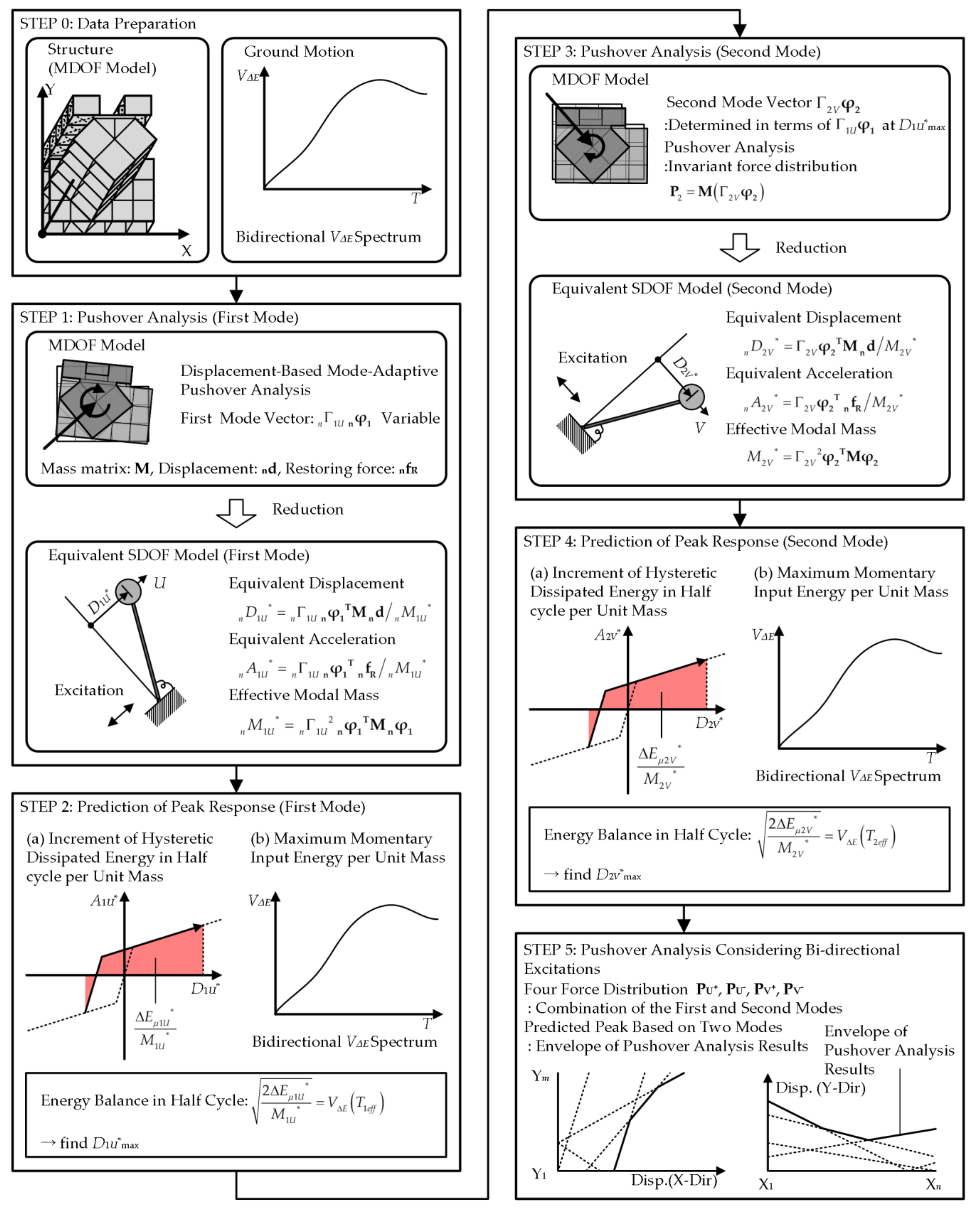
2. Description of MABPA
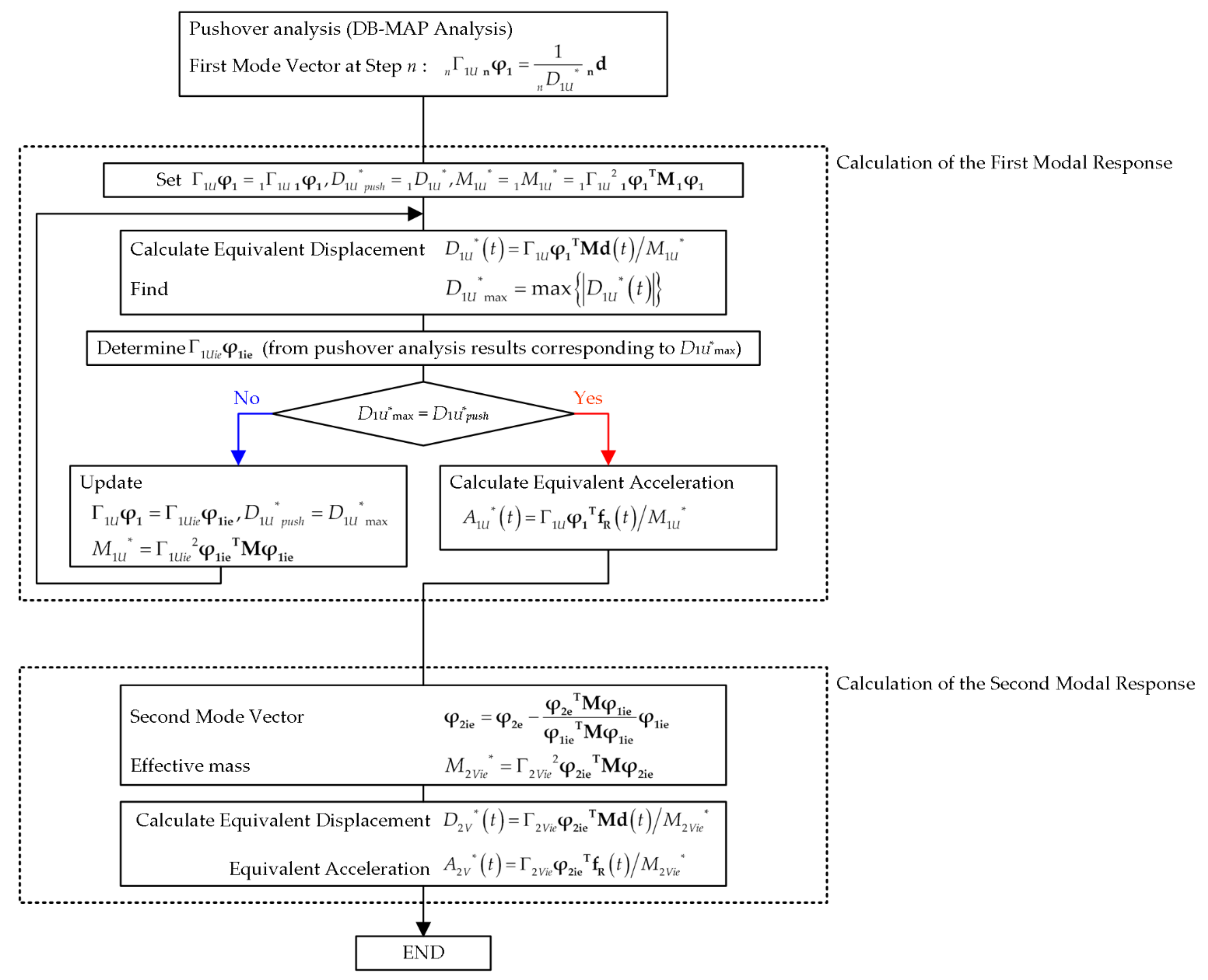
2.1. Outline of MABPA
- The bidirectional momentary input energy proposed in the previous study was applied as the seismic intensity parameter.
- The peak response of each mode was predicted from the energy balance in a half cycle of the structural response.
2.2. Prediction of the Peak Response using the Momentary Energy Input
2.2.1. Calculation of the Bidirectional Momentary Input Energy Spectrum
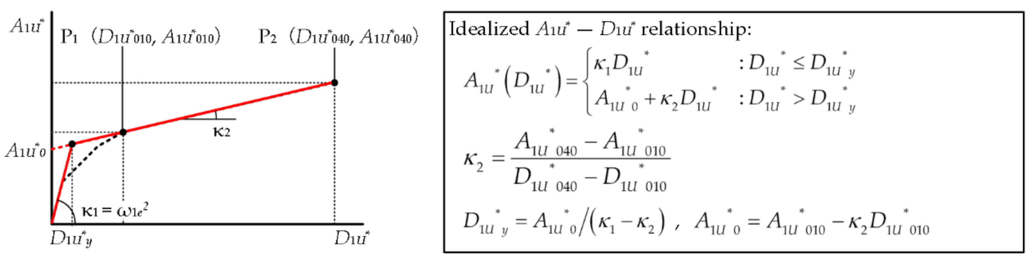
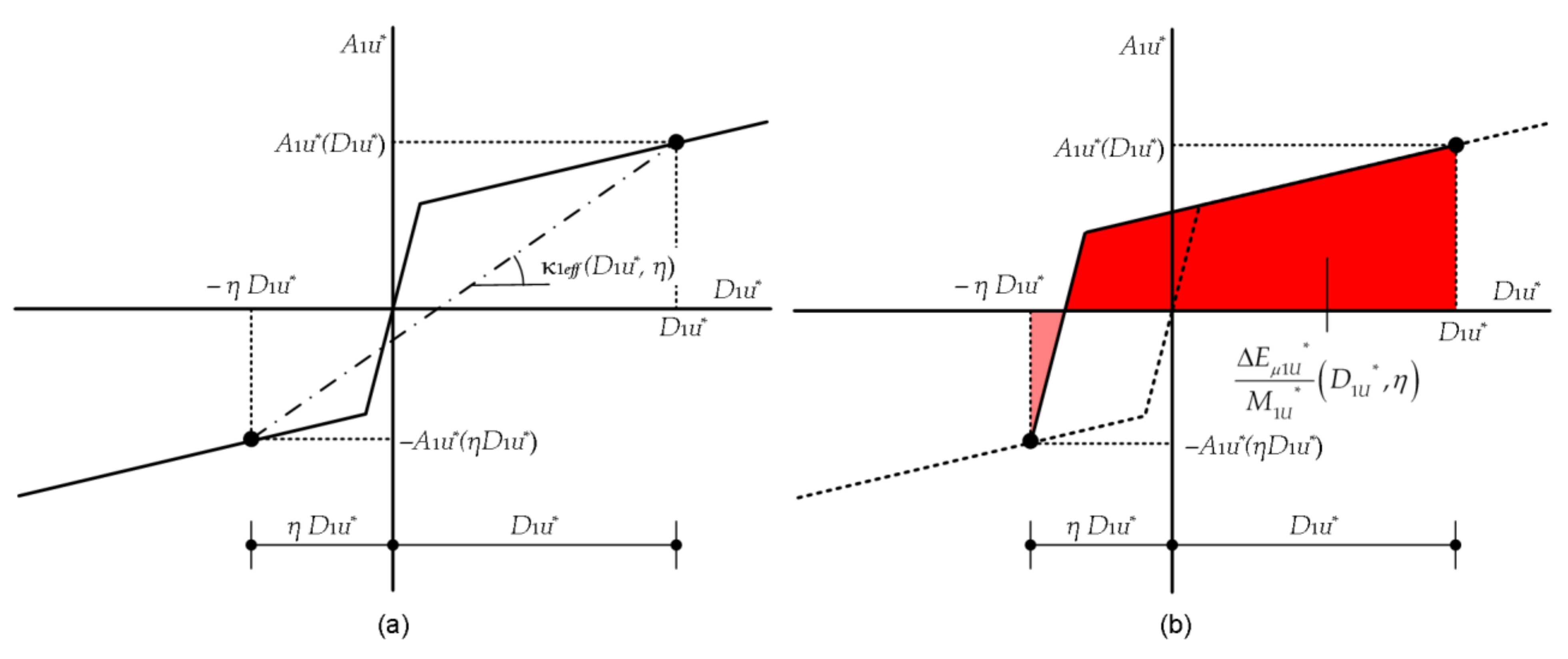
2.2.2. Formulation of the Effective Period and the Hysteretic Dissipated Energy in a Half Cycle
3. Description of the Retrofitted Building Models and Ground Motion Datasets
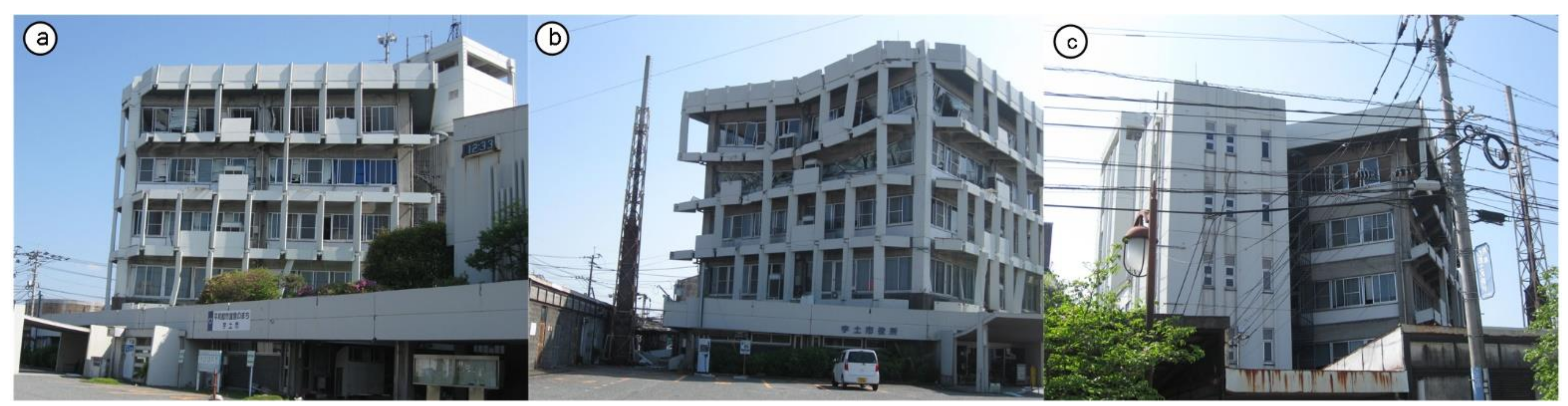
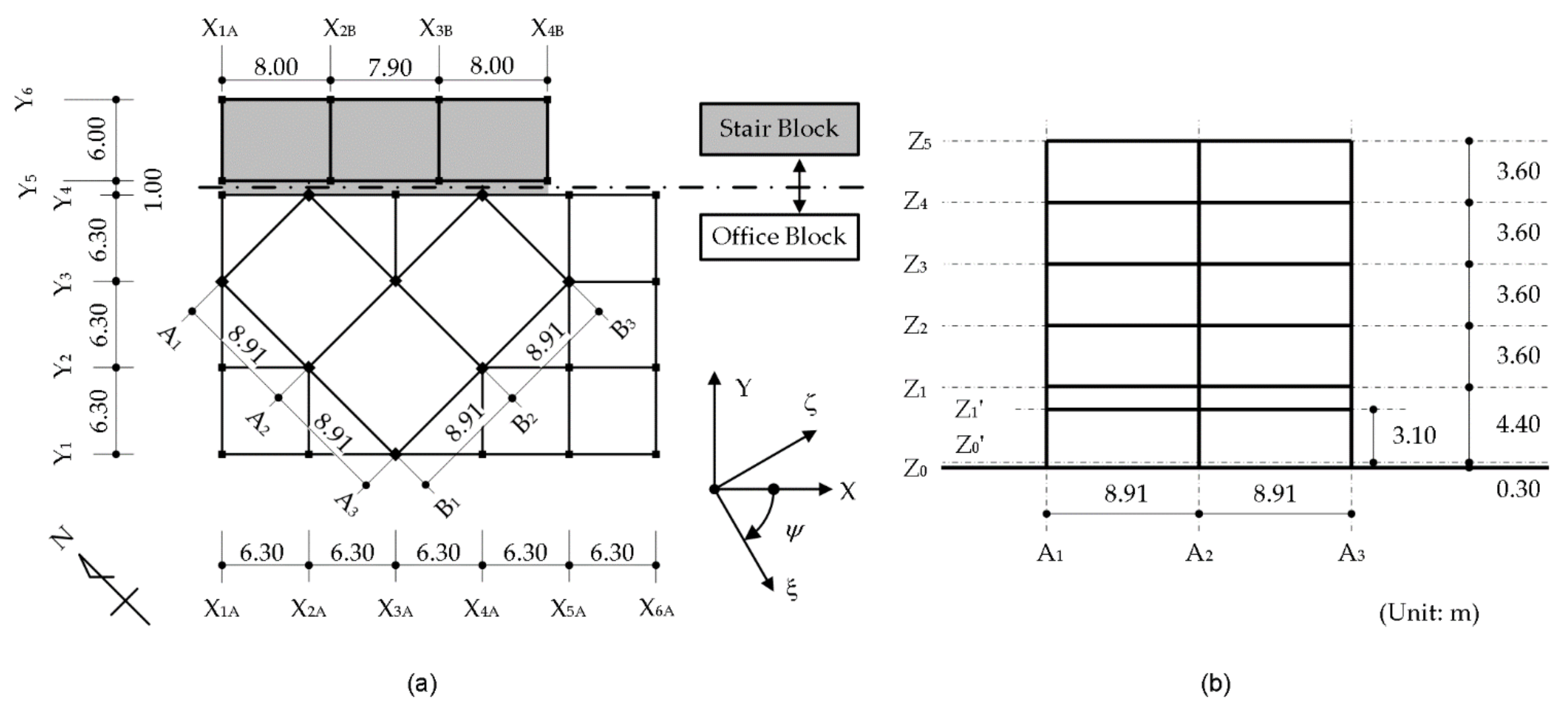
3.1. Original Building
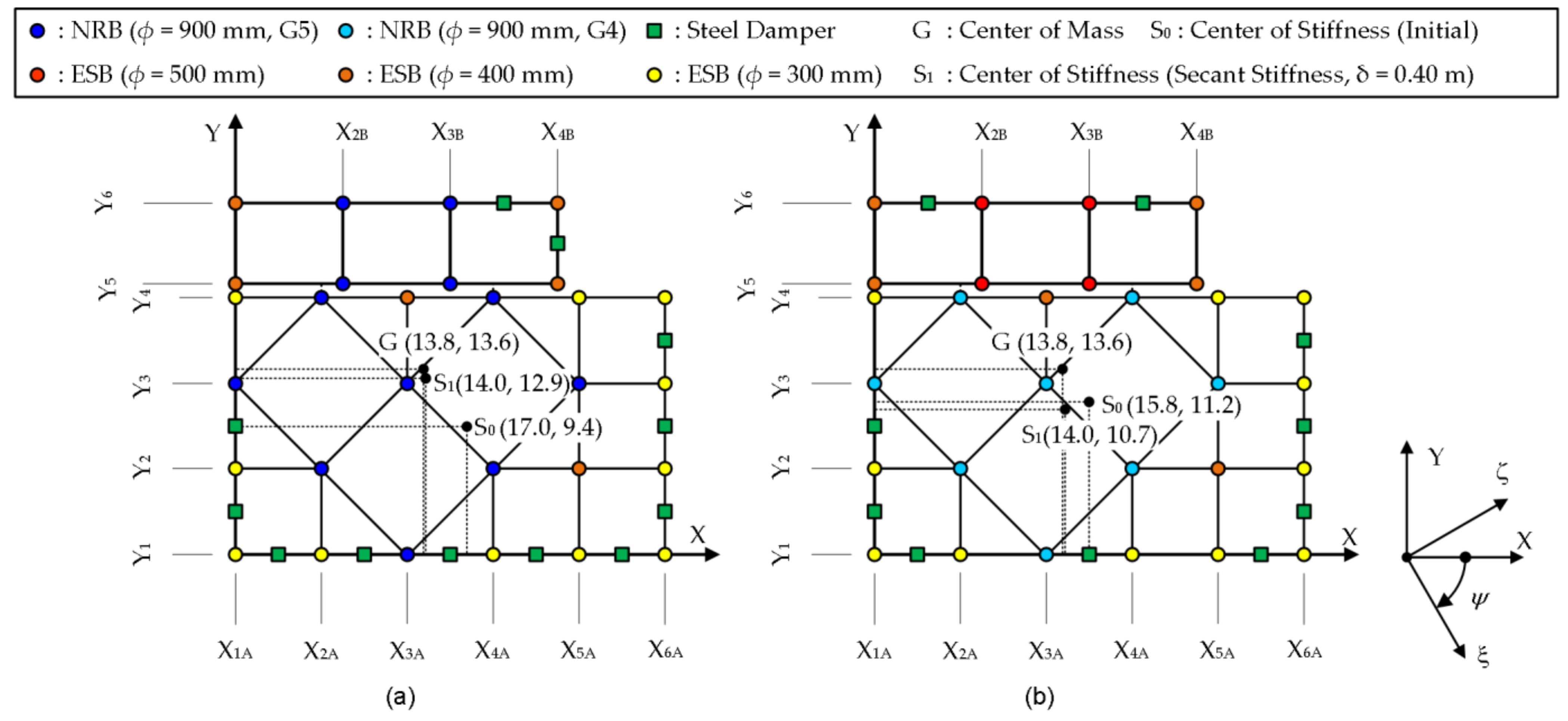
3.2. Properties of the Isolation Layer
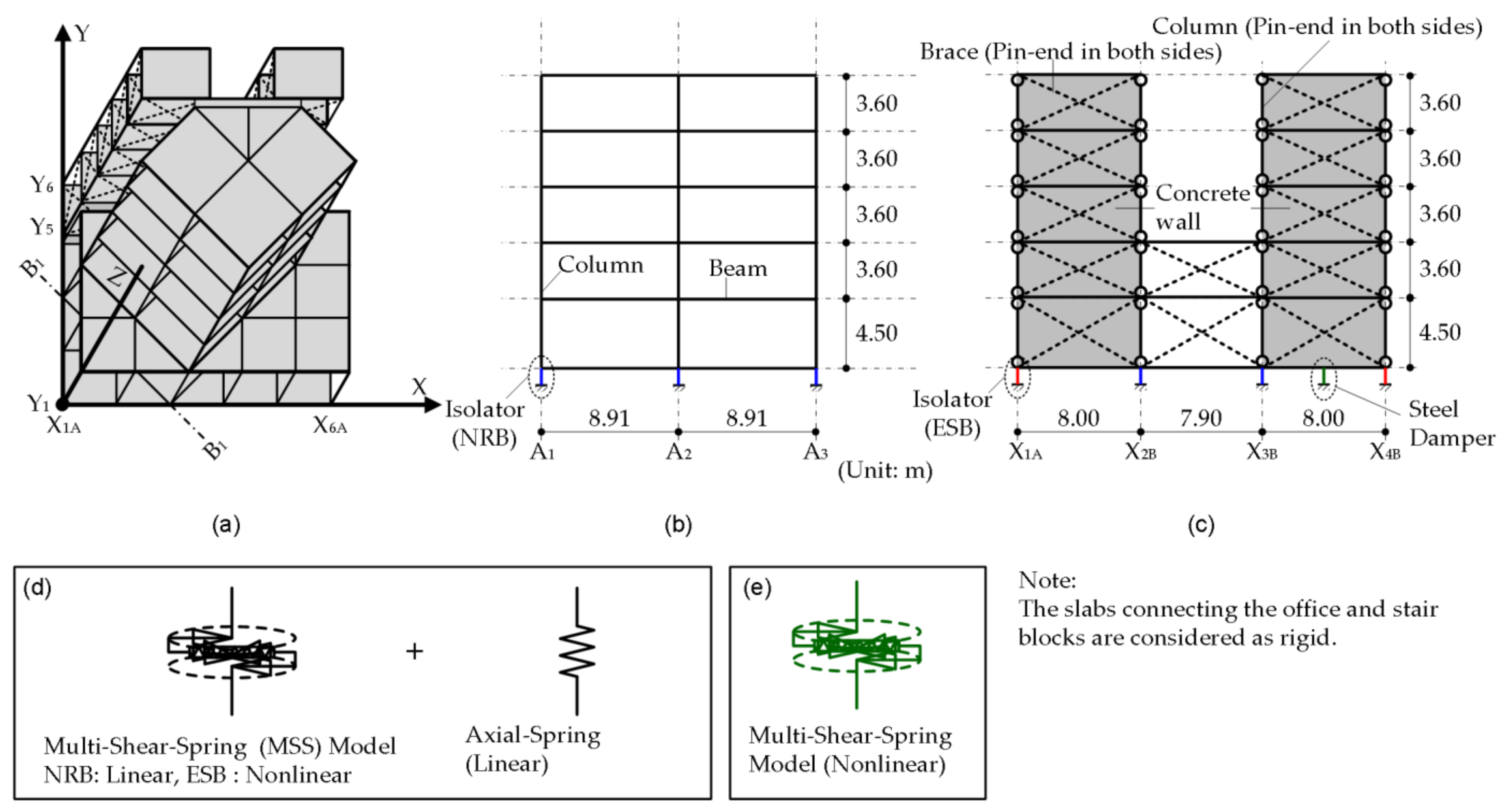
3.3. Structural Modeling
3.4. Ground Motion Data
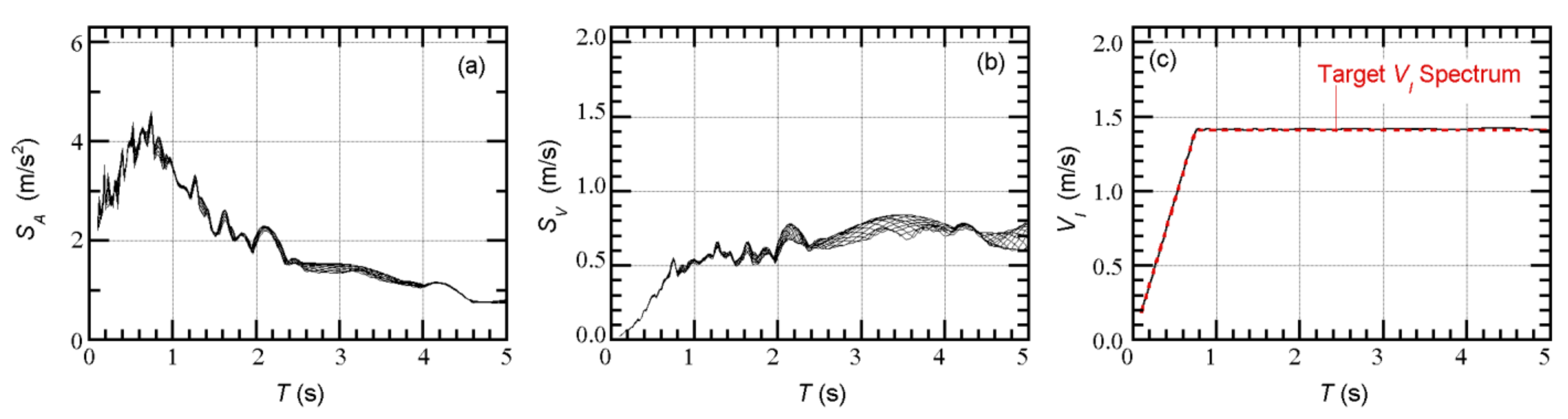
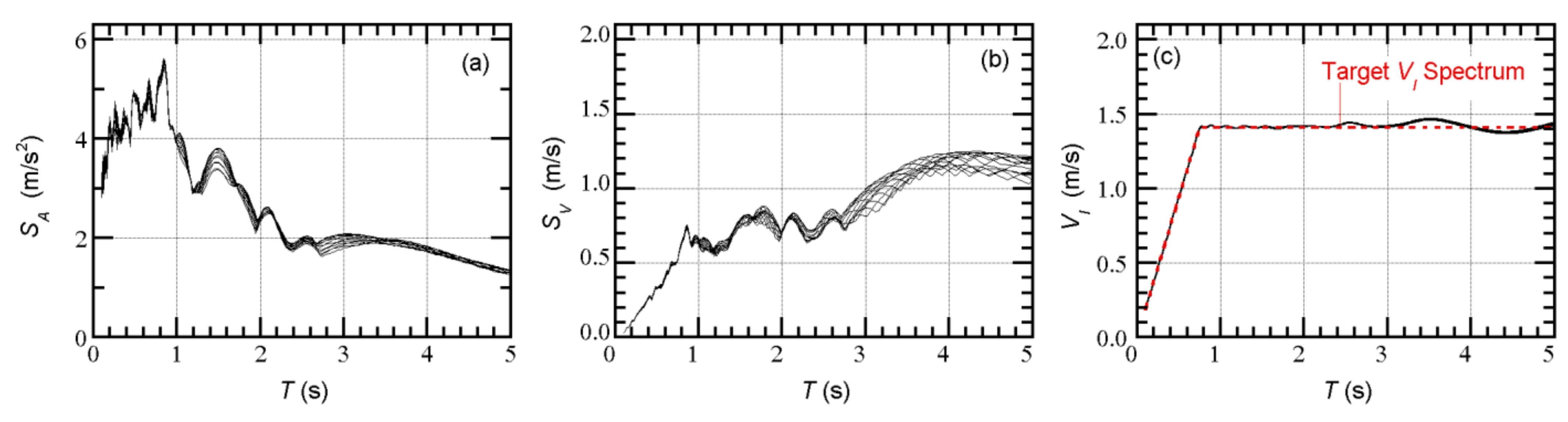
3.4.1. Artificial Ground Motions
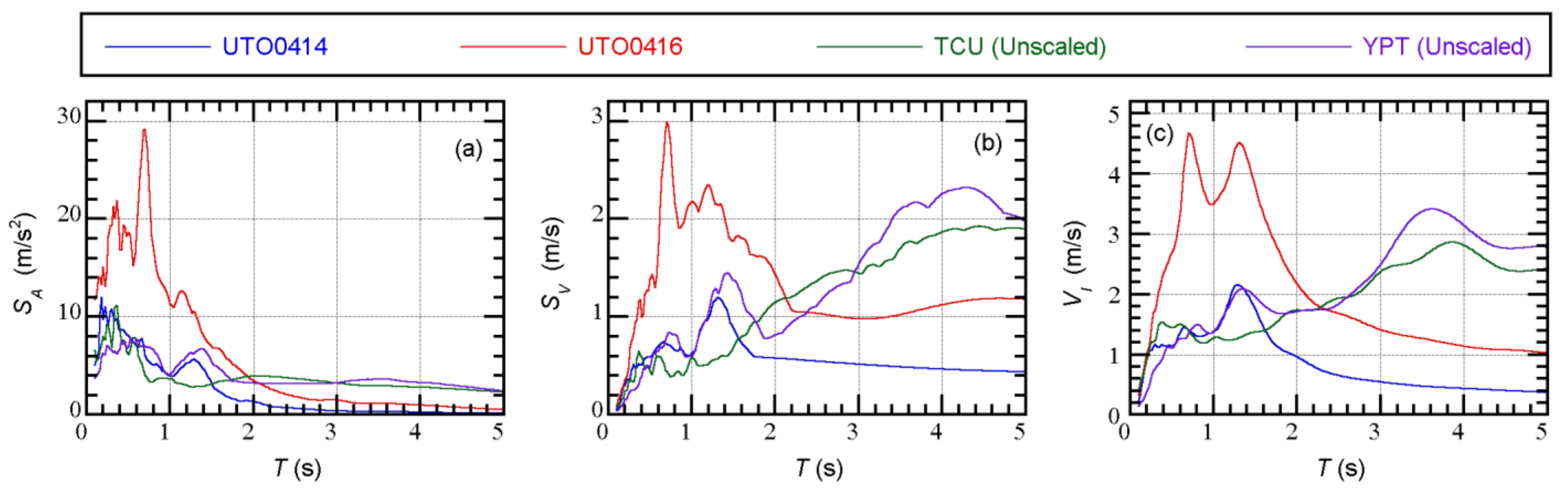
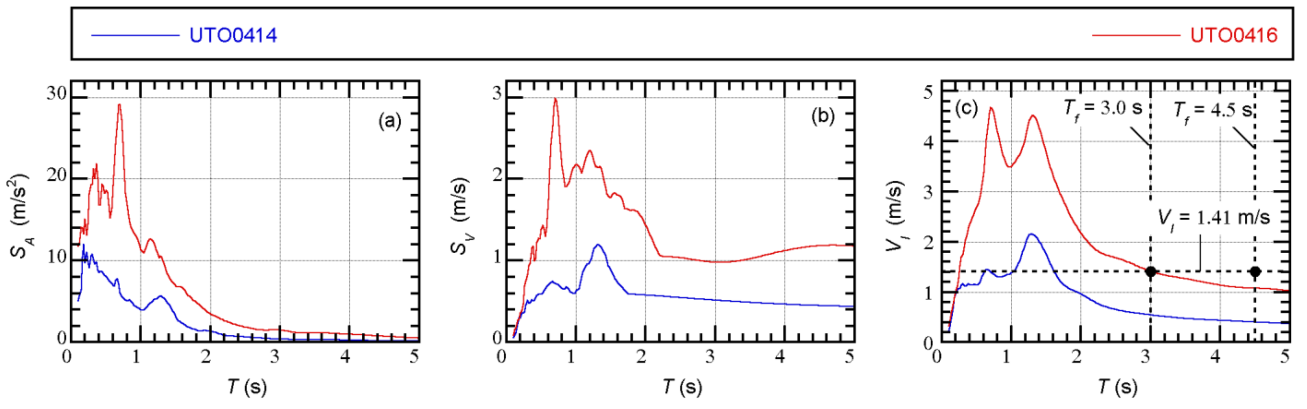
3.4.2. Recorded Ground Motions
4. Analysis Results
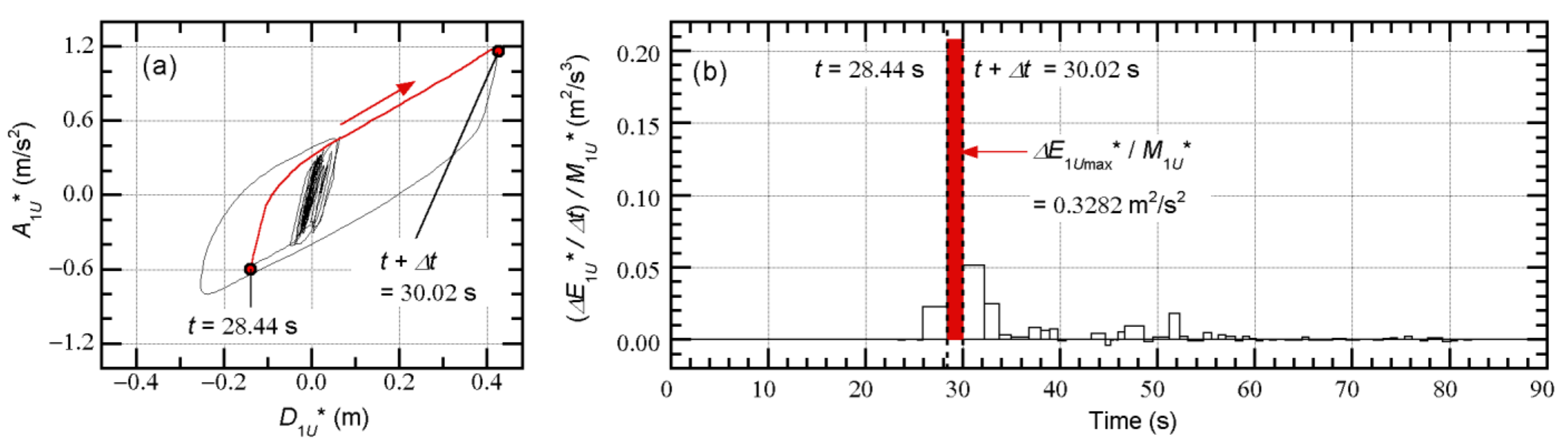
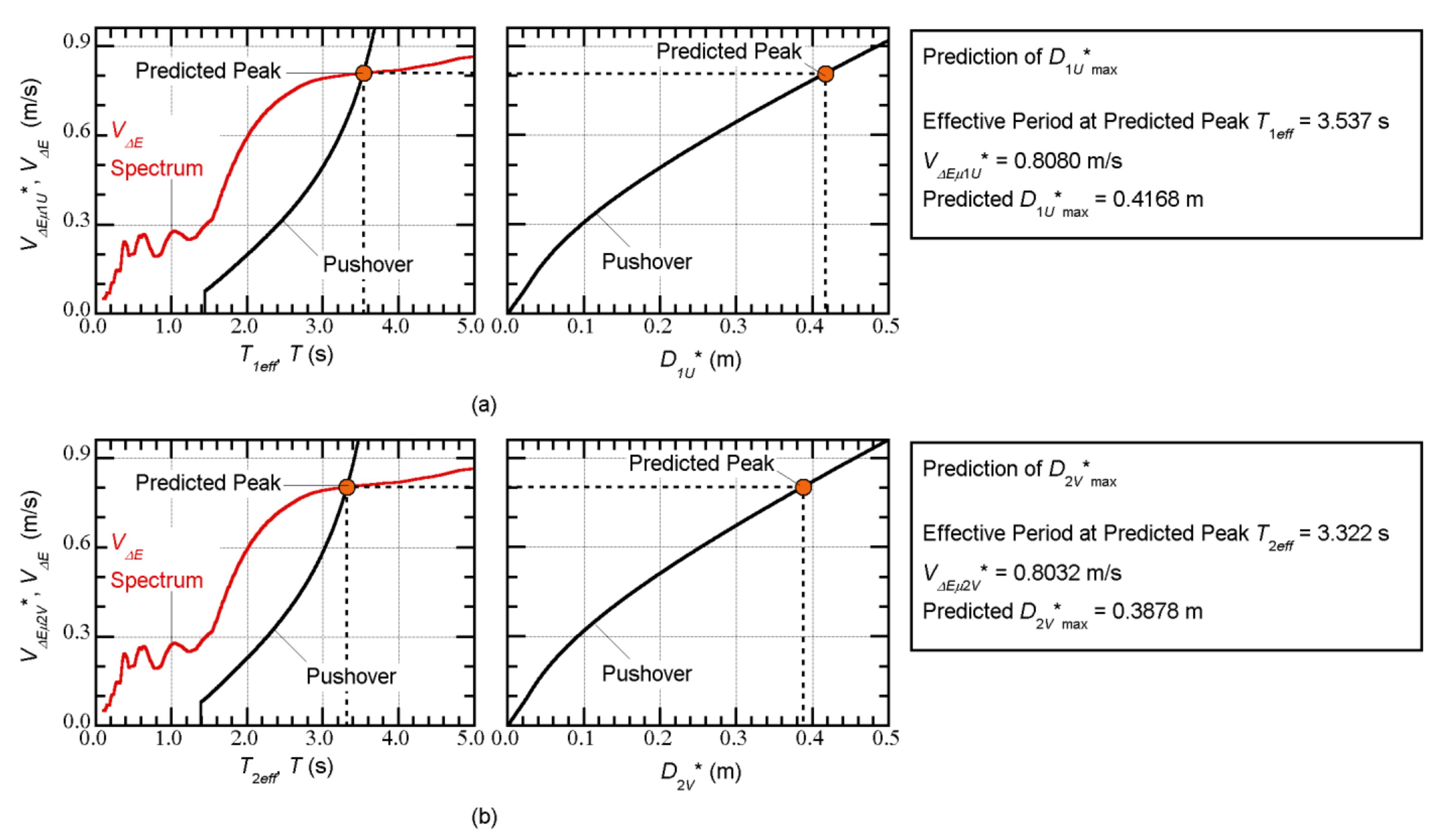
4.1. Example of a Prediction of the Peak Equivalent Displacement
4.2. Comparisons with the Nonlinear Time-History Analysis
4.2.1. Artificial Ground Motion
4.2.2. Recorded Ground Motion
5. Discussion
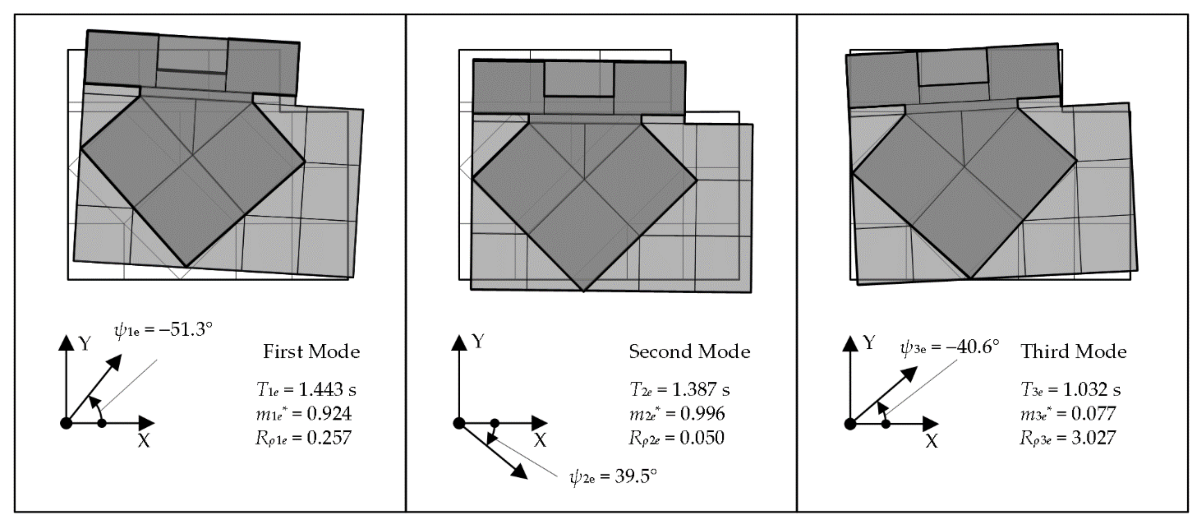
5.1. Calculation of the Modal Responses
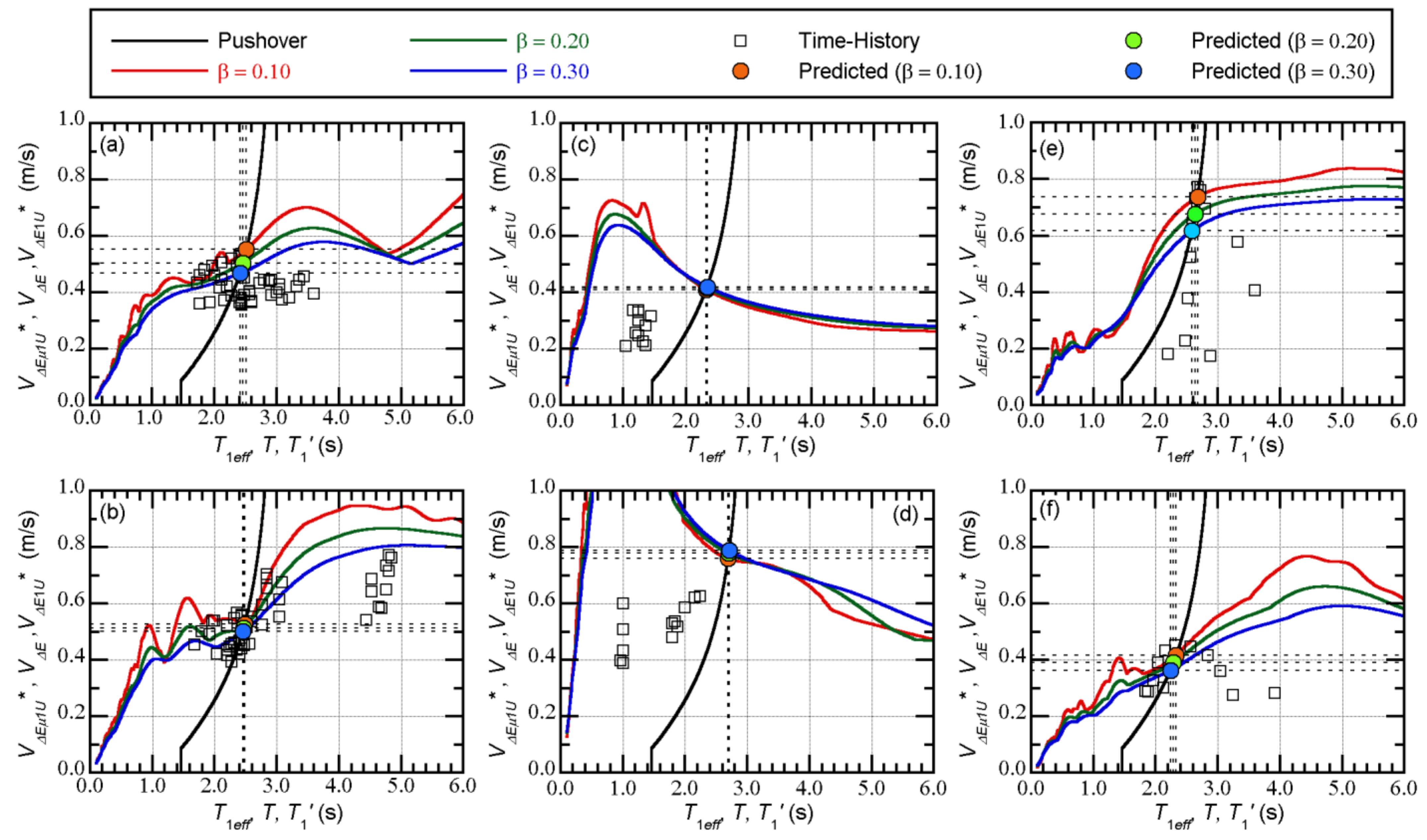
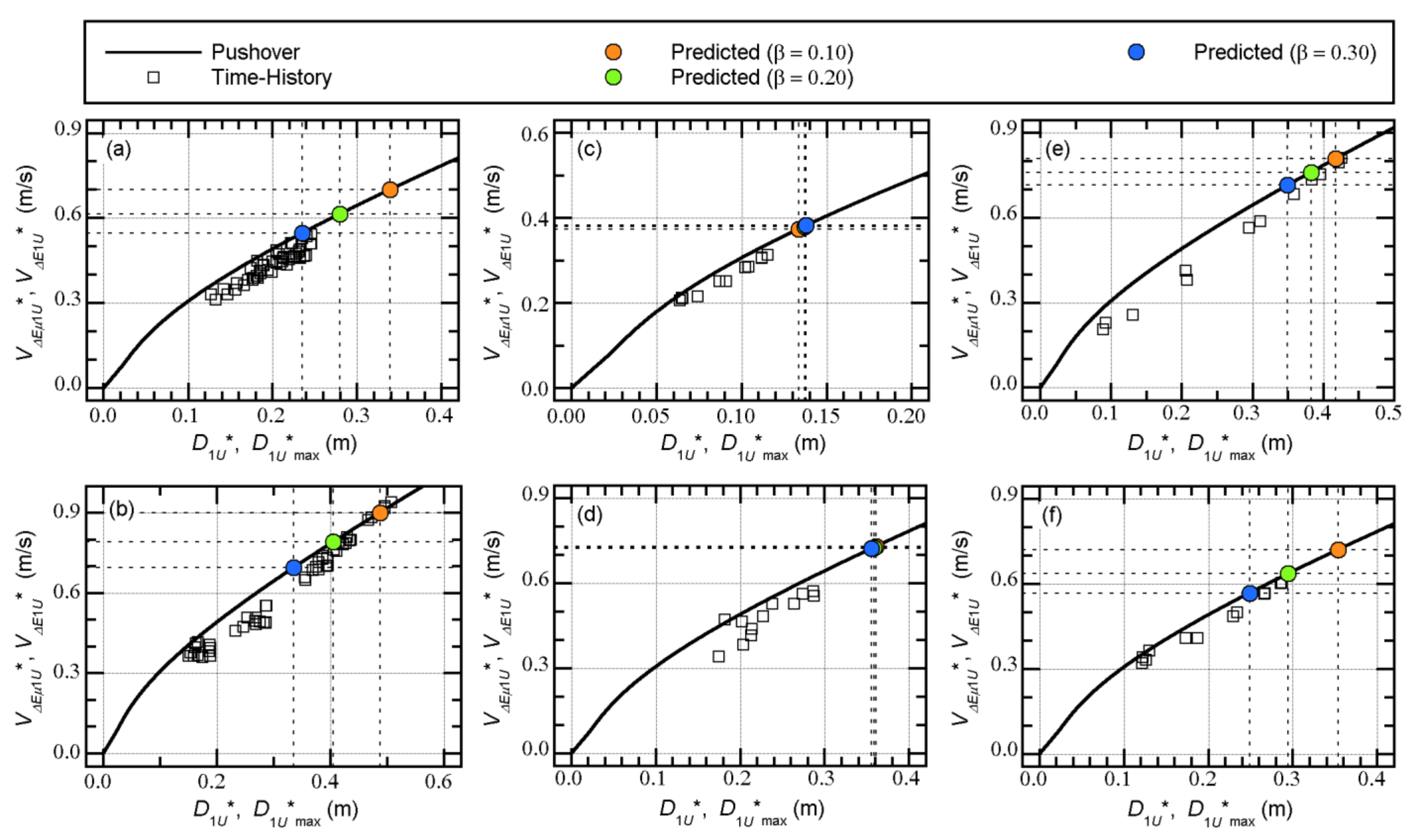
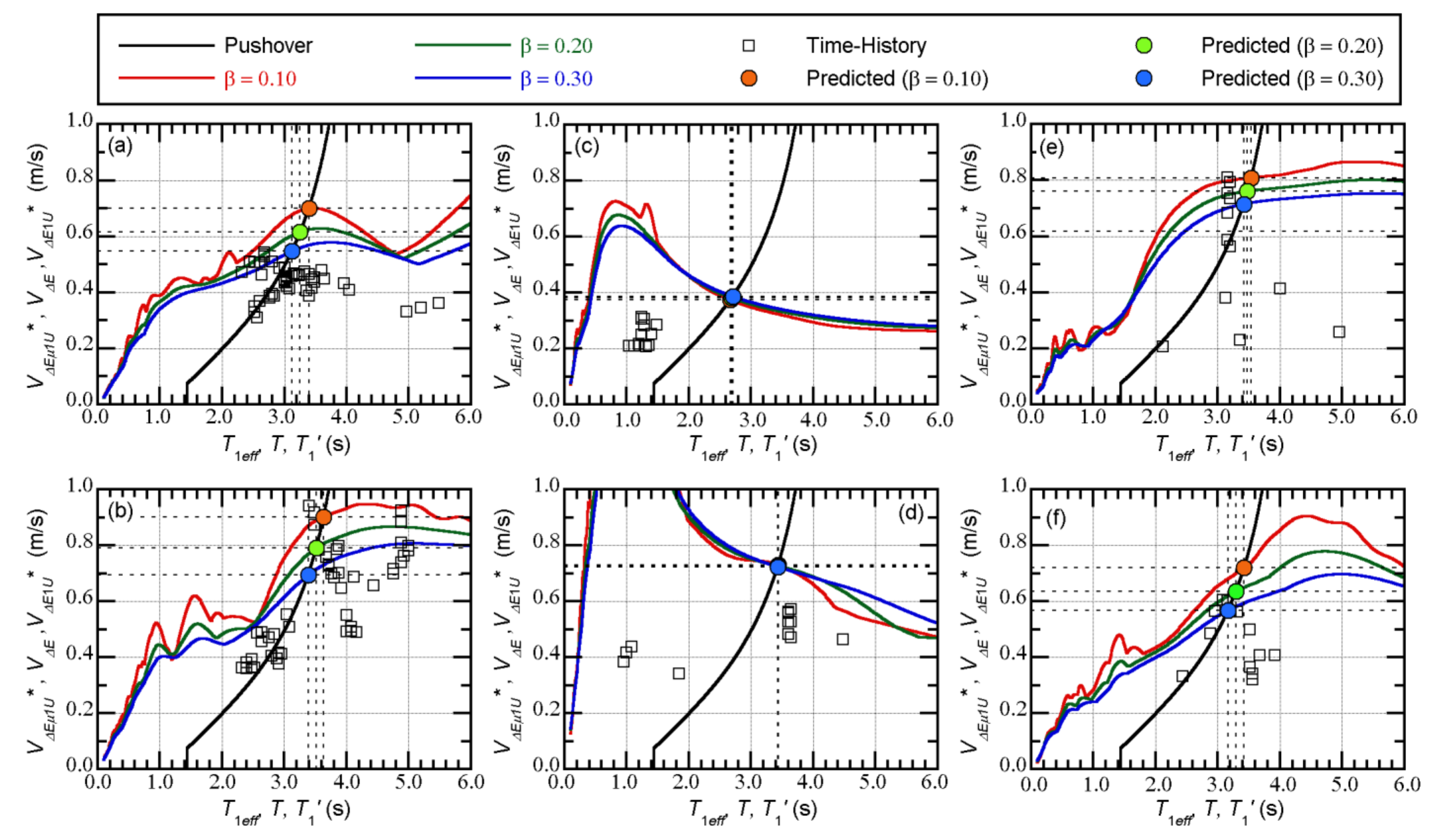
5.2. Relationship between the Peak Equivalent Displacement and the Maximum Momentary Input Energy of the First Modal Response
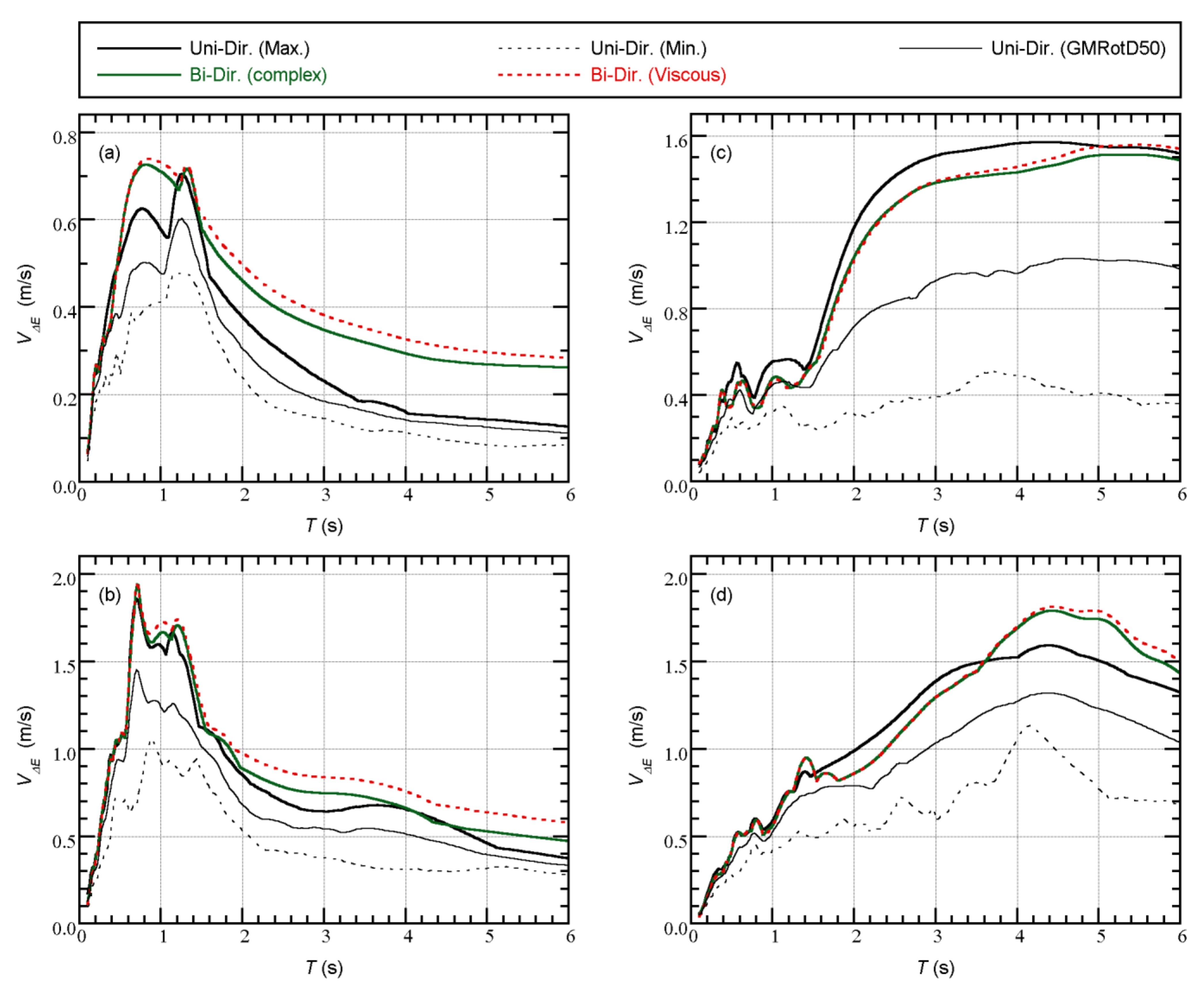
5.3. Comparison of the Maximum Momentary Input Energy and the Bidirectional Momentary Input Energy Spectrum
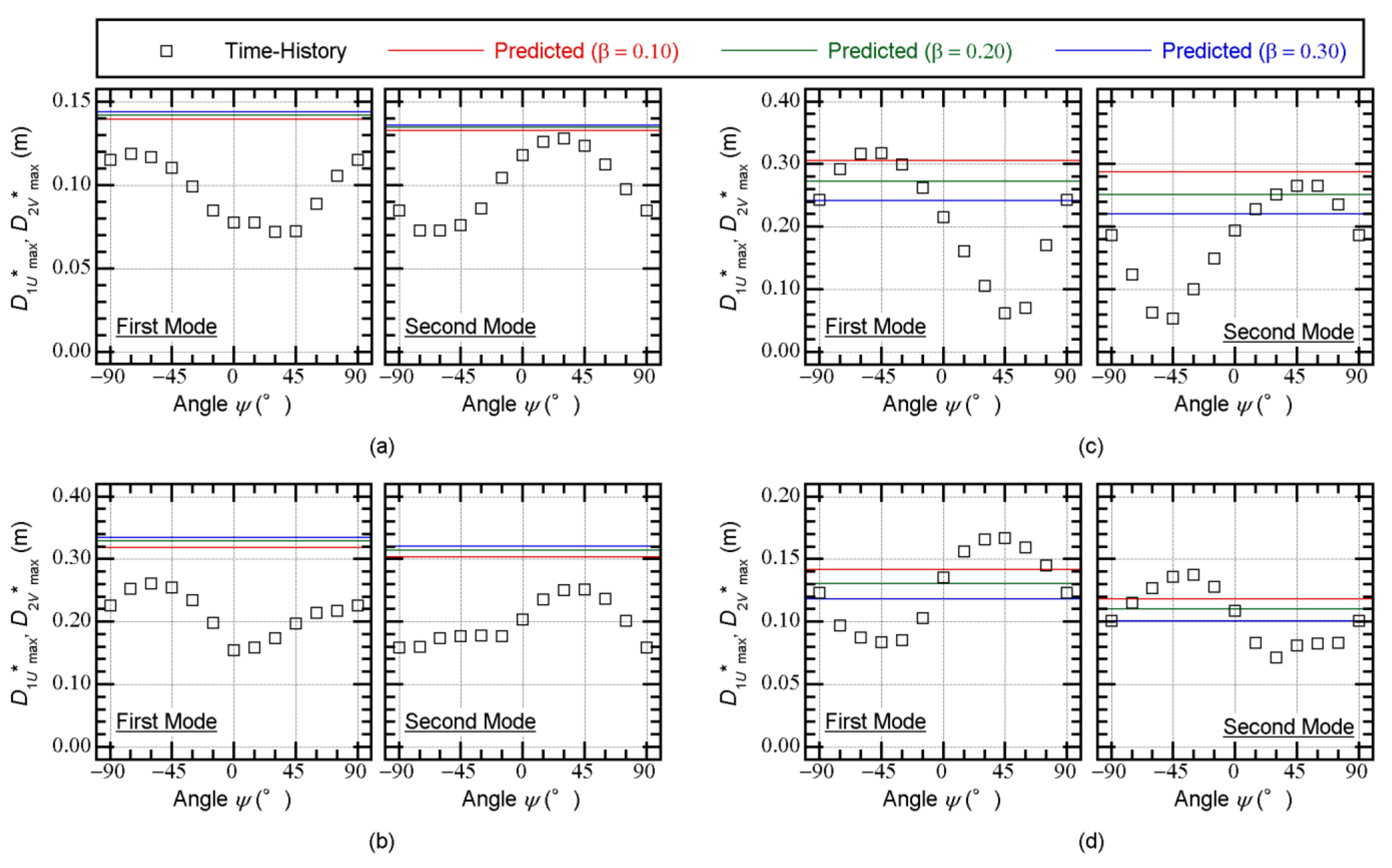
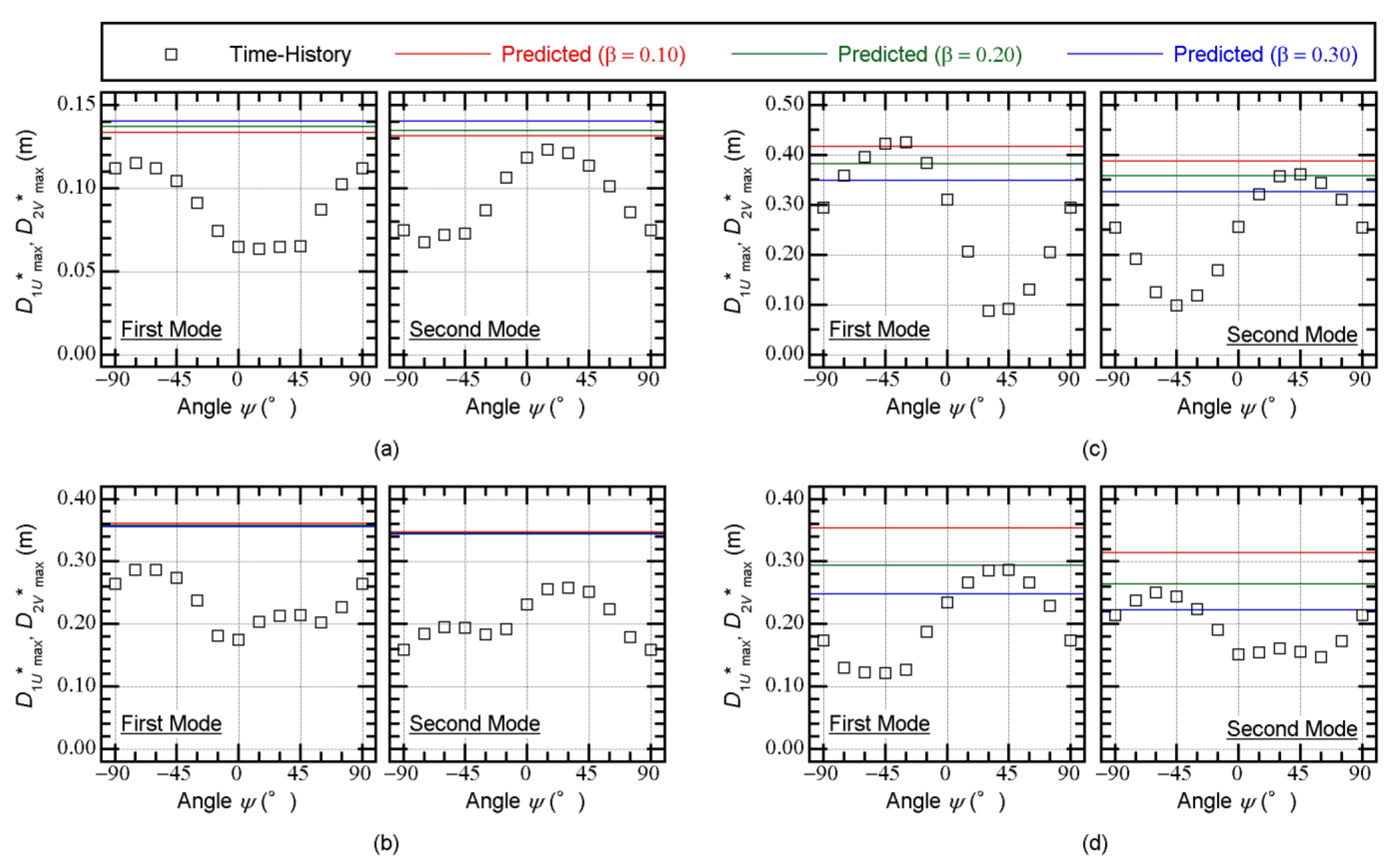
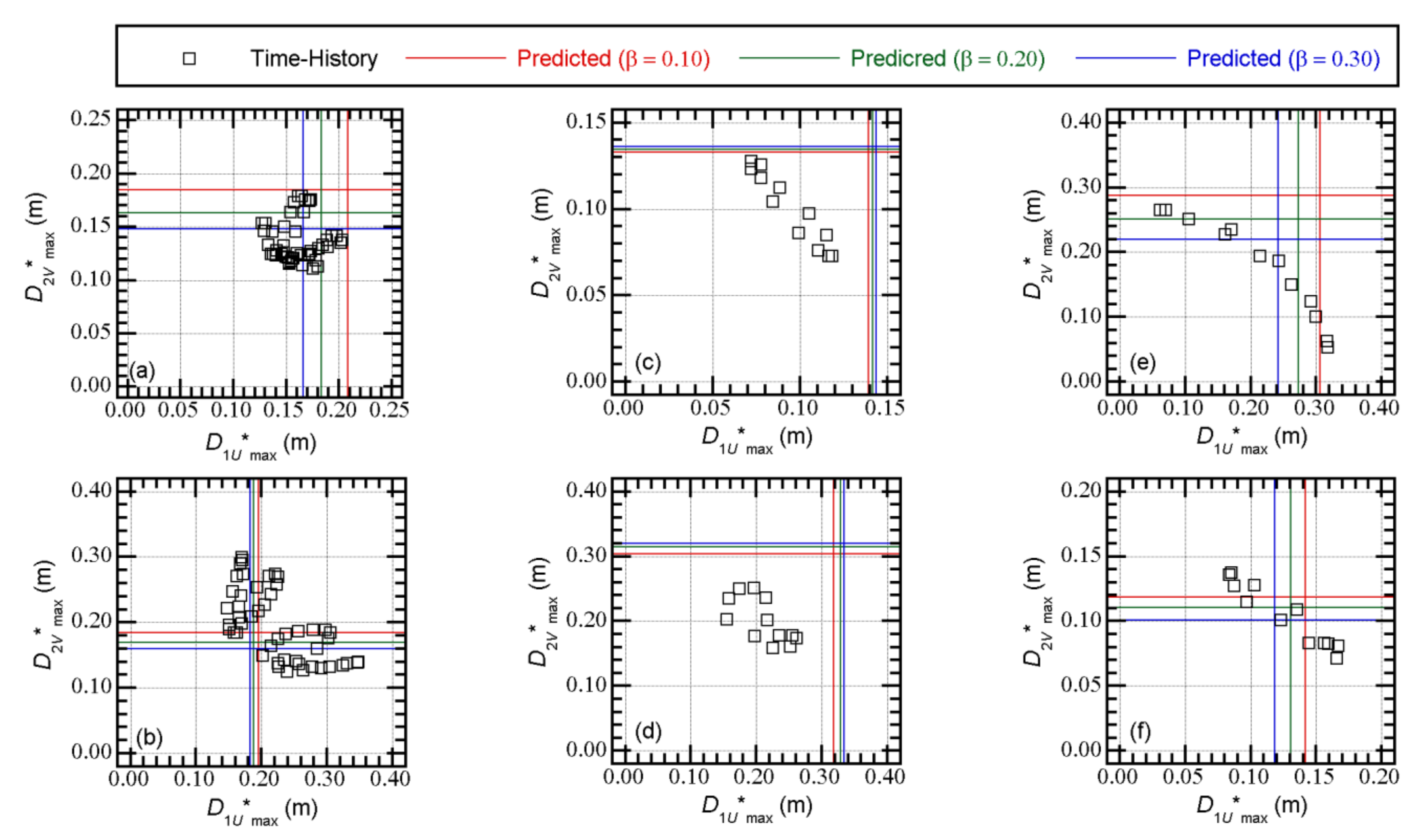
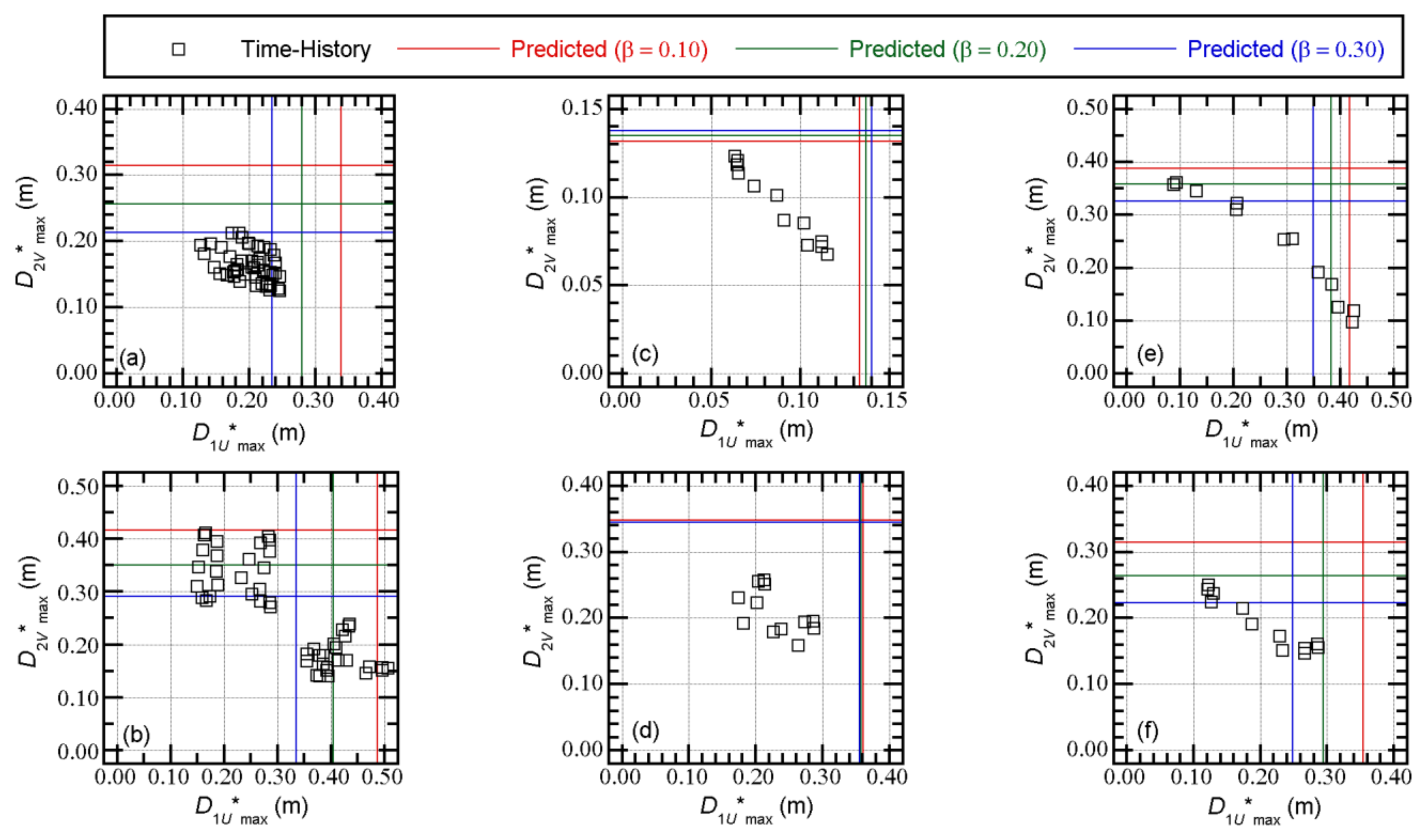
5.4. Accuracy of the Predicted Peak Equivalent Displacements of the First and Second Modal Responses
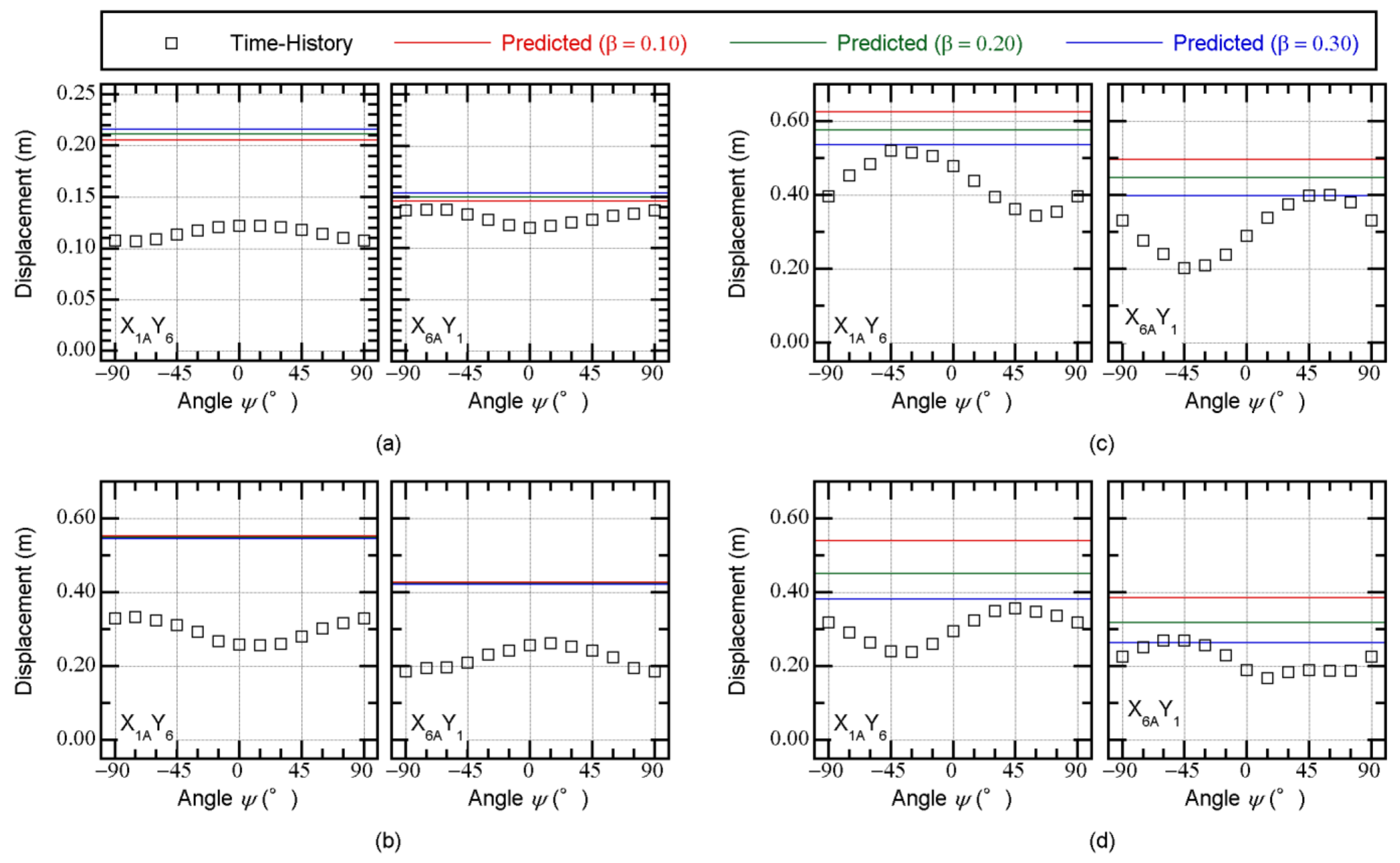
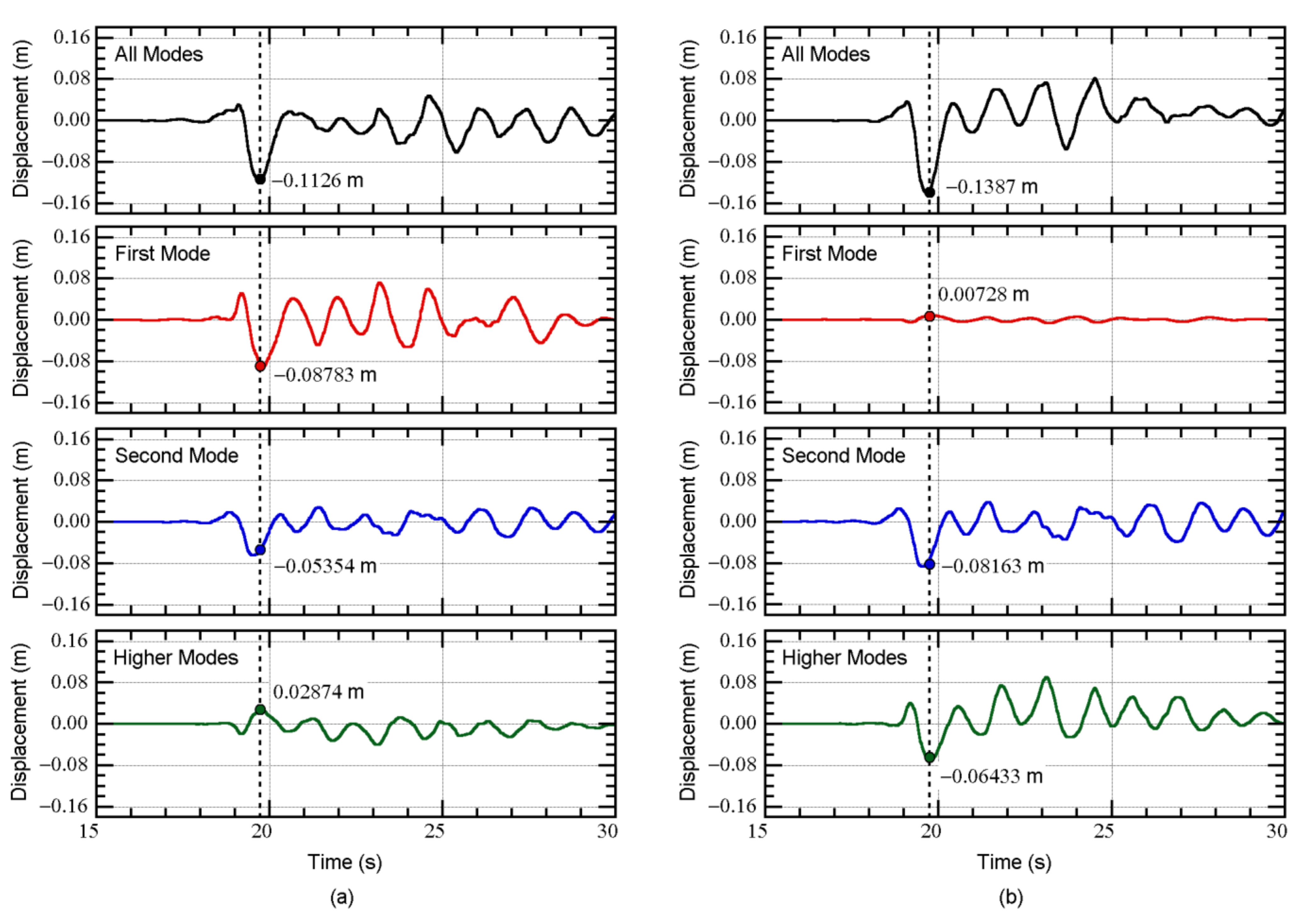
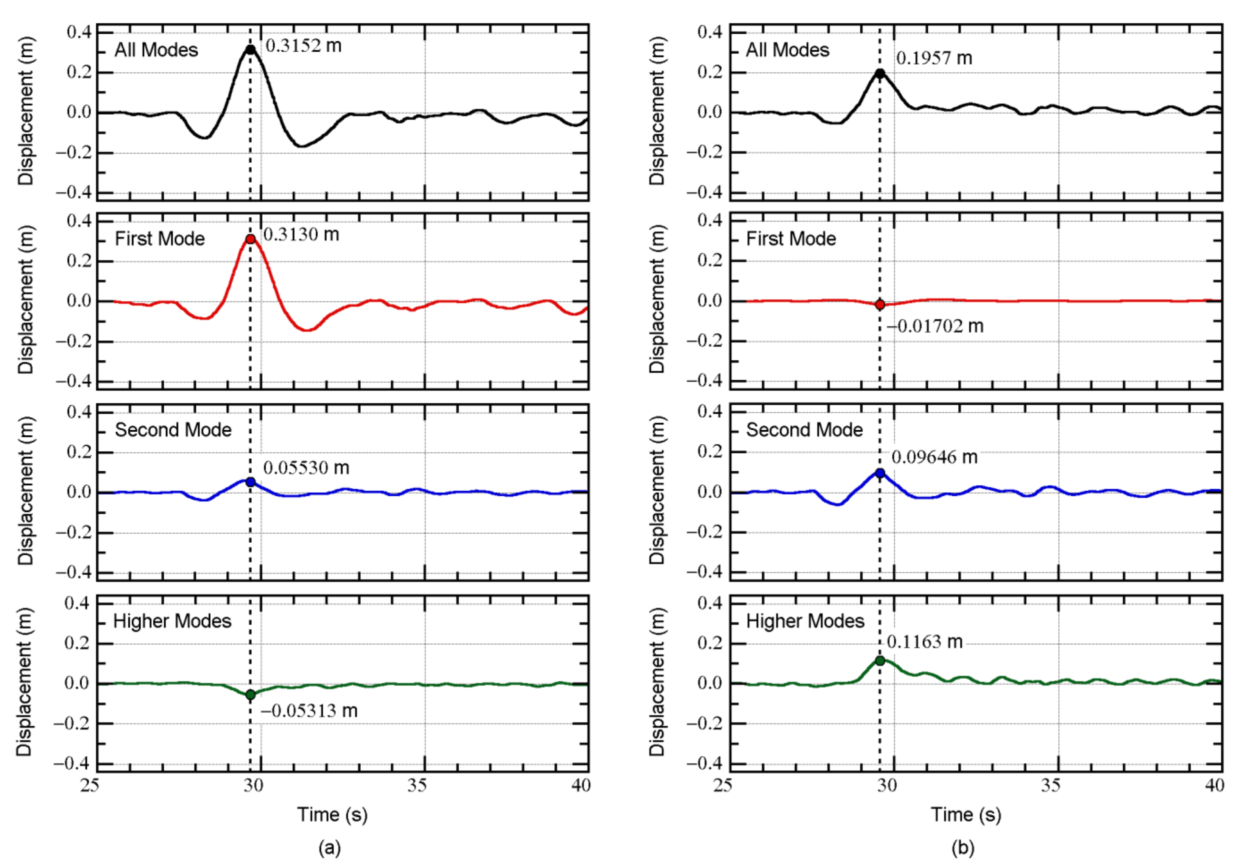
5.5. Contribution of the Higher Mode to the Displacement Response at the Edge of Level 0
5.6. Summary of the Discussions
6. Conclusions
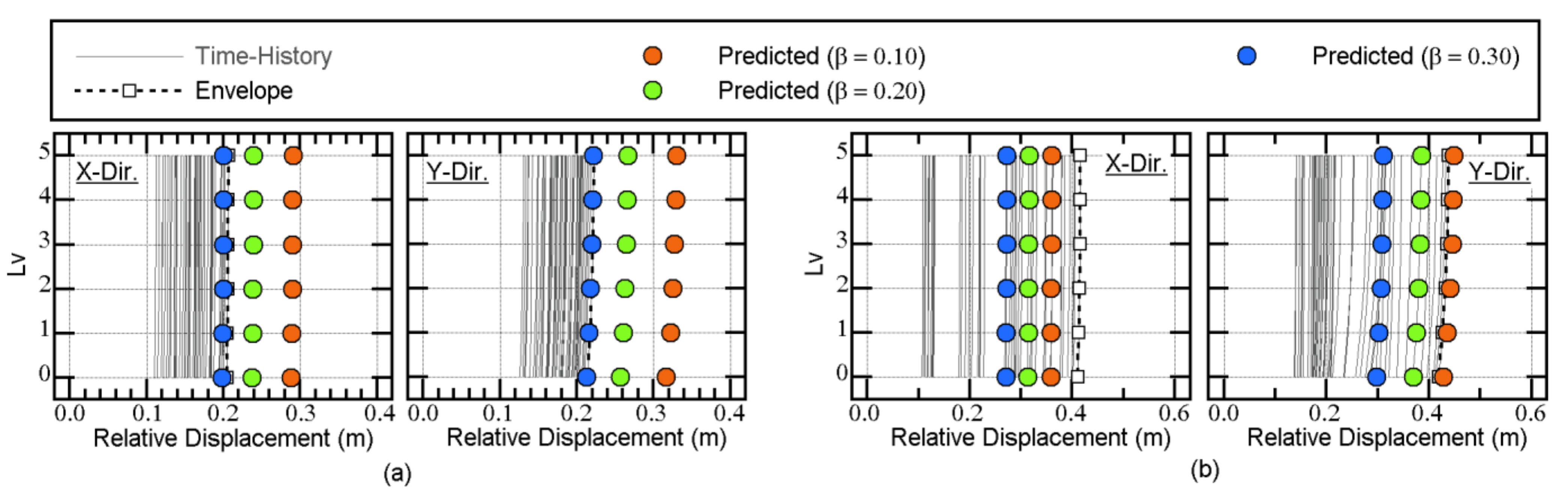
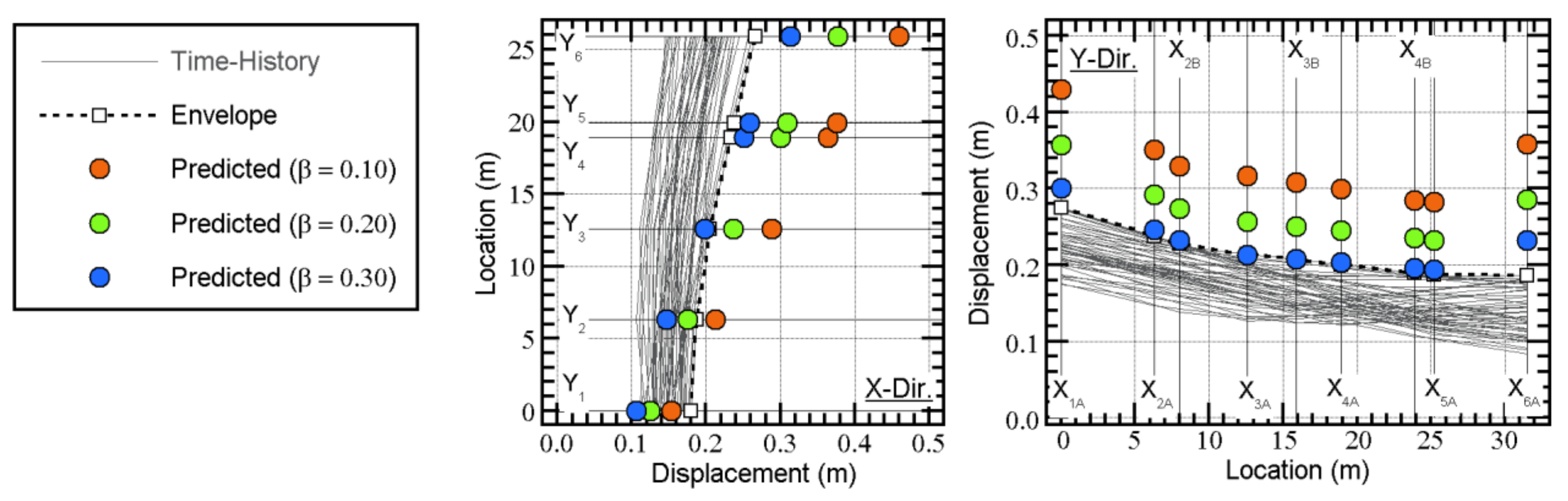
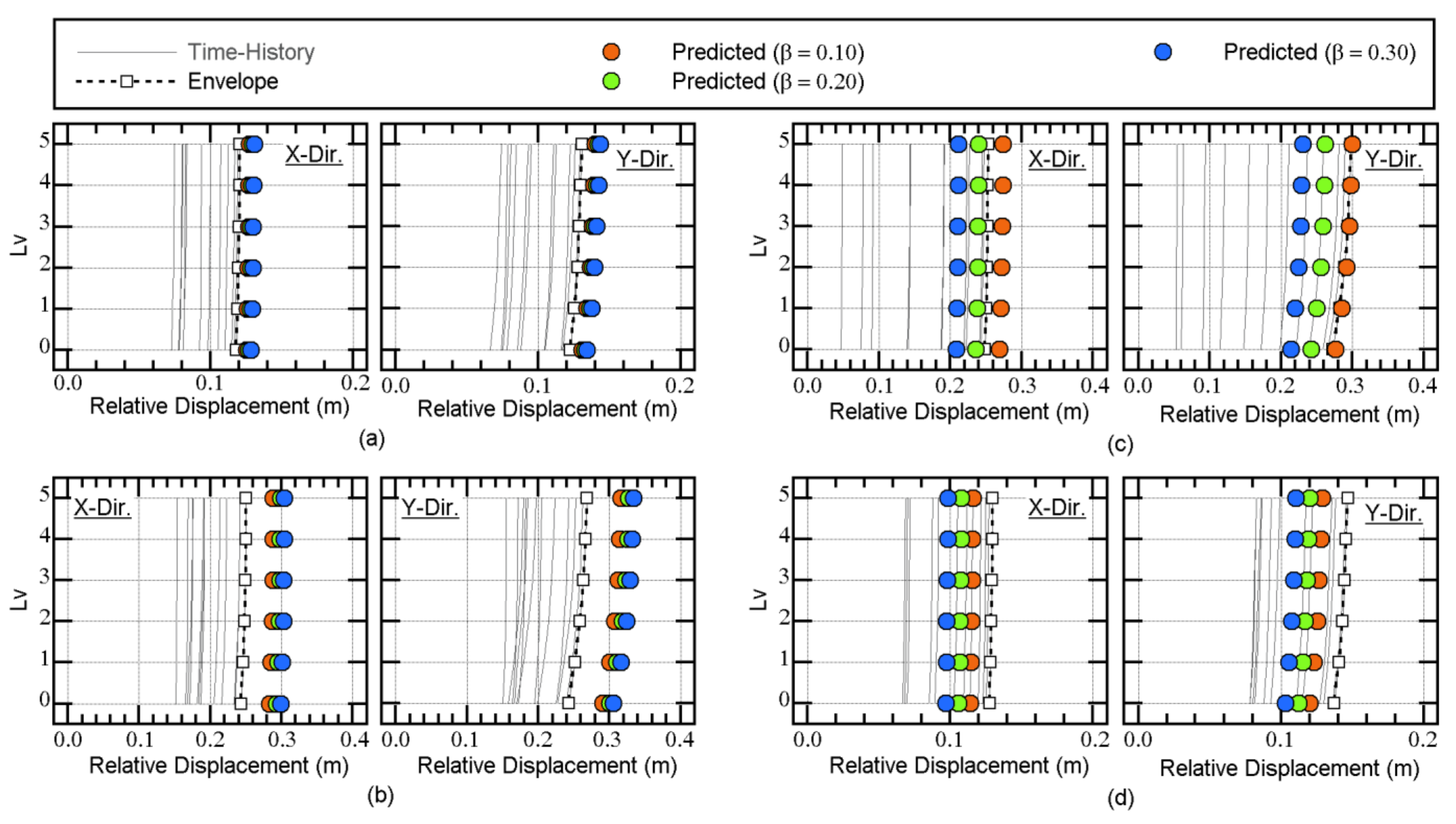
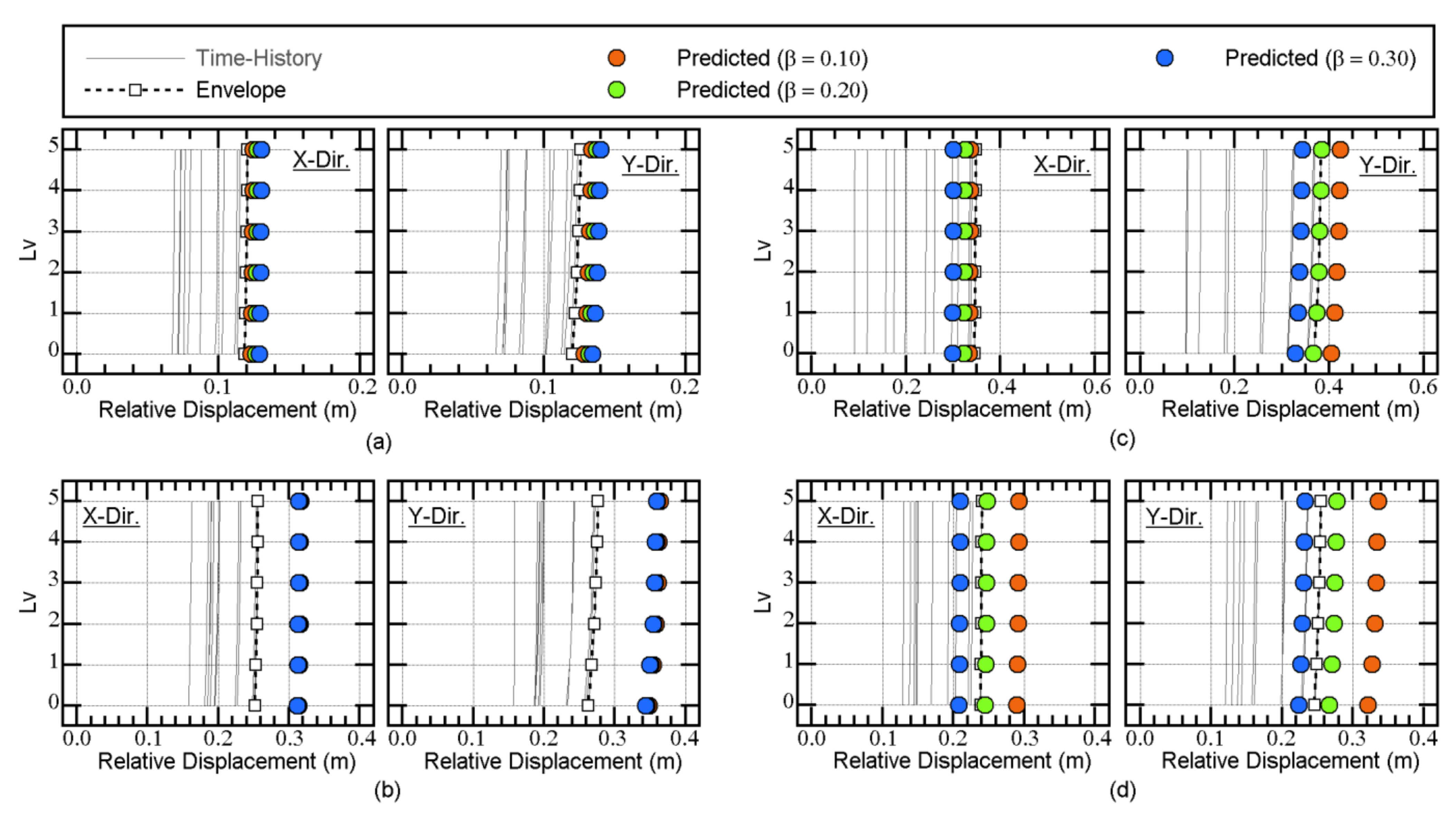
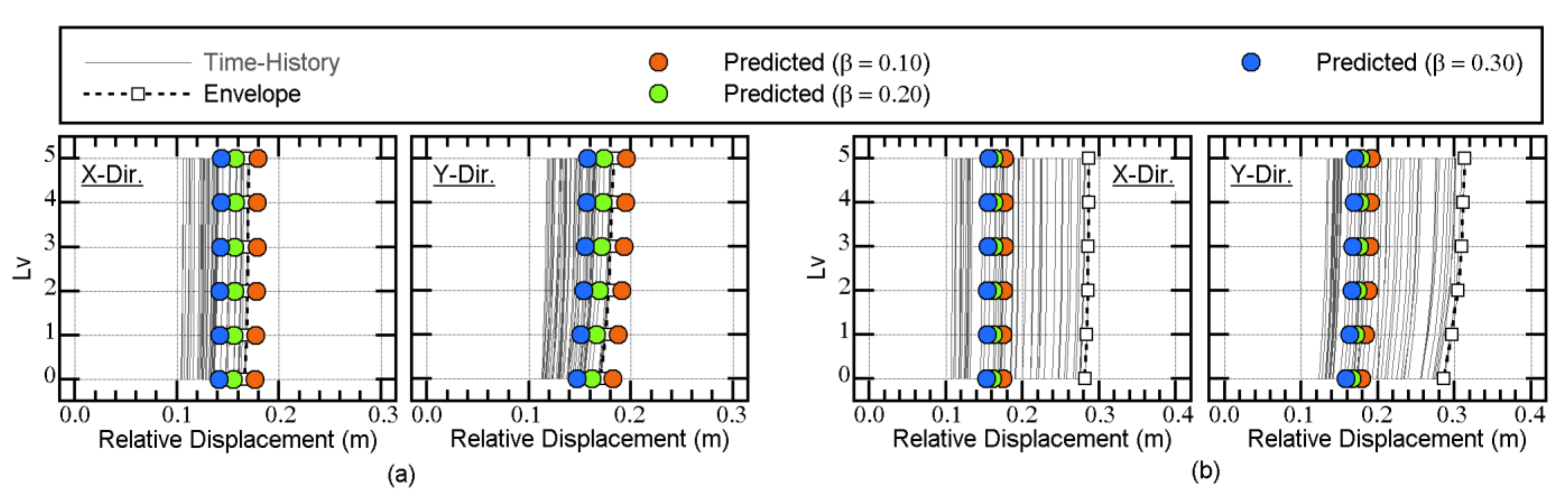
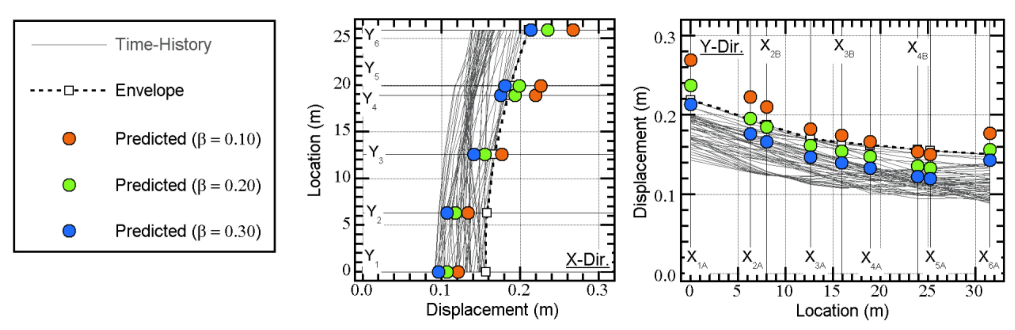
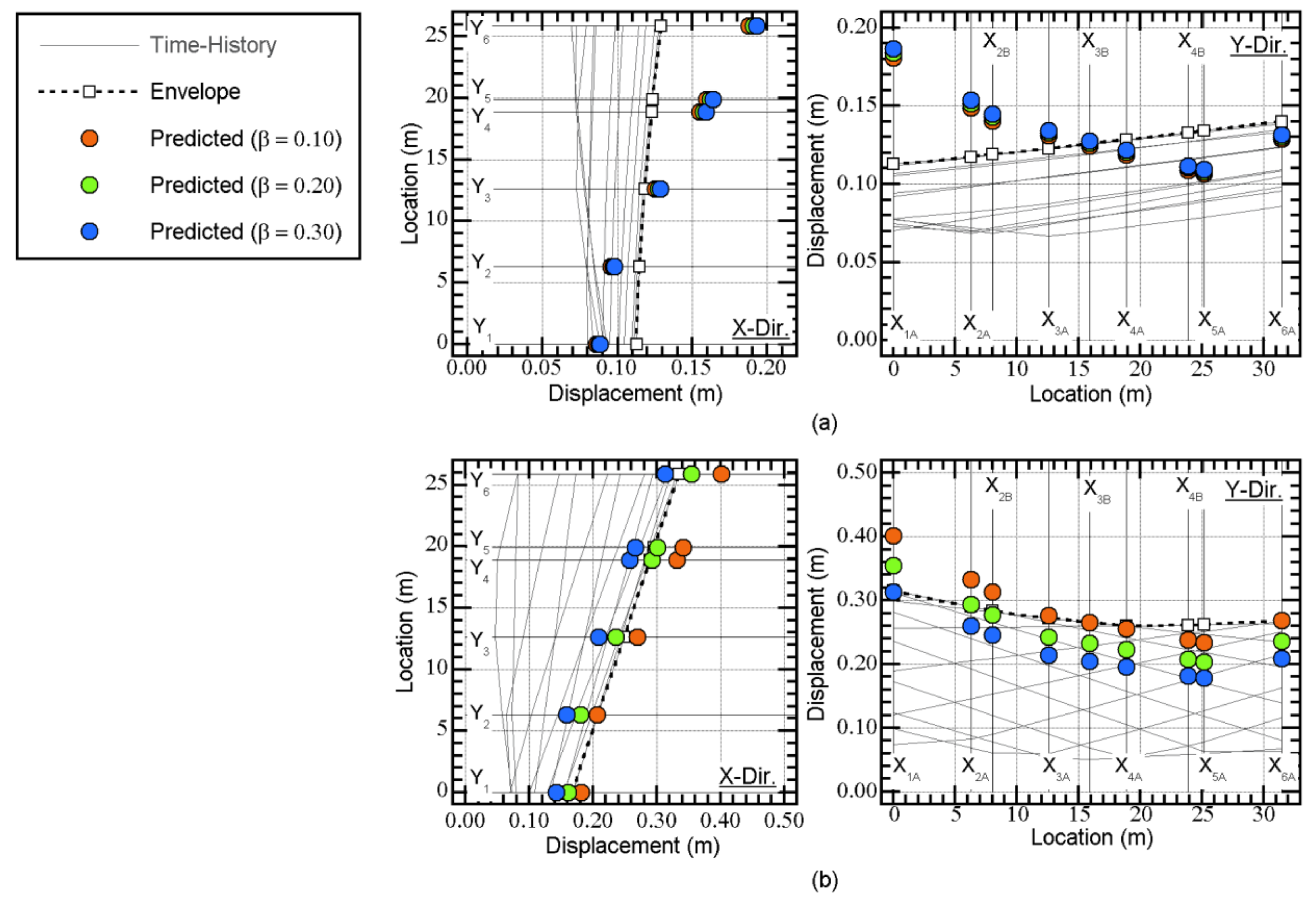
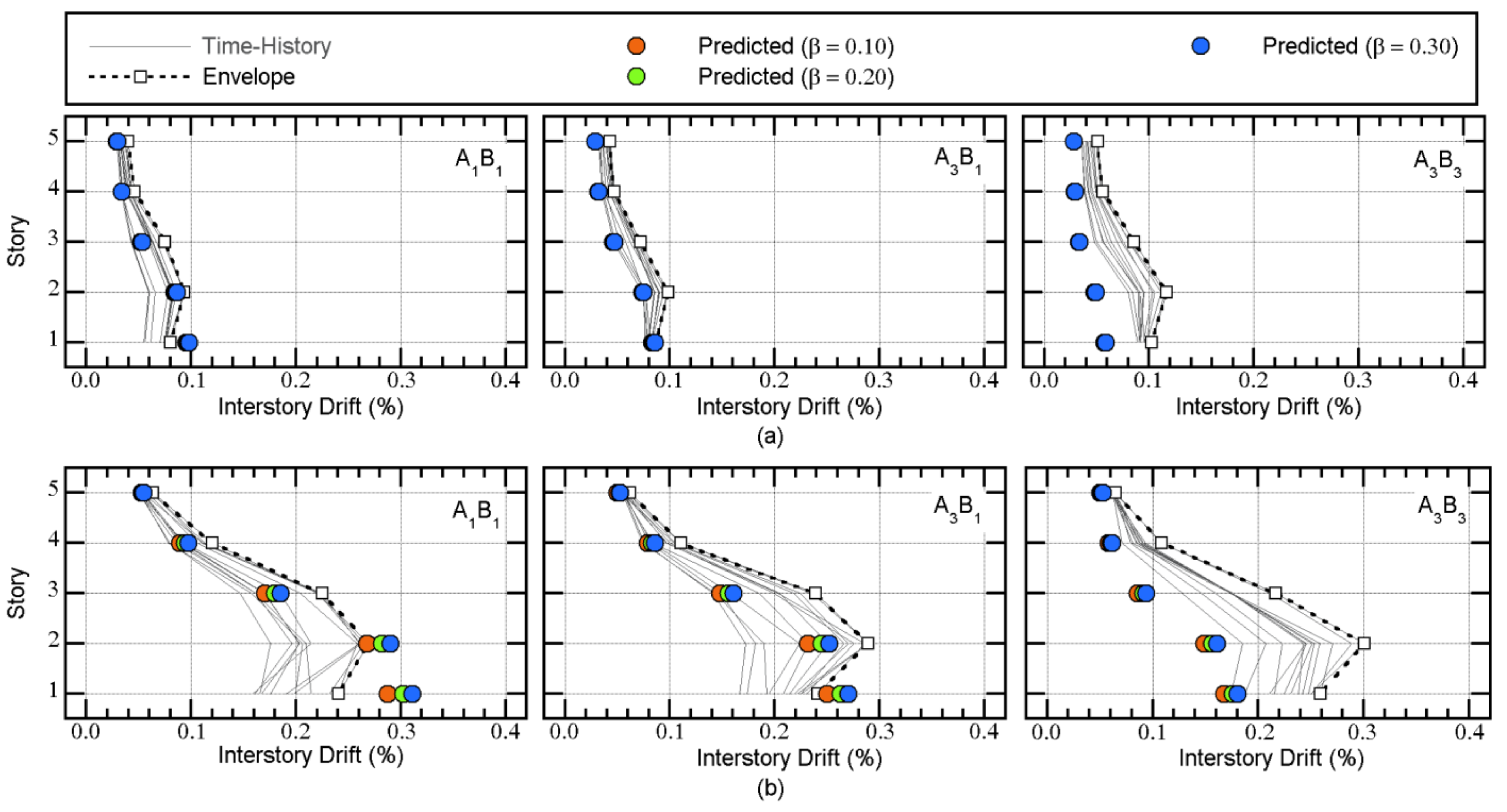
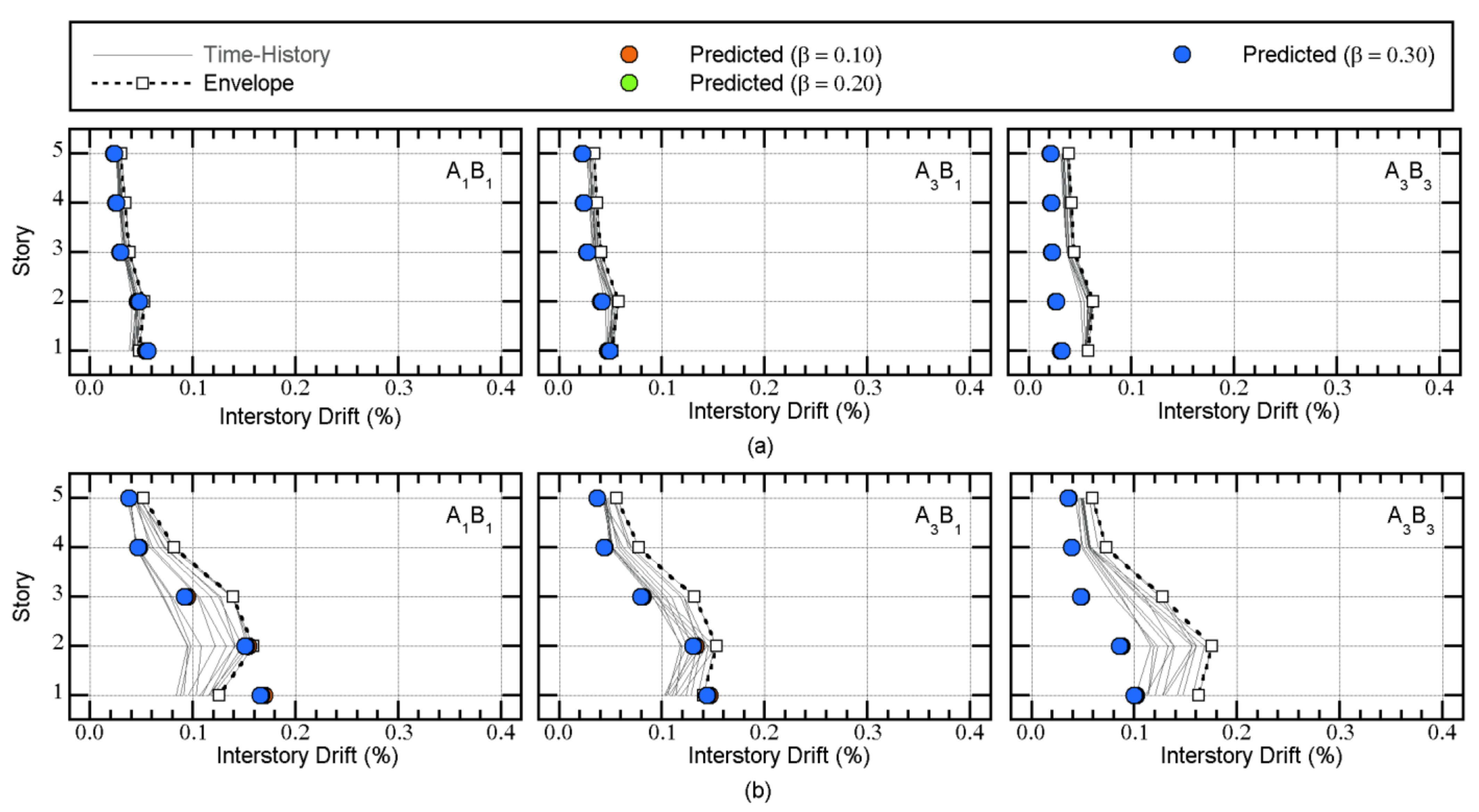
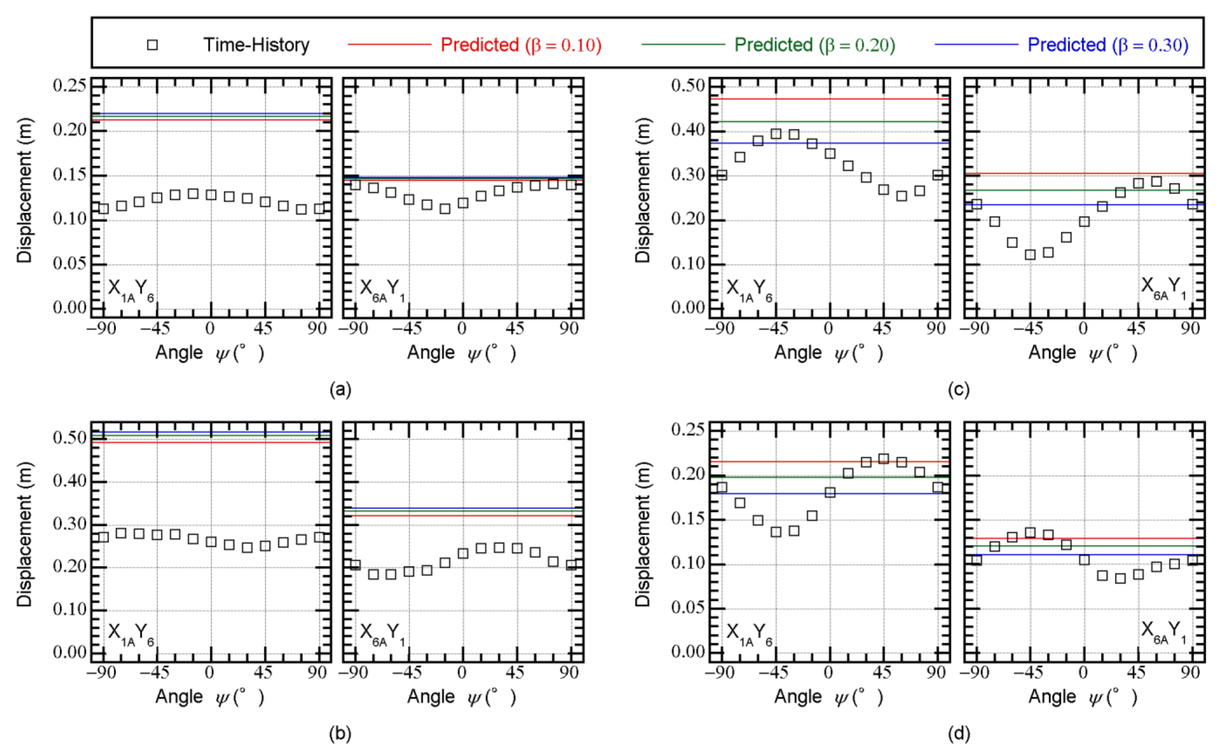
- The predicted peak response according to the updated MABPA agreed satisfactorily with the envelope of the time-history analysis results. The peak relative displacement at X3AY3 at each floor can be satisfactorily predicted. The predicted distribution of the peak displacement at level 0 (just above the isolation layer) approximated the envelope of the nonlinear time-history analysis results, even though in some cases, the predicted distributions differed from the envelope of the nonlinear time-history analysis. A discrepancy between the predicted results and nonlinear time-history analysis may occur because of the lack of a contribution from the higher modal responses.
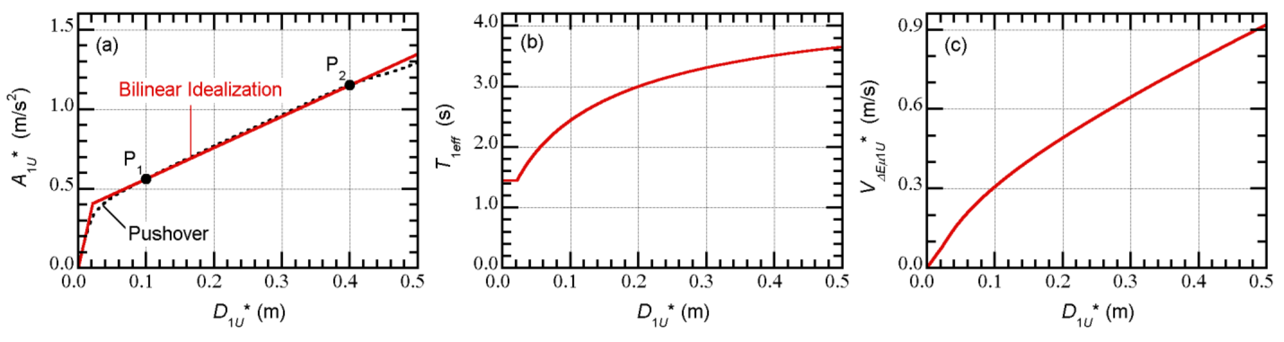
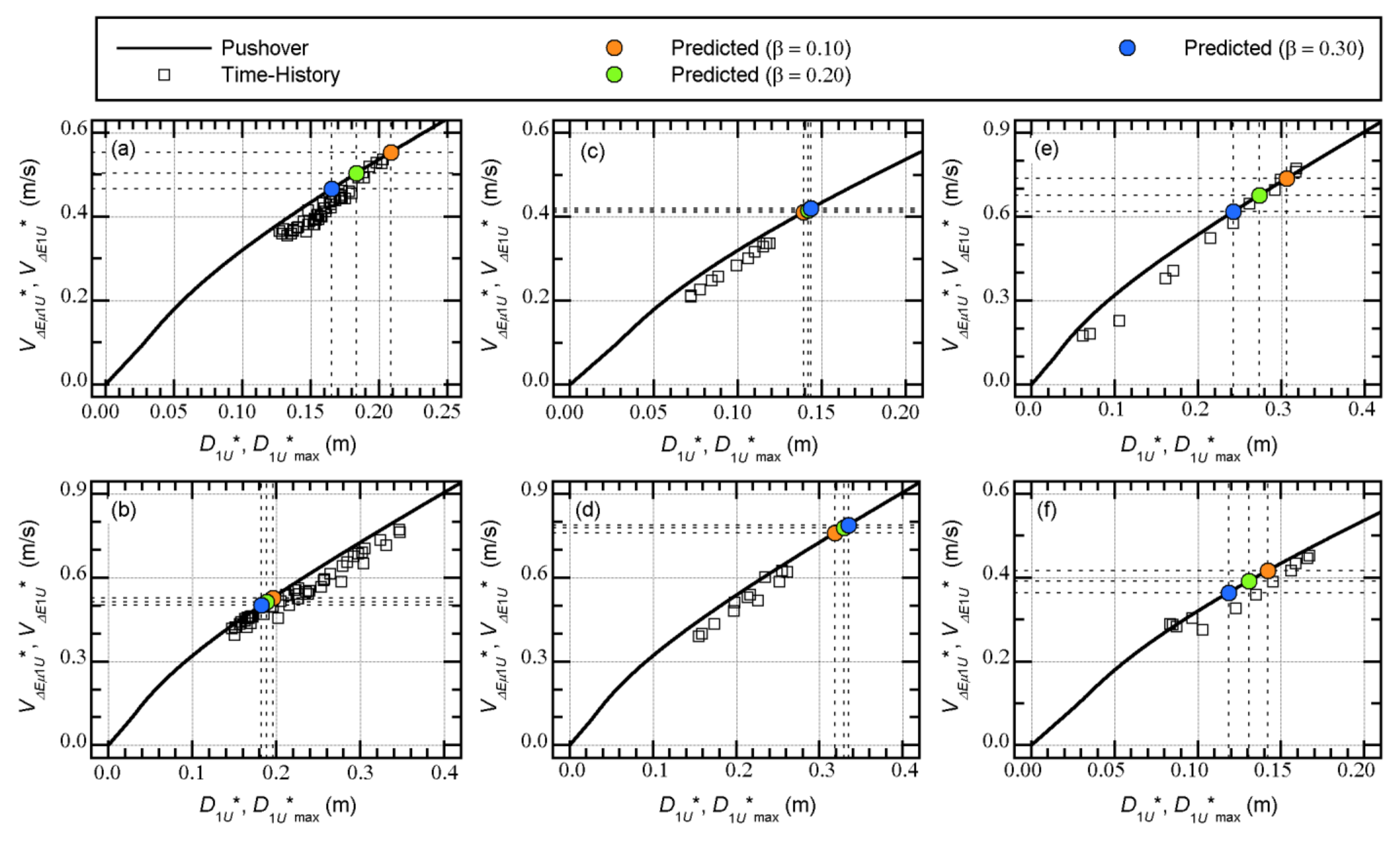
- The relationship between the equivalent velocity of the maximum momentary input energy of the first modal response () and the peak equivalent displacement of the first modal response () can be properly evaluated from the pushover analysis results. The plots obtained from the nonlinear time-history analysis results fit the evaluated curve from the pushover analysis results well.
- The upper bound of the peak equivalent displacements of the first two modal responses can be predicted using the bidirectional spectrum [52]. Comparisons between the predicted peak equivalent displacements and those calculated from the nonlinear time-history analysis results showed that the predicted peak approximated the upper bound of the nonlinear time-history analysis results. The upper bound of can be approximated by the bidirectional spectrum.
Author Contributions
Funding
Institutional Review Board Statement
Informed Consent Statement
Data Availability Statement
Acknowledgments
Conflicts of Interest
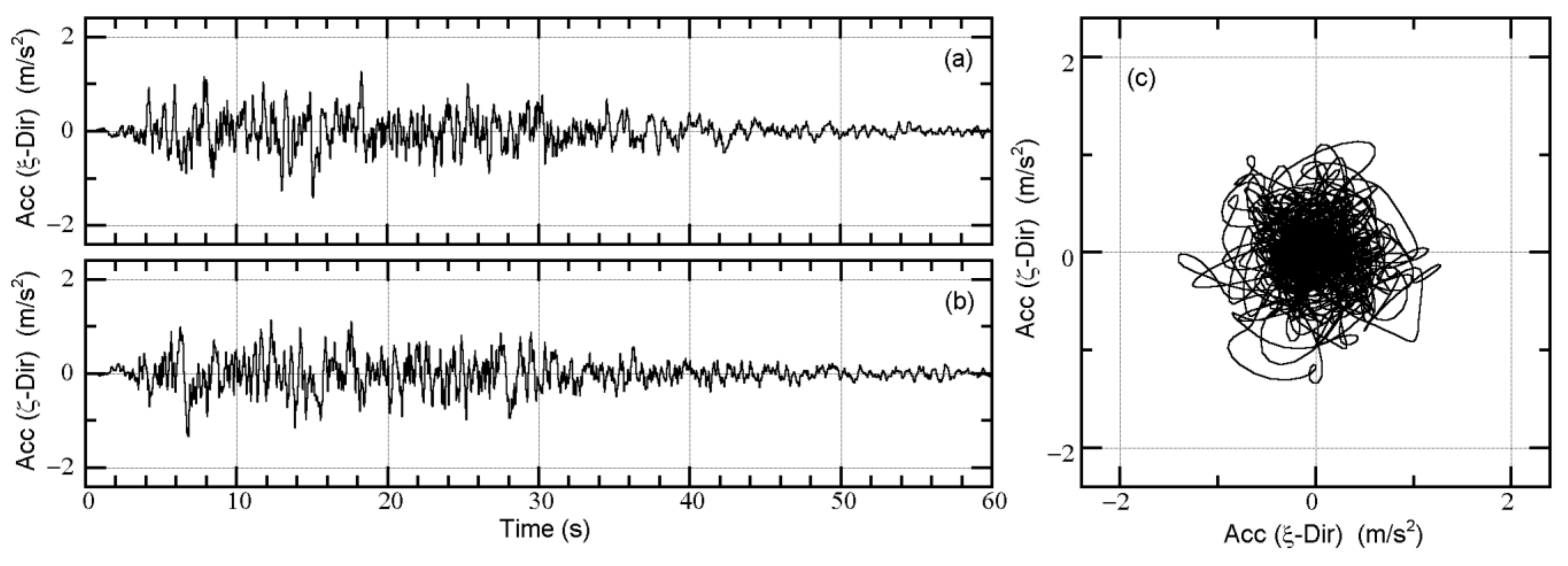
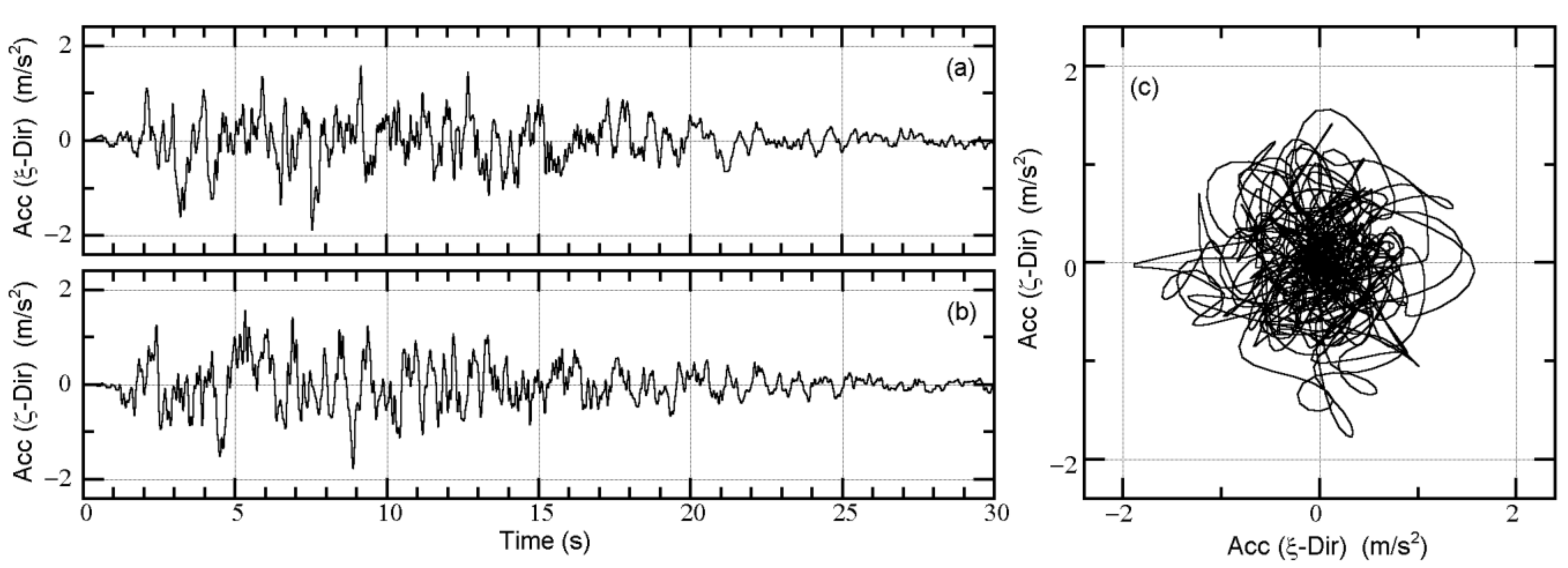
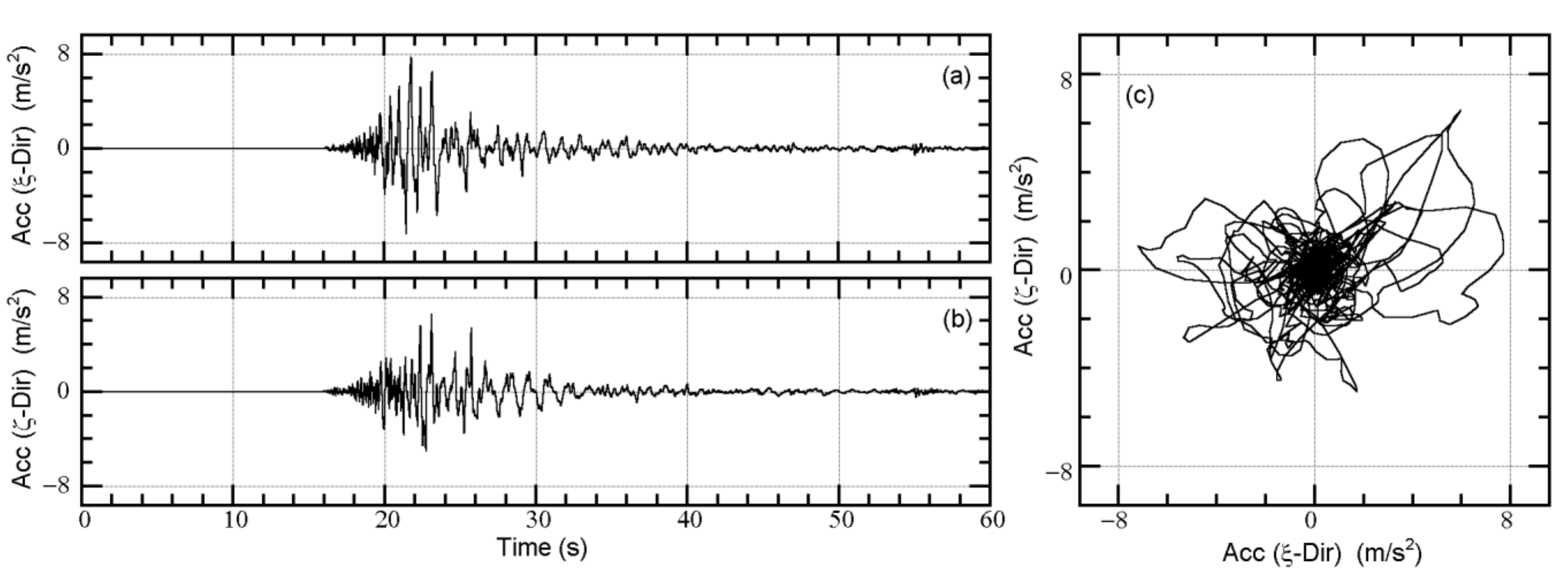
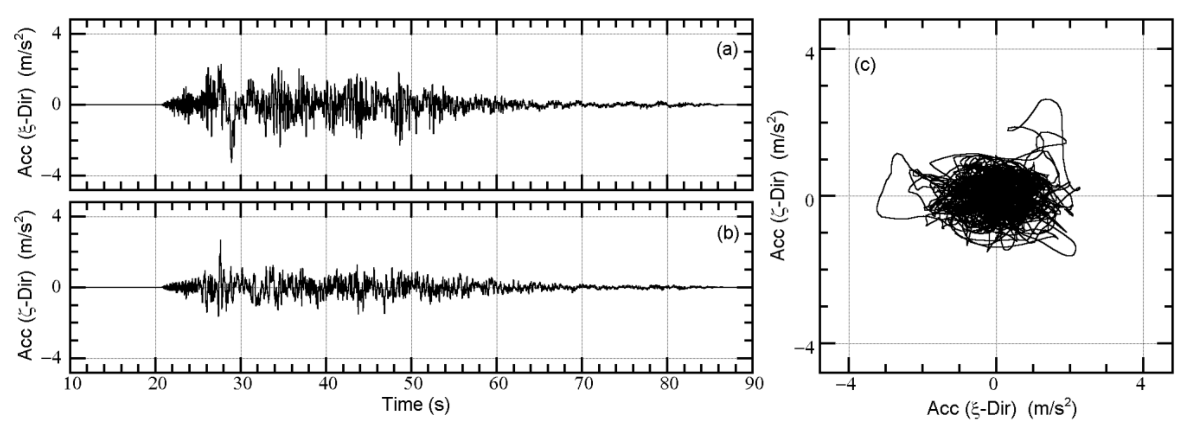
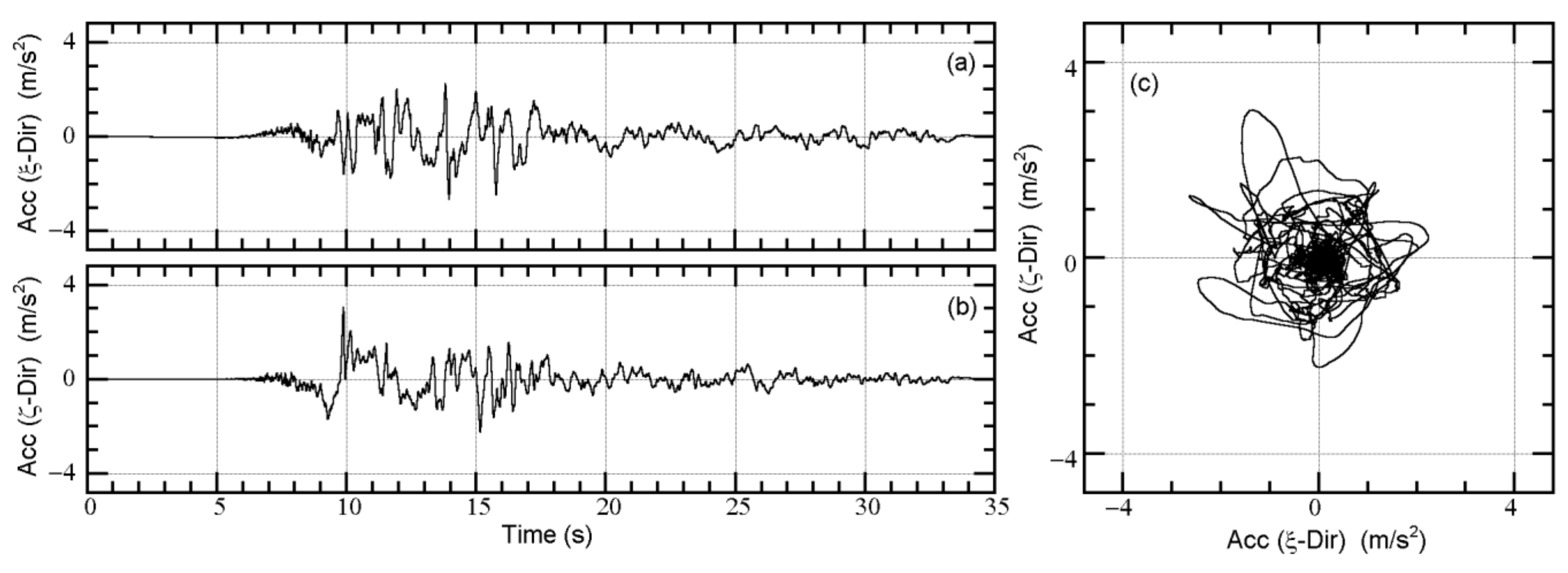
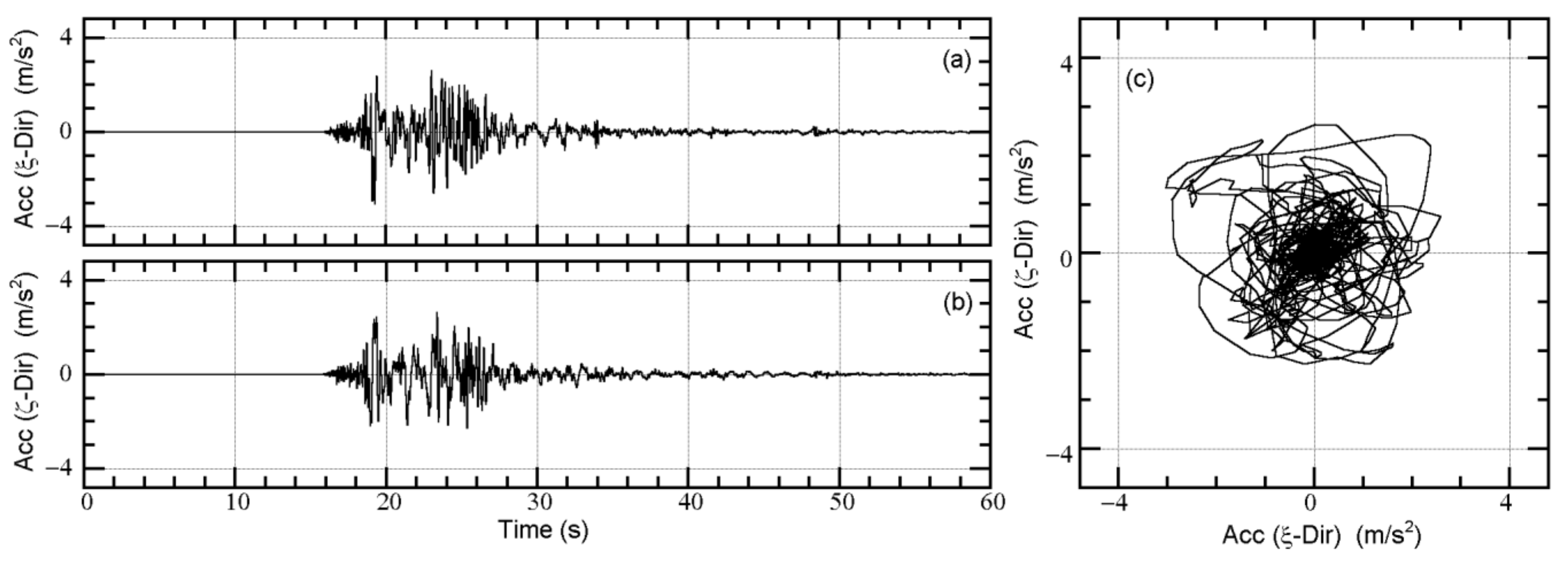
Appendix A. Time-Histories of the Recorded Ground Motions Used in This Study

| ID | Event Date | Magnitude | Distance | Station Name | Direction of Components | |
|---|---|---|---|---|---|---|
| ξ-Dir | ζ-Dir | |||||
| UTO0414 | 14 April 2016 | = 6.5 | 15 km | K-Net UTO (KMM008) | EW | NS |
| UTO0416 | 16 April 2016 | = 7.3 | 12 km | K-Net UTO (KMM008) | EW | NS |
| TCU | 20 September 1999 | = 7.6 | 0.89 km * | TCU075 | Major ** | Minor ** |
| YPT | 17 August 1999 | = 7.5 | 4.83 km * | Yarimca | Major ** | Minor ** |


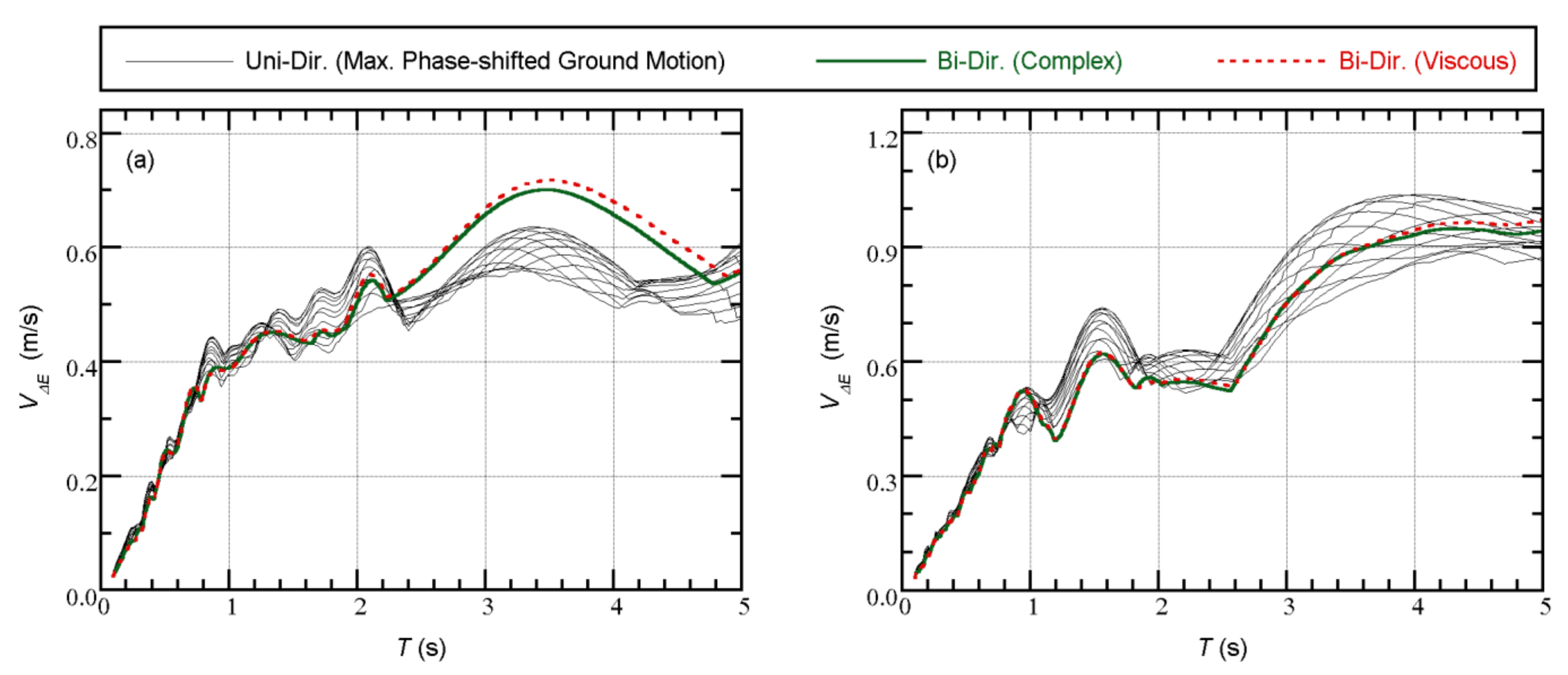
Appendix B. Comparisons of the Unidirectional and Bidirectional VΔE Spectra
References
- Charleson, A.; Guisasola, A. Seismic Isolation for Architects; Routledge: London, UK; New York, NY, USA, 2017. [Google Scholar]
- Architectural Institute of JAPAN (AIJ). Design Recommendations for Seismically Isolated Buildings; Architectural Institute of Japan: Tokyo, Japan, 2016. [Google Scholar]
- ASCE. Seismic Evaluation and Retrofit of Existing Buildings; ASCE Standard, ASCE/SEI41-17; American Society of Civil Engineering: Reston, VA, USA, 2017. [Google Scholar]
- Seki, M.; Miyazaki, M.; Tsuneki, Y.; Kataoka, K. A Masonry school building retrofitted by base isolation technology. In Proceedings of the 12th World Conference on Earthquake Engineering, Auckland, New Zealand, 30 January–4 February 2000. [Google Scholar]
- Kashima, T.; Koyama, S.; Iiba, M.; Okawa, I. Dynamic behaviour of a museum building retrofitted using base isolation system. In Proceedings of the 14th World Conference on Earthquake Engineering, Beijing, China, 12–17 October 2008. [Google Scholar]
- Clemente, P.; De Stefano, A. Application of seismic isolation in the retrofit of historical buildings. Earthquake Resistant Engineering Structures VIII; WIT Press: Southampton, UK, 2011; Volume 120, pp. 41–52. [Google Scholar]
- Gilani, A.S.; Miyamoto, H.K. Base isolation retrofit challenges in a historical monumental building in Romania. In Proceedings of the 15th World Conference on Earthquake Engineering, Lisbon, Portugal, 24–28 September 2012. [Google Scholar]
- Nakamura, H.; Ninomiya, T.; Sakaguchi, T.; Nakano, Y.; Konagai, K.; Hisada, Y.; Seki, M.; Ota, T.; Yamazaki, Y.; Mochizuki, S.; et al. Seismic isolation retrofit of Susano City Hall situated above lava tubes. In Proceedings of the 15th World Conference on Earthquake Engineering, Lisbon, Portugal, 24–28 September 2012. [Google Scholar]
- Sorace, S.; Terenzi, G. A viable base isolation strategy for the advanced seismic retrofit of an r/c building. Contemp. Eng. Sci. 2014, 7, 817–834. [Google Scholar] [CrossRef]
- Ferraioli, M.; Mandara, A. Base isolation for seismic retrofitting of a multiple building structure: Evaluation of equivalent linearization method. Math. Probl. Eng. 2016, 2016, 8934196. [Google Scholar] [CrossRef]
- Terenzi, G.; Fuso, E.; Sorace, S.; Costoli, I. Enhanced seismic retrofit of a reinforced concrete building of architectural interest. Buildings 2020, 10, 211. [Google Scholar] [CrossRef]
- Vailati, M.; Monti, G.; Bianco, V. Integrated solution-base isolation and repositioning-for the seismic rehabilitation of a preserved strategic building. Buildings 2021, 11, 164. [Google Scholar] [CrossRef]
- Usta, P. Investigation of a base-isolator system’s effects on the seismic behavior of a historical structure. Buildings 2021, 11, 217. [Google Scholar] [CrossRef]
- Nishizawa, T.; Suekuni, R. Outline of structural design for Kyoto City Hall. In Proceedings of the 17th World Conference on Earthquake Engineering, Sendai, Japan, 20 September–2 November 2021. [Google Scholar]
- Hashimoto, T.; Fujita, K.; Tsuji, M.; Takewaki, I. Innovative base-isolated building with large mass-ratio TMD at basement for greater earthquake resilience. Future Cities Environ. 2015, 1, 9. [Google Scholar] [CrossRef]
- Ikenaga, M.; Ikago, K.; Inoue, N. Development of a displacement-dependent damper for base isolated structures. In Proceedings of the Tenth International Conference on Computational Structures Technology, Valencia, Spain, 14–17 September 2010. [Google Scholar]
- Ikenaga, M.; Ikago, K.; Inoue, N. Seismic displacement control design of base isolated structures by magneto-rheological dampers based on a pseudo-complex-damping rule. In Proceedings of the Thirteenth International Conference on Computational Structures Technology, Crete, Greece, 6–9 September 2011. [Google Scholar]
- Nakaminami, S.; Ikago, K.; Inoue, N.; Kida, H. Response characteristics of a base-isolated structure incorporated with a force-restricted viscous mass damper. In Proceedings of the 15th World Conference on Earthquake Engineering, Lisbon, Portugal, 24–28 September 2012. [Google Scholar]
- Inoue, N.; Ikago, K. Displacement control design concept for long-period structures. In Proceedings of the 16th World Conference on Earthquake Engineering, Santiago, Chile, 9–13 January 2017. [Google Scholar]
- Anajafi, H.; Medina, R.A. Comparison of the seismic performance of a partial mass isolation technique with conventional TMD and base-isolation systems under broad-band and narrow-band excitations. Eng. Struct. 2018, 158, 110–123. [Google Scholar] [CrossRef]
- Luo, H.; Ikago, K.; Chong, C.; Keivan, A.; Phillips, B.M. Performance of low-frequency structures incorporated with rate-independent linear damping. Eng. Struct. 2019, 181, 324–335. [Google Scholar] [CrossRef]
- Tariq, M.A.; Usman, M.; Farooq, S.H.; Ullah, I.; Hanif, A. Investigation of the structural response of the MRE-based MDOF isolated structure under historic near- and far-fault earthquake loadings. Appl. Sci. 2021, 11, 2876. [Google Scholar] [CrossRef]
- Nagarajaiah, S.; Reinhorn, A.M.; Constantinou, M.C. Torsion in base-isolated structures with elastomeric isolation systems. J. Struct. Eng. ASCE 1992, 119, 2932–2951. [Google Scholar] [CrossRef]
- Tena-Colunga, A.; Gόmez-Soberόn, L. Torsional response of base-isolated structures due to asymmetries in the superstructure. Eng. Struct. 2002, 24, 1587–1599. [Google Scholar] [CrossRef]
- Tena-Colunga, A.; Zambrana-Rojas, C. Dynamic torsional amplifications of base-isolated structures with an eccentric isolation system. Eng. Struct. 2006, 28, 72–83. [Google Scholar] [CrossRef]
- Tena-Colunga, A.; Escamilla-Cruz, J.L. Torsional amplifications in asymmetric base-isolated structures. Eng. Struct. 2008, 29, 237–247. [Google Scholar] [CrossRef]
- Seguín, C.E.; De La Llera, J.C.; Almazán, J.L. Base–structure interaction of linearly isolated structures with lateral–torsional coupling. Eng. Struct. 2008, 30, 110–125. [Google Scholar] [CrossRef]
- Di Sarno, L.; Chioccarelli, E.; Cosenza, E. Seismic response analysis of an irregular base isolated building. Bull. Earthq. Eng. 2011, 9, 1673–1702. [Google Scholar] [CrossRef]
- Mazza, F.; Mazza, M. Nonlinear seismic analysis of irregular r.c. framed buildings base-isolated with friction pendulum system under near-fault excitations. Soil Dyn. Earthq. Eng. 2016, 90, 299–312. [Google Scholar] [CrossRef]
- Cancellara, D.; De Angelis, F. Assessment and dynamic nonlinear analysis of different base isolation systems for a multi-storey RC building irregular in plan. Comput. Struct. 2017, 180, 74–88. [Google Scholar] [CrossRef]
- Mazza, F. Seismic demand of base-isolated irregular structures subjected to pulse-type earthquakes. Soil Dyn. Earthq. Eng. 2018, 108, 111–129. [Google Scholar] [CrossRef]
- Volcev, R.; Postolov, N.; Todorov, K.; Lazarov, L. Base isolation as an effective tool for plan irregularity reduction. In Seismic Behaviour and Design of Irregular and Complex Civil Structures III; Köber, D., De Stefano, M., Zembaty, Z., Eds.; Springer Nature Switzerland: Cham, Switzerland, 2020; pp. 377–389. [Google Scholar]
- Köber, D.; Semrau, P.; Weber, F. Design approach for an irregular hospital building in Bucharest. In Proceedings of the 9th European Workshop on the Seismic Behaviour of Irregular and Complex Structures, Online, 15–16 December 2020. [Google Scholar]
- Reyes, J.C. Seismic behaviour of torsionally-weak buildings with and without base isolators. In Proceedings of the 9th European Workshop on the Seismic Behaviour of Irregular and Complex Structures, Online, 15–16 December 2020. [Google Scholar]
- Koren, D.; Kilar, V. Seismic behaviour of asymmetric base isolated structures with various distributions of isolators. Eng. Struct. 2009, 31, 910–921. [Google Scholar]
- Koren, D.; Kilar, V. The applicability of the N2 method to the estimation of torsional effects in asymmetric base-isolated buildings. Earthq. Eng. Struct. Dyn. 2011, 40, 867–886. [Google Scholar] [CrossRef]
- Peruś, I.; Fajfar, P. On the inelastic torsional response of single-storey structures under bi-axial excitation. Earthq. Eng. Struct. Dyn. 2005, 34, 931–941. [Google Scholar] [CrossRef]
- Fajfar, P.; Marušić, D.; Peruś, I. Torsional effects in the pushover-based seismic analysis of buildings. J. Earthq. Eng. 2005, 9, 831–854. [Google Scholar] [CrossRef]
- Fujii, K. Nonlinear static procedure for multi-story asymmetric frame buildings considering bi-directional excitation. J. Earthq. Eng. 2011, 15, 245–273. [Google Scholar] [CrossRef]
- Fujii, K. Prediction of the largest peak nonlinear seismic response of asymmetric buildings under bi-directional excitation using pushover analyses. Bull. Earthq. Eng. 2014, 12, 909–938. [Google Scholar] [CrossRef]
- Fujii, K. Application of the pushover-based procedure to predict the largest peak response of asymmetric buildings with buckling-restrained braces. In Proceedings of the 5th ECCOMAS Thematic Conference on Computational Methods in Structural Dynamics and Earthquake Engineering (COMPDYN), Crete Island, Greece, 25–27 May 2015. [Google Scholar]
- Fujii, K. Assessment of pushover-based method to a building with bidirectional setback. Earthq. Struct. 2016, 11, 421–443. [Google Scholar] [CrossRef]
- Fujii, K. Prediction of the peak seismic response of asymmetric buildings under bidirectional horizontal ground motion using equivalent SDOF model. Jpn. Archit. Rev. 2018, 1, 29–43. [Google Scholar] [CrossRef] [Green Version]
- Fujii, K. Pushover-based seismic capacity evaluation of Uto City Hall damaged by the 2016 Kumamoto Earthquake. Buildings 2019, 9, 140. [Google Scholar] [CrossRef] [Green Version]
- Building Center of Japan (BCJ). The Building Standard Law of Japan on CD-ROM; The Building Center of Japan: Tokyo, Japan, 2016. [Google Scholar]
- Güneş, N.; Ulucan, Z.Ç. Nonlinear dynamic response of a tall building to near-fault pulse-like ground motions. Bull. Earthq. Eng. 2019, 17, 2989–3013. [Google Scholar] [CrossRef]
- Akiyama, H. Earthquake–Resistant Limit–State Design for Buildings; University of Tokyo Press: Tokyo, Japan, 1985. [Google Scholar]
- Nakamura, T.; Hori, N.; Inoue, N. Evaluation of damaging properties of ground motions and estimation of maximum displacement based on momentary input energy. J. Struct. Constr. Eng. AIJ 1998, 513, 65–72. (In Japanese) [Google Scholar] [CrossRef]
- Inoue, N.; Wenliuhan, H.; Kanno, H.; Hori, N.; Ogawa, J. Shaking Table Tests of Reinforced Concrete Columns Subjected to Simulated Input Motions with Different Time Durations. In Proceedings of the 12th World Conference on Earthquake Engineering, Auckland, New Zealand, 30 January–4 February 2000. [Google Scholar]
- Hori, N.; Inoue, N. Damaging properties of ground motion and prediction of maximum response of structures based on momentary energy input. Earthq. Eng. Struct. Dyn. 2002, 31, 1657–1679. [Google Scholar] [CrossRef]
- Fujii, K.; Kanno, H.; Nishida, T. Formulation of the time-varying function of momentary energy input to a SDOF system by Fourier series. J. Jpn. Assoc. Earthq. Eng. 2019, 19, 247–266. (In Japanese) [Google Scholar] [CrossRef]
- Fujii, K.; Murakami, Y. Bidirectional momentary energy input to a one-mass two-DOF system. In Proceedings of the 17th World Conference on Earthquake Engineering, Sendai, Japan, 20 September–2 November 2021. [Google Scholar]
- Fujii, K. Bidirectional seismic energy input to an isotropic nonlinear one-mass two-degree-of-freedom system. Buildings 2021, 11, 143. [Google Scholar] [CrossRef]
- Strong-Motion Seismograph Networks (K-NET, KiK-net). Available online: https://www.kyoshin.bosai.go.jp/ (accessed on 14 October 2021).
- Bridgestone Corporation. Seismic Isolation Product Line-Up. Version 2017. Volume 1. Available online: https://www.bridgestone.com/products/diversified/antiseismic_rubber/pdf/catalog_201710.pdf (accessed on 7 September 2021).
- Bridgestone Corporation. Kenchiku-Menshin-yo Sekisou-Gomu-Seihin Shiyou-Ichiran (Seismic Isolation Product Line-Up). Version 2021. Volume 1. Available online: https://www.bridgestone.co.jp/products/dp/antiseismic_rubber/product/pdf/product_catalog_202106.pdf (accessed on 7 September 2021).
- Nippon Steel Engineering Co. Ltd. Men-Shin NSU Damper Line-Up. Available online: https://www.eng.nipponsteel.com/steelstructures/product/base_isolation/damper_u/lineup_du/ (accessed on 3 August 2019). (In Japanese).
- Fujii, K. Prediction of the Maximum Seismic Member Force in a Superstructure of a Base-Isolated Frame Building by Using Pushover Analysis. Buildings 2019, 9, 201. [Google Scholar] [CrossRef] [Green Version]
- Wada, A.; Hirose, K. Elasto-plastic dynamic behaviors of the building frames subjected to bi-directional earthquake motions. J. Struct. Constr. Eng. AIJ 1989, 399, 37–47. (In Japanese) [Google Scholar]
- Almansa, F.L.; Weng, D.; Li, T.; Alfarah, B. Suitability of seismic isolation for buildings founded on soft soil. Case study of a RC building in Shanghai. Buildings 2020, 10, 241. [Google Scholar] [CrossRef]
- Ordaz, M.; Huerta, B.; Reinoso, E. Exact Computation of Input-Energy Spectra from Fourier Amplitude Spectra. Earthq. Eng. Struct. Dyn. 2003, 32, 597–605. [Google Scholar] [CrossRef]
- Kuramoto, H. Earthquake response characteristics of equivalent SDOF system reduced from multi-story buildings and prediction of higher mode responses. J. Struct. Constr. Eng. AIJ 2004, 580, 61–68. (In Japanese) [Google Scholar] [CrossRef] [Green Version]
- Arias, A. A measure of seismic intensity. In Seismic Design for Nuclear Power Plant; MIT Press: Cambridge, MA, USA, 1970; pp. 438–483. [Google Scholar]
- Penzien, J.; Watabe, M. Characteristics of 3-dimensional earthquake ground motions. Earthq. Eng. Struct. Dyn. 1975, 3, 365–373. [Google Scholar] [CrossRef]
- Boore, D.M.; Watson-Lamprey, J.; Abrahamson, N.A. Orientation-Independent Measures of Ground Motion. Bull. Seismol. Soc. Am. 2007, 96, 1502–1511. [Google Scholar] [CrossRef]


| Floor Level j | Floor Mass mj (t) | Moment of Inertia Ij (×103 tm2) | Radius of Gyration of Floor Mass rj (m) |
|---|---|---|---|
| 5 | 677.8 | 78.37 | 10.75 |
| 4 | 548.5 | 62.85 | 10.70 |
| 3 | 543.0 | 62.50 | 10.73 |
| 2 | 581.0 | 67.12 | 10.75 |
| 1 | 1208.1 | 199.0 | 12.83 |
| 0 | 1853.7 | 274.9 | 12.18 |
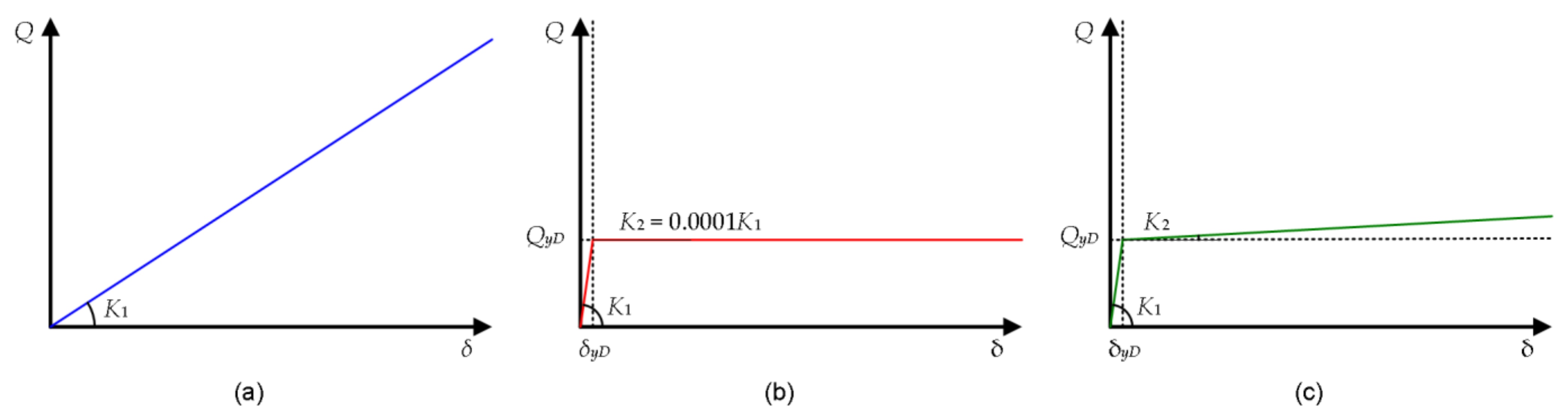
| Type | Outer Diameter (mm) | Total Rubber Thickness (mm) | Shear Modulus (MPa) | Horizontal Stiffness K1 (MN/m) | Vertical Stiffness KV (MN/m) |
|---|---|---|---|---|---|
| NRB (ϕ = 900 mm, G5) | 900 | 180 | 0.441 | 1.56 | 3730 |
| NRB (ϕ = 900 mm, G4) | 900 | 180 | 0.392 | 1.38 | 3420 |
| Type | Outer Diameter (mm) | Shear Modulus (MPa) | Friction Coefficient μ | Initial Horizontal Stiffness K1 (MN/m) | Vertical Stiffness KV (MN/m) |
|---|---|---|---|---|---|
| ESB (ϕ = 300 mm) | 300 | 0.392 | 0.010 | 0.884 | 1380 |
| ESB (ϕ = 400 mm) | 400 | 0.392 | 0.010 | 1.48 | 2270 |
| ESB (ϕ = 500 mm) | 500 | 0.392 | 0.010 | 2.40 | 3710 |
| Initial Stiffness K1 (MN/m) | Yield Strength Qyd (kN) | Post Yield Stiffness K2 (MN/m) |
|---|---|---|
| 7.60 | 184 | 0.128 |
| Earthquake of the Original Record | Ground Motion ID | Scale Factor | |
|---|---|---|---|
| Model-Tf34 | Model-Tf44 | ||
| Kumamoto, 14 April 2016 | UTO0414 | 1.000 | 1.000 |
| Kumamoto, 16 April 2016 | UTO0416 | 1.000 | 1.000 |
| Chichi, 1999 | TCU | 0.5540 | 0.5718 |
| Kocaeli, 1999 | YPT | 0.4293 | 0.5057 |
| Ground Motion Set | First Mode VΔE(T1eff) (m/s) | Second Mode VΔE(T2eff) (m/s) | Third Mode VΔE(T3e) (m/s) | Ratio (2nd/1st) | Ratio (3rd/1st) |
|---|---|---|---|---|---|
| UTO0414 | 0.4108 | 0.4232 | 0.7151 | 1.030 | 1.741 |
| TCU | 0.7575 | 0.7319 | 0.2519 | 0.9662 | 0.3325 |
Publisher’s Note: MDPI stays neutral with regard to jurisdictional claims in published maps and institutional affiliations. |
© 2021 by the authors. Licensee MDPI, Basel, Switzerland. This article is an open access article distributed under the terms and conditions of the Creative Commons Attribution (CC BY) license (https://creativecommons.org/licenses/by/4.0/).
Share and Cite
Fujii, K.; Masuda, T. Application of Mode-Adaptive Bidirectional Pushover Analysis to an Irregular Reinforced Concrete Building Retrofitted via Base Isolation. Appl. Sci. 2021, 11, 9829. https://doi.org/10.3390/app11219829
Fujii K, Masuda T. Application of Mode-Adaptive Bidirectional Pushover Analysis to an Irregular Reinforced Concrete Building Retrofitted via Base Isolation. Applied Sciences. 2021; 11(21):9829. https://doi.org/10.3390/app11219829
Chicago/Turabian StyleFujii, Kenji, and Takumi Masuda. 2021. "Application of Mode-Adaptive Bidirectional Pushover Analysis to an Irregular Reinforced Concrete Building Retrofitted via Base Isolation" Applied Sciences 11, no. 21: 9829. https://doi.org/10.3390/app11219829
APA StyleFujii, K., & Masuda, T. (2021). Application of Mode-Adaptive Bidirectional Pushover Analysis to an Irregular Reinforced Concrete Building Retrofitted via Base Isolation. Applied Sciences, 11(21), 9829. https://doi.org/10.3390/app11219829