Distributed Control for Coordinated Tracking of Fixed-Wing Unmanned Aerial Vehicles under Model Uncertainty and Disturbances

Abstract

In this paper, we consider a control problem where a group of fixed-wing unmanned aerial vehicles (UAVs) with uncertain dynamics tracks the target vehicle cooperatively in the case of external disturbance. Based on the Gaussian process regression, a data-driven model is established, whose uniform error is bounded with probability. Then a learning-based consensus protocol for multi-UAVs is designed. The stability of the system is proven via Lyapunov function, and the tracking error is guaranteed to be bounded with a high probability. Finally, the effectiveness of the proposed method is shown in the numerical simulation.

1. Introduction

In recent years, cooperative tracking control of multi-UAVs has been developing rapidly for its wide application [1,2], such as pursuing recovery device in air-recovery [3], following aircraft in a cooperative operation [4] and tracking virtual leader in formation flight [5]. However, there exist many challenges in the research [2]. First, the nonlinear dynamics, in particular the unmodeled dynamics, of UAV make the design of control law more difficult. Second, the disturbance in the environment, such as wind, is to be considered in the coordinated control for the safety of the formation flight.

For the study of the model of fixed-wing UAV, 6 DOF model [6] is constructed in the early modeling of UAV, where aerodynamic parameters are used to refine the model characteristics. However, it is difficult to be applied in practice due to the coupling characteristics of the model and it is usually used in the maneuver flight with high speed, which relies on the attitude control [7]. To better analyze the movement of UAV in three-dimensional, most researchers adopt 3 DOF model [8,9] in their study. Furthermore, if the height remains unchanged, the 3 DOF model can be expressed as a unicycle model [10,11], which is a kinematic model without considering the dynamic characteristics of the UAV. To better analyze the tracking performance of the UAVs in the plane, a 2 DOF model is discussed in this paper based on the assumption that the height of the UAV is constant, which not only preserves the dynamics of the UAV but also simplifies the description of the problem.

Although most of the models we use are the nominal model, which is a standard model without uncertainties, there is still an uncertain part caused by parameter uncertainties and high-order dynamic terms, which is often difficult to be modeled by functions. Thus, data-driven model is widely used in the model-based control techniques with the development of computer technology. Gaussian process (GP) model is a Bayesian nonparametric regression model, which is widely used in the machine learning [12,13]. Compared with the neural networks (NNs) [9], GP does not only provide a prediction but also a prediction variance, an effective measure of the uncertainty of the learned model [14]. When model-based methods are used in control, model errors are of great importance to be taken into account [15]. GP provides uniform error bound [16,17], while there is no guaranteed bound of the estimation error in NNs [18]. To apply model-based control methods to data-driven models, we use GP regression to model the unknown dynamics of the UAV for its uniform error bound.

The main contribution of this paper is the design of a cooperative tracking control law for fixed-wing unmanned aerial vehicles based on GP, considering model uncertainty and disturbances. We model the unknown dynamics of fixed-wing UAV based on GP, take the disturbance into account, prove the stability of the system with the help of Lyapunov function and guarantee that the tracking errors are in a certain bound with a high probability.

The remainder of the paper is as follows: Section 2 reviews the works related to our research. In Section 3, some mathematical symbols are explained, and the basic knowledge of graph theory and Gaussian process regression is introduced. The mathematical description of control problem is established in Section 4 followed by the main results of our work in Section 5, where the learning-based control law for coordinated tracking is proposed and stability with probability for the system is proven. Section 6 shows the results of numerical simulation and demonstrates the effectiveness of the proposed method. Conclusion is drawn in Section 7.

2. Related Work

There are many applications based on Gaussian process, such as constructing maps [19], filtering [20], action recognition [21], classification of hyperspectral images [22,23] and modeling. In particular, modeling is one of the most important applications. Jongseok Lee et al. [24] proposed an identification framework for fixed-wing platforms, which includes flight test, training parameter, correcting identification and updating model. Khansari-Zadeh et al. [25] presented a method to learn discrete robot motions and demonstrates its validity through a set of robot experiments. With the wide applications of GP model, some researchers started to apply control methods to GP model. Prasad Hemakumara et al. [26] modeled the dynamic of UAV and controlled it in real flight. Sooho Park et al. [27] proposed a learning algorithm to learn the unknown system model and tested it on the control of the mecanum-wheeled robot. It is a pity that the above research lacks analysis of stability of the control system.

When it comes to the stability of control system based on GP model, we have to thank Niranjan Srinivas et al. [16] for their excellent work. They obtained explicit sublinear regret bounds for many commonly used covariance functions, which is cited by many researchers. Based on their theory, Jonas Umlauft et al. [28] put forward an uncertainty-based control Lyapunov function framework to stabilize control-affine systems with high probability, while Michael Maiworm et al. [14,29] designed a model predictive control law for nonlinear discrete time systems and established input-to-state stability. Armin Lederer et al. derived a novel uniform error bound under weaker assumptions.

All the research above applies to individuals. There exists a few data-driven control approaches for unknown nonlinear multi-agent systems (MAS) [18]. Zewen Yang et al. [18] designed a learning-based leader-follower consensus protocol for unknown nonlinear MAS based on GP. However, the model proposed by Zewen Yang et al. is relatively simple and does not apply to the design of control law of fixed-wing UAV, at the same time, the disturbance caused by changing wind and mutual airflow between UAVs is not considered, which is of great importance in the control of multi-UAVs. Although Wang Ping et al. [30]. and Michael Defoort et al [31]. had taken disturbance into account, they did not consider the uncertain dynamics of agents. Inspired by them, we design a cooperative tracking control law for fixed-wing unmanned aerial vehicles based on GP, considering model uncertainty and disturbance, and prove the stability of the proposed method.

3. Preliminaries

3.1. Notation

In this paper, vectors and matrices are represented by bold letters, while scalars are represented by normal letters. For a vector $\mathit{x}\in {\mathbb{R}}^n$, $\parallel \mathit{x}\parallel$ is usual Euclidean norm of $\mathit{x}$, i.e., $\parallel \mathit{x}\parallel ={\left({\sum }_{i=1}^n{|x_i|}^2\right)}^{\frac{1}{2}}$. Accordingly, the matrix norm is induced by Euclidean norm i.e., for a matrix $\mathit{A}\in {\mathbb{R}}^{m\times n}$, $∥\mathit{A}∥=\sqrt{max\left\{{\lambda }_i\left({\mathit{A}}^H\mathit{A}\right)\right\}}$, where ${\mathit{A}}^H$ is the conjugate transpose of $\mathit{A}$ and ${\lambda }_i\left(\mathit{A}\right)$ is the i-th eigenvalue of $\mathit{A}$. For a square matrix $\mathit{B}\in {\mathbb{R}}^{n\times n}$, the expression $\mathit{B}\prec \mathbf{0}$ means $\mathit{B}$ is a negative definite matrix, while $\mathit{B}\succ \mathbf{0}$ means $\mathit{B}$ is a positive definite matrix. The symbol ⊗ denotes the Kronecker product, e.g., for matrix $\mathit{C}\in {\mathbb{R}}^{m\times n},\mathit{D}\in {\mathbb{R}}^{p\times q}$,

$$\mathit{C}\otimes \mathit{D}=\left[\begin{array}{ccc}{c}_{11}\mathit{D}& \cdots & c_{1n}\mathit{D}\\ ⋮& \ddots & ⋮\\ c_{m1}\mathit{D}& \cdots & c_{mn}\mathit{D}\end{array}\right]\in {\mathbb{R}}^{mp\times nq},$$

where $c_{ij}$ is the $ij$-th element of $\mathit{C}$.

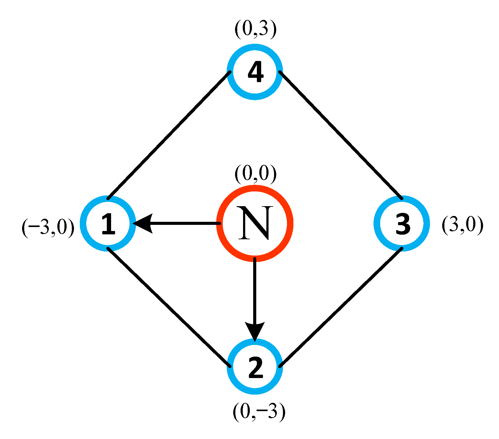
3.2. Graph Theory

We use an undirected graph $\mathcal{G}=(\mathcal{V},\mathcal{E})$ to describe the interactions among a group of n fixed-wing UAVs, where $\mathcal{V}=\left\{1,\cdots ,n\right\}$ is a node set, $\mathcal{E}\subseteq \mathcal{V}\times \mathcal{V}$ is a set of ordered pairs of nodes, called edges. The adjacency matrix $\mathit{A}={\left[a_{ij}\right]}_{n\times n}$ is defined as $a_{ii}=0$ and $a_{ij}=a_{ji}=1$ if there is an edge between node i and node j. Diagonal matrix $\mathit{D}=diag\left\{d_{11},d_{22},\cdots ,d_{nn}\right\}$ is the degree matrix of $\mathcal{G}$, where the element of $d_{ii}={\sum }_{j=1}^n{a}_{ij}$. The Laplacian matrix of the graph $\mathcal{G}$ is defined as $\mathit{L}=\mathit{D}-\mathit{A}$. Without loss of generality, the UAVs are denoted by nodes $1,2,\cdots ,n$, and the target vehicle is denoted by node 0. We use another diagonal matrix $\mathit{B}=diag\left\{b_{11},b_{22},\cdots ,b_{nn}\right\}$ to describe the connection between the i-th UAV and the target vehicle, where $b_{ii}>0$ if the state of the target is available to the i-th UAV and $b_{ii}=0$ otherwise.

The following assumption is made on digraph $\mathcal{G}$.

Assumption 1.

The undirected graph $\mathcal{G}$ is connected and there exists at least one UAV that can obtains the state of the target.

Based on the Assumption 1, there are two important lemmas as follows

Lemma 1.

Let $\mathit{L}=\left(l_{ij}\right)\in {\mathbb{R}}^{n\times n}$ be a Laplacian matrix of a connected undirected graph. Then the matrix

$$\tilde{\mathit{L}}=\mathit{L}+\mathit{B}=\left[\begin{array}{ccc}{l}_{11}+b_{11}& \cdots & l_{1n}\\ ⋮& \ddots & ⋮\\ l_{n1}& \cdots & l_{nn}+b_{nn}\end{array}\right],$$

(1)

is positive definite, if there exists an i such that$b_{ii}>0$.

Proof of Lemma 1.

For $\forall \mathit{z}\in \mathbb{R}{}^n\setminus \left\{\mathbf{0}\right\}$, one can obtain that ${\mathit{z}}^T\tilde{\mathit{L}}\mathit{z}={\mathit{z}}^T\mathit{L}\mathit{z}+{\mathit{z}}^T\mathit{B}\mathit{z}\ge 0$, since $\mathit{L}$ and $\mathit{B}$ are both positive semi-definite. When ${\mathit{z}}^T\mathit{L}\mathit{z}=0$, one can obtain that $\mathit{z}\in span\left\{\mathbf{1}\right\}\backslash \left\{\mathbf{0}\right\}$, and ${\mathit{z}}^T\mathit{B}\mathit{z}>0$. Thus, we always have ${\mathit{z}}^T\tilde{\mathit{L}}\mathit{z}>0$ for $\mathit{z}\ne 0$, which implies the conclusion. □

Lemma 2.

Let $\tilde{\mathit{L}}\in {\mathbb{R}}^{n\times n}$ be a positive definite and symmetric matrix. Then the matrix

$$\mathit{M}=\left[\begin{array}{cc}\mathbf{0}& {\mathit{I}}_n\\ -{\beta }_1\tilde{\mathit{L}}& -{\beta }_2\tilde{\mathit{L}}\end{array}\right]\in {\mathbb{R}}^{2n\times 2n},$$

(2)

is negative definite, where${\beta }_1,{\beta }_2>0$.

Proof of Lemma 2.

To prove that $\mathit{M}\prec \mathbf{0}$, we can solve the equation $det(\lambda {\mathit{I}}_{2n}-\mathit{M})=0$, where $det(\lambda {\mathit{I}}_{2n}-\mathit{M})$ is the characteristic polynomial of matrix $\mathit{M}$. Please note that

$$\begin{array}{cc}det\left(\lambda {\mathit{I}}_{2n}-\mathit{M}\right)\hfill & =det\left(\left[\begin{array}{cc}\lambda {\mathit{I}}_n& -{\mathit{I}}_n\\ {\beta }_1\tilde{\mathit{L}}& \lambda {\mathit{I}}_n+{\beta }_2\tilde{\mathit{L}}\end{array}\right]\right)\hfill \\ \hfill & =det\left(\left[\begin{array}{cc}0& -{\mathit{I}}_n\\ {\lambda }^2{\mathit{I}}_n+\left({\beta }_1+{\beta }_2\lambda \right)\tilde{\mathit{L}}& \lambda {\mathit{I}}_n+{\beta }_2\tilde{\mathit{L}}\end{array}\right]\right)\hfill \\ \hfill & =det\left({\lambda }^2{\mathit{I}}_n+\left({\beta }_1+{\beta }_2\lambda \right)\tilde{\mathit{L}}\right)\hfill \end{array},$$

(3)

Additionally note that the eigenvalues of $\tilde{\mathit{L}}$ satisfy the following property

$$det\left(\lambda {\mathit{I}}_{2n}+\tilde{\mathit{L}}\right)=\prod _{i=1}^n\left(\lambda +{\rho }_i\right)$$

(4)

where ${\rho }_i$ is the i-th eigenvalues of $\tilde{\mathit{L}}$. Comparing Equation (3) and Equation (4), one can obtain that [32]

$$det\left({\lambda }^2{\mathit{I}}_n+\left({\beta }_1+{\beta }_2\lambda \right)\tilde{\mathit{L}}\right)=\prod _{i=1}^n\left({\lambda }^2+\left({\beta }_1+{\beta }_2\lambda \right){\rho }_i\right)$$

(5)

which implies that the roots of Equation (3) can be found by solving ${\lambda }^2+\left({\beta }_1+{\beta }_2\lambda \right){\rho }_i=0$. Thus, the eigenvalues of $\mathit{M}$ are given by

$${\lambda }_{i\pm }=\frac{-{\beta }_2{\rho }_i\pm \sqrt{{\beta }_2^2{\rho }_i^2-4{\beta }_1{\rho }_i}}{2}$$

(6)

Since $\tilde{\mathit{L}}\succ \mathbf{0}$, one can obtain that ${\rho }_i>0$, it is easy to prove that every eigenvalue of $\tilde{\mathit{L}}$ has negative real parts when ${\beta }_1,{\beta }_2>0$. Thus, $\mathit{M}\prec \mathbf{0}$. □

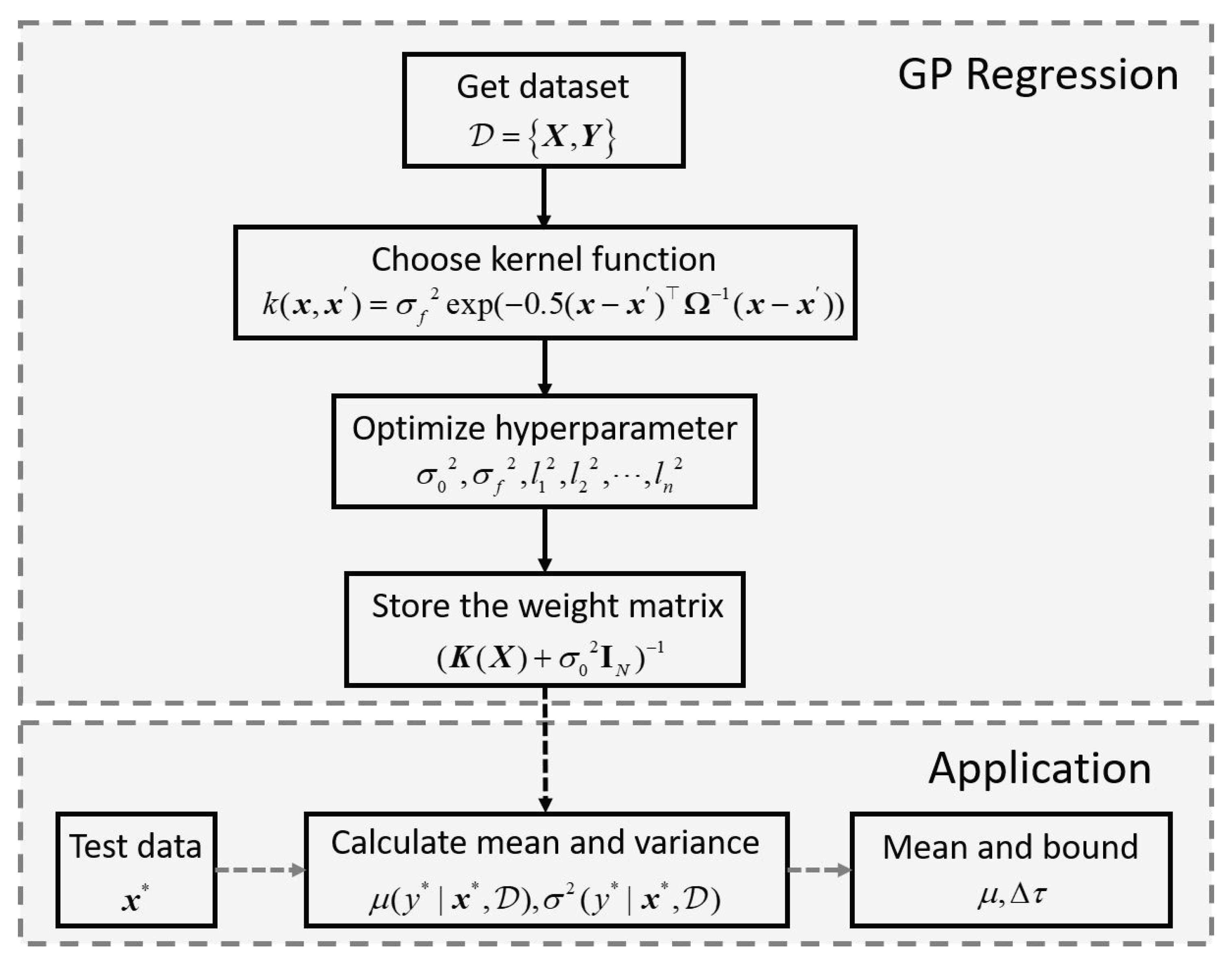
3.3. Gaussian Process Regression

For the learning of an unknown function $f(·)$, we need an oracle to predict the value of $f\left(\mathit{x}\right)$ for a given input $\mathit{x}\in \mathbb{X}$. In this paper, we use gaussian process as oracle which is a nonparametric model.

Definition 1

([33]). A gaussian process is a collection of random variables, any finite number of which have a joint Gaussian distribution.

Compared with other machine learning methods, GP does not only provide a prediction but also a prediction variance, an effective measure of the uncertainty of the learned model.

A GP is used to describe a distribution over functions, which can be written as

$$f\left(\mathit{x}\right)\sim \mathcal{G}\mathcal{P}\left(m\left(\mathit{x}\right),k\left(\mathit{x},{\mathit{x}}^{\prime }\right)\right),$$

(7)

where $m\left(\mathit{x}\right):\mathbb{X}\to \mathbb{R}$ is the prior mean function, which allows the inclusion of prior knowledge about the unknown function $f\left(\mathit{x}\right)$ and is often set to zero if there do not have any prior knowledge, and $k(\mathit{x},{\mathit{x}}^{\prime }):\mathbb{X}\times \mathbb{X}\to {\mathbb{R}}_{0,+}$ is the covariance function, which is associated with abstract concepts of function $f\left(\mathit{x}\right)$ such as smoothness. Since the choice of kernel function is beyond the research of this paper, we choose squared exponential kernel typically as kernel function

$$k(\mathit{x},{\mathit{x}}^{\prime })={{\sigma }_f}^{2}exp\left(-\frac{1}{2}{(\mathit{x}-{\mathit{x}}^{\prime })}^{\top }{\Omega }^{-1}(\mathit{x}-{\mathit{x}}^{\prime })\right),$$

(8)

where ${\sigma }_f\ge 0$, $\Omega =diag\{{l_1}^2,{l_2}^2,\cdots ,{l_n}^2\},l_i\ge 0$ are hyperparameters.

To explain the process of GP regression, we assume a training data set $\mathcal{D}=\left\{\mathit{X},\mathit{Y}\right\}$ consisting of training inputs $\mathit{X}=\left\{{\mathit{x}}^{\left(1\right)},{\mathit{x}}^{\left(2\right)},\cdots ,{\mathit{x}}^{\left(M\right)}\right\}$ and training outputs $\mathit{Y}=\left\{y^{\left(1\right)},y^{\left(2\right)},\cdots ,y^{\left(M\right)}\right\}$, which consists of noisy observations $y^{\left(i\right)}=f\left({\mathit{x}}^{\left(i\right)}\right)+\varsigma$, where $i=1,\cdots ,M$, of an unknown function $f(·)$ perturbed by Measurement noise $\varsigma$.

Assumption 2.

The unknown function $f(·)$ is a sample from a Gaussian process $\mathcal{G}\mathcal{P}(0,k(\mathit{x},{\mathit{x}}^{\prime }))$ and observations $y^{\left(i\right)}=f\left({\mathit{x}}^{\left(i\right)}\right)+\varsigma$ are perturbed by zero mean i.i.d. Gaussian noise ς with variance ${\sigma }_0^2$, i.e., $\varsigma \sim \mathcal{N}(0,{\sigma }_0^2)$.

Based on Assumption 2, the evaluations of $y^{*}$ at a given test input ${\mathit{x}}^{*}$ is again a Gaussian distribution with the posterior mean and variance

$$\begin{array}{cc}\hfill \mu \left(y^{*}\right|{\mathit{x}}^{*},\mathcal{D})& =\mathit{k}{\left({\mathit{x}}^{*}\right)}^{\top }{\left(\mathit{K}\left(\mathit{X}\right)+{\sigma }_0^2{\mathit{I}}_N\right)}^{-1}\mathit{Y},\hfill \end{array}$$

(9)

$$\begin{array}{cc}\hfill {\sigma }^2\left(y^{*}\right|{\mathit{x}}^{*},\mathcal{D})& =k({\mathit{x}}^{*},{\mathit{x}}^{*})-{\mathit{k}}^{\top }\left({\mathit{x}}^{*}\right){\left(\mathit{K}\left(\mathit{X}\right)+{\sigma }_0^2{\mathit{I}}_N\right)}^{-1}\mathit{k}\left({\mathit{x}}^{*}\right),\hfill \end{array}$$

(10)

where the elements of $\mathit{k}\left({\mathit{x}}^{*}\right)\in {\mathbb{R}}^M$ and $\mathit{K}\left(\mathit{X}\right)\in {\mathbb{R}}^{M\times M}$ are defined through ${\mathit{k}}_i\left({\mathit{x}}^{*}\right)=k({\mathit{x}}^{*},{\mathit{X}}^{\left(i\right)})$ and ${\mathit{K}}_{i{i}^{\prime }}\left(\mathit{X}\right)=k\left({\mathit{X}}^{\left(i\right)},{\mathit{X}}^{\left(i^{\prime }\right)}\right)$, respectively.

To capture the uncertainty of prediction, Yang et al. [17] made the following assumption, and put forward Lemma 3.

Assumption 3.

The continuous function $f\left(\mathit{x}\right)$ is Lipschitz in $\mathit{x}$ with Lipschitz constant $L_f$ to be a sample obtained from a Gaussian process $\mathcal{G}\mathcal{P}(0,k(\mathit{x},{\mathit{x}}^{\prime }))$ with Lipschitz continuous kernel $k:\mathbb{X}\times \mathbb{X}\to {\mathbb{R}}_{0,+}$.

Lemma 3

([17]). For any compact set $\mathbb{X}\in {\mathbb{R}}^m$ and a probability $\delta \in (0,1)$, consider the unknown function $f:\mathbb{X}\to \mathbb{R}$, which satisfies Assumption 3, the estimation error $\Delta \tau \left(\mathit{x}\right)$ of the posterior mean function conditioned on the training data $\mathcal{D}=\left\{\mathit{X},\mathit{Y}\right\}$ is bounded with a certain probability.

$$P\left\{\Delta \tau \left(\mathit{x}\right)=\left|f\left(\mathit{x}\right)-\mu \left(\mathit{x}\right)\right|\le \sqrt{\beta (\rho ,\delta )}\sigma \left(\mathit{x}\right)+\gamma \left(\rho \right),\forall \mathit{x}\in \mathbb{X}\right\}\ge 1-\delta ,$$

(11)

where

$$\begin{array}{cc}\hfill \beta (\rho ,\delta )& =2mlog\left(\frac{r_{\Omega }\sqrt{m}}{2\rho }\right)+2log\left(n\right)-2log\left(\delta \right),\hfill \end{array}$$

(12)

$$\begin{array}{cc}\hfill \gamma \left(\rho \right)& =\left(L_f+L_{\mu }\right)\rho +\sqrt{\beta (\rho ,\delta )L_{{\sigma }^2}\rho },\hfill \end{array}$$

(13)

where $\rho \in {\mathbb{R}}_{+}$ are selected constant, $r_{\Omega }={max}_{\mathit{x},{\mathit{x}}^{\prime }\in \mathbb{X}}\parallel \mathit{x}-{\mathit{x}}^{\prime }\parallel$, $L_{\mu }$ and $L_{{\sigma }^2}$ are the Lipschitz constants of the individual GP mean and variance functions, respectively.

4. Problem Formulation

In this section, we consider the corporative tracking control problem of a group of n fixed-wing UAVs with uncertain dynamics under bounded disturbance.

4.1. Models of Fixed-Wing UAVs

To simplify the dynamic model of UAV, we assume that each UAV flies at the predefined height, then the dynamics of the i-th UAV is described as

$$\left\{\begin{array}{c}{\dot{x}}_i={\upsilon }_{i}cos{\theta }_i\hfill \\ {\dot{y}}_i={\upsilon }_{i}sin{\theta }_i\hfill \\ {\dot{\upsilon }}_i=a_i+f_{i1}({\upsilon }_i,{\theta }_i)+d_{i1}\hfill \\ {\dot{\theta }}_i={\omega }_i+f_{i2}({\upsilon }_i,{\theta }_i)+d_{i2}\hfill \end{array}\right.$$

(14)

where ${(x_i,y_i)}^{\top }$ represents the position of UAV i under initial frame, ${\upsilon }_i$ and ${\dot{\theta }}_i$ are linear velocity and angular speed of UAV i, respectively, ${\mathit{u}}_i={\left(a_i,{\omega }_i\right)}^{\top }$ is the control input, ${\mathit{f}}_i={\left({f_i}_1,{f_i}_2\right)}^{\top }$ is the unknown dynamics of UAV i, and ${\mathit{d}}_i={\left(d_{i1},d_{i2}\right)}^{\top }$ is the unknown disturbance, which is bounded, i.e., $\parallel {\mathit{d}}_i\parallel \le d$.

Remark 1.

The unknown dynamics illustrate the model deviation relative to the nominal system. The function ${\mathit{f}}_i$ is unknown but the function value ${\mathit{f}}_i({\upsilon }_i^{*},{\theta }_i^{*})$ can be measured. However, the external disturbance changes in different environment, which requires the robustness of the control law designed.

Define ${\mathbf{\xi }}_i={\left(x_i,y_i\right)}^{\top }$, ${\mathbf{\zeta }}_i={\left({\dot{x}}_i,{\dot{y}}_i\right)}^{\top }$, then Equation (14) can be transferred into state function

$$\left\{\begin{array}{c}{\dot{\mathbf{\xi }}}_i={\mathbf{\zeta }}_i\hfill \\ {\dot{\mathbf{\zeta }}}_i={\mathit{G}}_i\left({\mathit{u}}_i+{\mathit{f}}_i+{\mathit{d}}_i\right)\hfill \end{array}\right.$$

(15)

where

$${\mathit{G}}_i=\left[\begin{array}{cc}cos{\theta }_i& -{\upsilon }_{i}sin{\theta }_i\\ sin{\theta }_i& {\upsilon }_{i}cos{\theta }_i\end{array}\right].$$

It is obvious that the matrix ${\mathit{G}}_i$ is full rank, and $\parallel {\mathit{G}}_i\parallel =max\left\{1,\sqrt{{\upsilon }_i}\right\}$.

4.2. Definition of Consensus Tracking Errors

We first define the dynamics of the target vehicle, which can be seen as the leader of the UAVs.

$$\left\{\begin{array}{c}{\dot{\mathbf{\xi }}}_0={\mathbf{\zeta }}_0\hfill \\ {\dot{\mathbf{\zeta }}}_0={\mathit{f}}_0\left(t\right)\hfill \end{array}\right.$$

(16)

where ${\mathbf{\xi }}_0={\left(x_0,y_0\right)}^{\top }$, ${\mathbf{\zeta }}_0={\left({\dot{x}}_0,{\dot{y}}_0\right)}^{\top }$, ${\mathit{f}}_0\left(t\right)$ are the position, velocity and acceleration of the target vehicle, respectively.

We define the tracking error between the target and i-th UAV to be

$${\mathit{e}}_i={\mathbf{\xi }}_i-{\mathbf{\xi }}_0-{\mathbf{\xi }}_{i0},$$

(17)

where ${\mathbf{\xi }}_{i0}={(x_{i0},y_{i0})}^{\top }$ is the predefined position from UAV i to the target. Then the error dynamic of i-th UAV is obtained as follows

$$\left\{\begin{array}{c}{\dot{\mathit{e}}}_i={\mathbf{\zeta }}_i-{\mathbf{\zeta }}_0\hfill \\ {\ddot{\mathit{e}}}_i={\mathit{G}}_i\left({\mathit{u}}_i+{\mathit{f}}_i+{\mathit{d}}_i\right)-{\mathit{f}}_0\hfill \end{array}\right.$$

(18)

To achieve the formation of UAVs with the consensus protocol, we define the consensus tracking error for each UAV to be

$$\begin{array}{cc}\hfill {\mathbf{\epsilon }}_i& =\sum _{j=1}^n{a}_{ij}\left({\mathbf{\xi }}_i-{\mathbf{\xi }}_j-{\mathbf{\xi }}_{ij}\right)+b_{ii}\left({\mathbf{\xi }}_i-{\mathbf{\xi }}_0-{\mathbf{\xi }}_{i0}\right)\hfill \\ \hfill & =\sum _{j=1}^n{a}_{ij}\left({\mathit{e}}_i-{\mathit{e}}_j\right)+b_{ii}{\mathit{e}}_i,\hfill \end{array}$$

(19)

where $a_{ij}$ is the $ij$-th entry of the adjacency matrix $\mathit{A}$ of the communication graph among the UAVs, $b_{ii}$ is the $ii$-th entry of the diagonal matrix $\mathit{B}$, and ${\mathbf{\xi }}_{ij}$ is the predefined position from UAV i to UAV j, which can be calculated by ${\mathbf{\xi }}_{ij}={\mathbf{\xi }}_{i0}-{\mathbf{\xi }}_{j0}$.

Control Problem: Consider a group of n UAVs with dynamics Equation (14) and the target vehicle Equation (16), a distributed control law is to be designed such that the consensus tracking error for each UAV converges to finite bounds with probability.

5. Main Results

In this section, we first present an offline regression for the unknown dynamics of UAVs and illustrate the uniform error bounds for GP regression. Then, a learning-based control law is designed such that the group of UAVs can track the target vehicle in the predefined formation. Finally, the stability and robustness of the system are analyzed.

5.1. Offline Regression for Unknown Dynamics of UAVs

As shown in Figure 1, the process of modeling unknown dynamics model is divided into two steps, including flight testing and model training. Flight testing is to collect enough data via designing maneuvers [12], while model training is to establish GP model. It is noting that $f_{i1}^{\prime },f_{i2}^{\prime }$ in the framework contains the disturbance, and we need to minimize it as much as possible.

Assume that we obtain the training data set $\mathcal{D}=\left\{\mathit{X},\mathit{Y}\right\}$ through flight testing before learning unknown dynamic function ${\mathit{f}}_i={\left({f_i}_1,{f_i}_2\right)}^{\top }$ of i-th UAV, where $\mathit{X}=\left\{{({\upsilon }_i,{\theta }_i)}^{\left(1\right)},{({\upsilon }_i,{\theta }_i)}^{\left(2\right)},\cdots ,{({\upsilon }_i,{\theta }_i)}^{\left(M\right)}\right\}$, $\mathit{Y}=\left\{{\mathit{f}}_i^{\left(1\right)},{\mathit{f}}_i^{\left(2\right)},\cdots ,{\mathit{f}}_i^{\left(M\right)}\right\}$. Based on the data set, we choose Equation (8) as kernel function. According to Bayesian principles, the optimal hyperparameters to the observed data are obtained by maximizing the likelihood [34]

$$\begin{array}{c}\hfill \begin{array}{cc}\hfill {\mathbf{\psi }}^{*}& =arg\underset{\mathbf{\psi }}{max}logp\left(\mathit{Y}\mid \mathit{X},\mathbf{\psi }\right),\hfill \\ \hfill logp\left(\mathit{Y}\mid \mathit{X},\mathbf{\psi }\right)& =\frac{1}{2}\left({\mathit{Y}}^T\mathit{K}\mathit{Y}-logdet\mathit{K}-Mlog\left(2\pi \right)\right).\hfill \end{array}\end{array}$$

where $\mathbf{\psi }$ is the set of hyperparameters which need to be optimized.

Then we can make use of Equation (9) to obtain posterior mean function ${\mu }_{ik}\left({\upsilon }_i,{\theta }_i\right),k=1,2$, which is the prediction value of $f_{ik}\left({\upsilon }_i,{\theta }_i\right)$.

Under Assumption 2 and Assumption 3, one can obtain that the estimation error of $f_{ik}\left({\upsilon }_i,{\theta }_i\right)$ is limited in a certain bound with probability $1-\delta$

$$P\left\{\Delta {\tau }_{ik}=\left|f_{ik}\left(v_i,{\theta }_i\right)-{\mu }_{ik}\left(v_i,{\theta }_i\right)\right|\le \sqrt{{\beta }_{ik}(\rho ,\delta )}{\sigma }_{ik}\left(v_i,{\theta }_i\right)+{\gamma }_{ik}\left(\rho \right),\forall {\left(v_i,{\theta }_i\right)}^T\in \mathbb{X}\right\}\ge 1-\delta ,$$

(20)

which is the basis of design of robust control law, and provides a premise for the proof of stability. Figure 2 illustrates the flowchart of the GP regression and its application.

5.2. Learning-Based Control Law

Assume that the acceleration of the target is available to each UAV, we design the distributed learning control law as follows

$${\mathit{u}}_i=-{\mathbf{\mu }}_i+{\mathit{G}}_i^{-1}\left[-k_1\left(\sum _{j=1}^n{a}_{ij}\left({\mathit{e}}_i-{\mathit{e}}_j\right)+b_{ii}{\mathit{e}}_i\right)-k_2\left(\sum _{j=1}^n{a}_{ij}\left({\dot{\mathit{e}}}_i-{\dot{\mathit{e}}}_j\right)+b_{ii}{\dot{\mathit{e}}}_i\right)+{\mathit{f}}_0\right],$$

(21)

where $k_1,k_2>0$ are constants, ${\mathbf{\mu }}_i={\left({\mu }_{i1},{\mu }_{i2}\right)}^{\top }$ is the posterior mean function of unknown dynamic function ${\mathit{f}}_i={\left({f_i}_1,{f_i}_2\right)}^{\top }$ based on GP regression. Then theorem 1 will show the main result in this paper.

Theorem 1.

Consider a group of n UAVs with dynamics Equation (14) and the target vehicle Equation (16), a distributed control law Equation (21) employing predictions based on GP, will make the consensus tracking error Equation (19) of each UAV converge to certain bound with probability.

Proof of Theorem 1.

The second time derivative of the consensus tracking error ${\mathbf{\epsilon }}_i$ along Equation (18) is

$$\begin{array}{cc}{\ddot{\mathbf{\epsilon }}}_i\hfill & =\sum _{j=1}^n{a}_{ij}\left({\ddot{\mathit{e}}}_i-{\ddot{\mathit{e}}}_j\right)+b_{ii}{\ddot{\mathit{e}}}_i\hfill \\ \hfill & =\sum _{j=1}^n{a}_{ij}\left[{\mathit{G}}_i\left({\mathit{u}}_i+{\mathit{f}}_i+{\mathit{d}}_i\right)-{\mathit{G}}_j\left({\mathit{u}}_j+{\mathit{f}}_j+{\mathit{d}}_j\right)\right]+b_{ii}\left[{\mathit{G}}_i\left({\mathit{u}}_i+{\mathit{f}}_i+{\mathit{d}}_i\right)-{\mathit{f}}_0\right].\hfill \end{array}$$

(22)

Define ${\mathbf{\eta }}_1={\left({\mathbf{\epsilon }}_1^{\top },{\mathbf{\epsilon }}_2^{\top },\cdots {\mathbf{\epsilon }}_n^{\top }\right)}^{\top }\in {\mathbb{R}}^{2n}$, ${\mathbf{\eta }}_2={\left({\dot{\mathbf{\epsilon }}}_1^{\top },{\dot{\mathbf{\epsilon }}}_2^{\top },\cdots {\dot{\mathbf{\epsilon }}}_n^{\top }\right)}^{\top }\in {\mathbb{R}}^{2n}$, and substitute Equation (21) into Equation (22), we can rewrite Equation (22) as

$$\begin{array}{cc}\hfill {\ddot{\mathbf{\epsilon }}}_i=& \sum _{j=1}^n{a}_{ij}\left[-k_1\left({\mathbf{\epsilon }}_i-{\mathbf{\epsilon }}_j\right)-k_2\left({\dot{\mathbf{\epsilon }}}_i-{\dot{\mathbf{\epsilon }}}_j\right)\right]+b_{ii}\left(-k_1{\mathbf{\epsilon }}_i-k_2{\dot{\mathbf{\epsilon }}}_i\right)\hfill \\ \hfill & +\sum _{j=1}^n{a}_{ij}\left[\left({\mathit{G}}_i\left({\mathit{f}}_i-{\mathbf{\mu }}_i\right)-{\mathit{G}}_j\left({\mathit{f}}_j-{\mathbf{\mu }}_j\right)\right)+\left({\mathit{G}}_i{\mathit{d}}_i-{\mathit{G}}_j{\mathit{d}}_j\right)\right]\hfill \\ \hfill & +b_{ii}\left[\left({\mathit{G}}_i\left({\mathit{f}}_i-{\mathbf{\mu }}_i\right)-{\mathit{G}}_j\left({\mathit{f}}_j-{\mathbf{\mu }}_j\right)\right)+\left({\mathit{G}}_i{\mathit{d}}_i-{\mathit{G}}_j{d}_j\right)\right]\hfill \\ \hfill \triangleq & -k_1\left({\tilde{\mathit{L}}}_i\otimes {\mathit{I}}_2\right){\mathbf{\eta }}_1-k_2\left({\tilde{\mathit{L}}}_i\otimes {\mathit{I}}_2\right){\mathbf{\eta }}_2+\left({\tilde{\mathit{L}}}_i\otimes {\mathit{I}}_2\right)\Delta +\left({\tilde{\mathit{L}}}_i\otimes {\mathit{I}}_2\right)\mathit{H},\hfill \end{array}$$

(23)

where ${\tilde{\mathit{L}}}_i$ is the i-th row of $\tilde{\mathit{L}}$, and

$$\begin{array}{cc}\Delta \hfill & ={\left({\left({\mathit{G}}_1{\mathit{f}}_1-{\mathit{G}}_1{\mathbf{\mu }}_1\right)}^{\top },{\left({\mathit{G}}_2{\mathit{f}}_2-{\mathit{G}}_2{\mathbf{\mu }}_2\right)}^{\top },\cdots {\left({\mathit{G}}_n{\mathit{f}}_n-{\mathit{G}}_n{\mathbf{\mu }}_n\right)}^{\top }\right)}^{\top },\hfill \\ \mathit{H}\hfill & ={\left({\left({\mathit{G}}_1{\mathit{d}}_1\right)}^{\top },{\left({\mathit{G}}_2{\mathit{d}}_2\right)}^{\top },\cdots {\left({\mathit{G}}_n{\mathit{d}}_n\right)}^{\top }\right)}^{\top }.\hfill \end{array}$$

Then we can obtain the differential function of the consensus tracking error:

$$\left[\begin{array}{c}{\dot{\mathbf{\eta }}}_1\\ {\dot{\mathbf{\eta }}}_2\end{array}\right]=\left[\begin{array}{cc}\mathbf{0}& {\mathit{I}}_n\otimes {\mathit{I}}_2\\ -k_1\tilde{\mathit{L}}\otimes {\mathit{I}}_2& -k_2\tilde{\mathit{L}}\otimes {\mathit{I}}_2\end{array}\right]\left[\begin{array}{c}{\mathbf{\eta }}_1\hfill \\ {\mathbf{\eta }}_2\hfill \end{array}\right]+\left[\begin{array}{c}\mathbf{0}\\ \left(\tilde{\mathit{L}}\otimes {\mathit{I}}_2\right)\Delta +\left(\tilde{\mathit{L}}\otimes {\mathit{I}}_2\right)\mathit{H}\end{array}\right].$$

(24)

Based on Lemmas 1 and 2, the state matrix

$$\mathit{S}\triangleq \left[\begin{array}{cc}\mathbf{0}& {\mathit{I}}_n\otimes {\mathit{I}}_2\\ -k_1\tilde{\mathit{L}}\otimes {\mathit{I}}_2& -k_2\tilde{\mathit{L}}\otimes {\mathit{I}}_2\end{array}\right]=\left[\begin{array}{cc}\mathbf{0}& {\mathit{I}}_n\\ -k_1\tilde{\mathit{L}}& -k_2\tilde{\mathit{L}}\end{array}\right]\otimes {\mathit{I}}_2\prec \mathbf{0}.$$

(25)

Define $\mathbf{\eta }={\left({\mathbf{\eta }}_1^{\top },{\mathbf{\eta }}_2^{\top }\right)}^{\top }$ and $\Theta =\left[\begin{array}{c}\mathbf{0}\\ \left(\tilde{\mathit{L}}\otimes {\mathit{I}}_2\right)\Delta +\left(\tilde{\mathit{L}}\otimes {\mathit{I}}_2\right)\mathit{H}\end{array}\right]$, one can obtain that

$$\parallel \Theta \parallel \le 2\parallel \tilde{\mathit{L}}\parallel \sum _{i=1}^n\parallel {\mathit{G}}_i\parallel (\parallel \Delta {\mathbf{\tau }}_{\mathit{i}}\parallel +\parallel {\mathit{d}}_i\parallel )$$

Since disturbance ${\mathit{d}}_i$ is bounded and estimation error $\Delta {\mathbf{\tau }}_{\mathit{i}}\triangleq {(\Delta {\tau }_{i1},\Delta {\tau }_{i2})}^{\top }$ is bounded with probability ${(1-\delta )}^2$, $\parallel \Theta \parallel$ is bounded with probability.

Consider a candidate Lyapunov function:

$$V=\frac{1}{2}{\mathbf{\eta }}^{\top }\mathbf{\eta }.$$

(26)

The time derivative of V along Equation (24) is

$$\dot{V}={\mathbf{\eta }}^{\top }\left(\mathit{S}\mathbf{\eta }+\Theta \right).$$

(27)

Define ${\lambda }_{max}$ as the largest eigenvalue of the matrix $\mathit{S}$. Since $\mathit{S}\prec 0$, ${\lambda }_{max}<\mathbf{0}$, there exists a constant, $\kappa >0$, that makes ${\lambda }_{max}<-{\kappa }^2<0$.

Then, one can obtain that

$$\begin{array}{cc}\dot{V}\hfill & ={\mathbf{\eta }}^{\top }(\mathit{S}\mathbf{\eta }+\Theta )\hfill \\ \hfill & \le \left({\lambda }_{max}+{\kappa }^2\right){\mathbf{\eta }}^{\top }\mathbf{\eta }-{\kappa }^2{\mathbf{\eta }}^{\top }\mathbf{\eta }+{\mathbf{\eta }}^{\top }\Theta \hfill \\ \hfill & =\left({\lambda }_{max}+{\kappa }^2\right){\mathbf{\eta }}^{\top }\mathbf{\eta }-{\parallel \kappa {\mathbf{\eta }}^{\top }-\frac{1}{2}\frac{{\Theta }^{\top }}{\kappa }\parallel }^2+\frac{1}{4}\frac{{\parallel \Theta \parallel }^2}{{\kappa }^2}\hfill \\ \hfill & \le \left({\lambda }_{max}+{\kappa }^2\right){\parallel \mathbf{\eta }\parallel }^2+\frac{1}{4}\frac{{\parallel \Theta \parallel }^2}{{\kappa }^2}\hfill \\ \hfill & =2\left({\lambda }_{max}+{\kappa }^2\right)V+\frac{1}{4}\frac{{\parallel \Theta \parallel }^2}{{\kappa }^2}.\hfill \end{array}$$

(28)

Since ${\lambda }_{max}+{\kappa }^2<0$, $∥\mathbf{\eta }∥$ will converge to a certain bound exponentially with probability, and the bound of $∥\mathbf{\eta }∥$ is $\frac{∥\Theta ∥}{\kappa \sqrt{-2\left({\lambda }_{max}+{\kappa }^2\right)}}$. □

Remark 2.

If there exists a data set ${\mathcal{D}}_{end}$, such that the estimation error $P\left\{\left|f_{end}-\mu \right|=0\right\}\ge 1-\delta ,(0<\delta <1)$ [35], and the energy of disturbance is bounded, i.e., ${\int }_0^T{∥\mathit{H}∥}^{2}dt<c$, $∥\mathbf{\eta }∥$ will converge to zero asymptotically.

Remark 3.

If the acceleration of the target is not available, the element ${\mathit{f}}_0$ in the control law Equation (21) will be eliminated [36]. It can be considered to be the bounded disturbance and the stability analysis is the same as the Theorem 1.

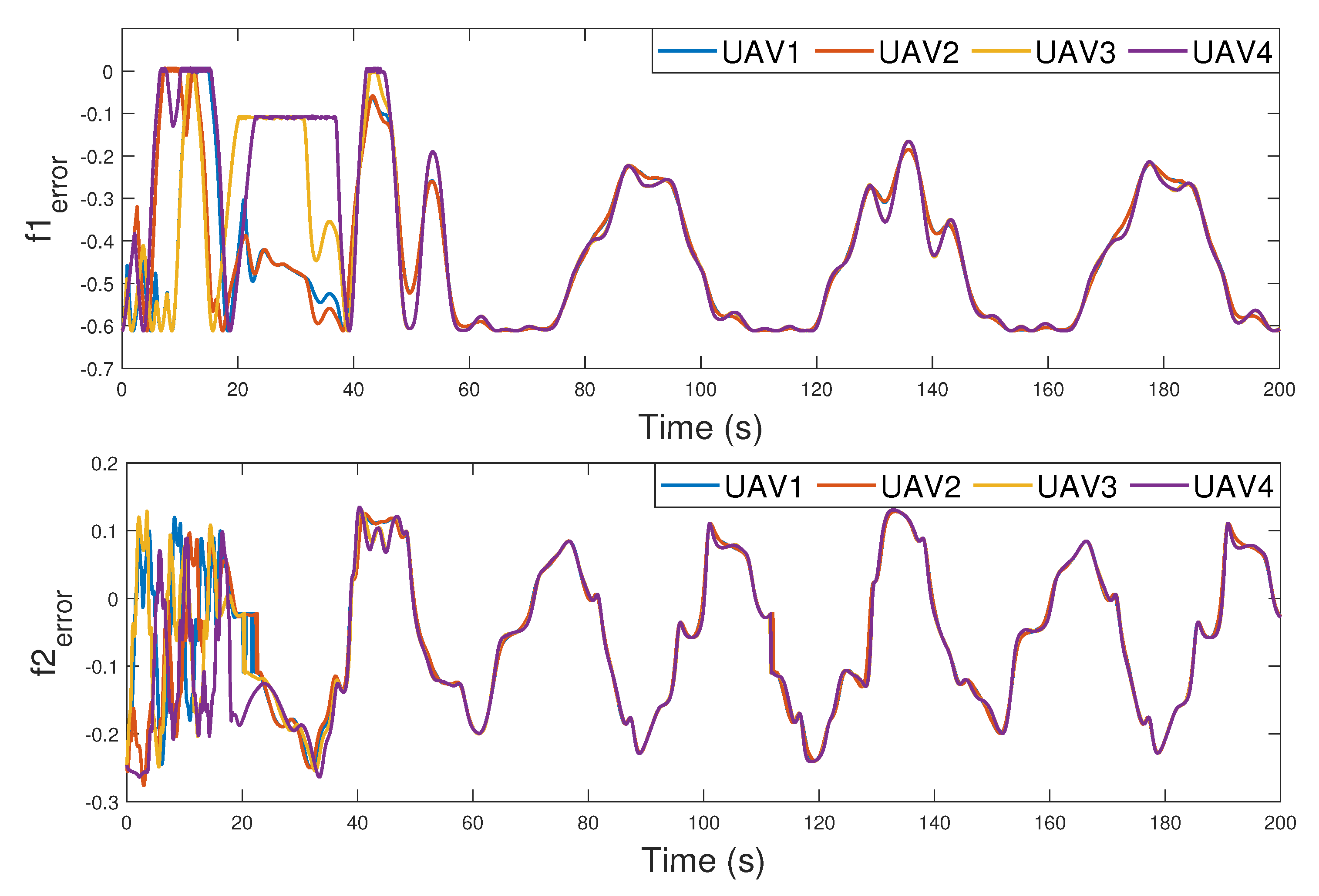
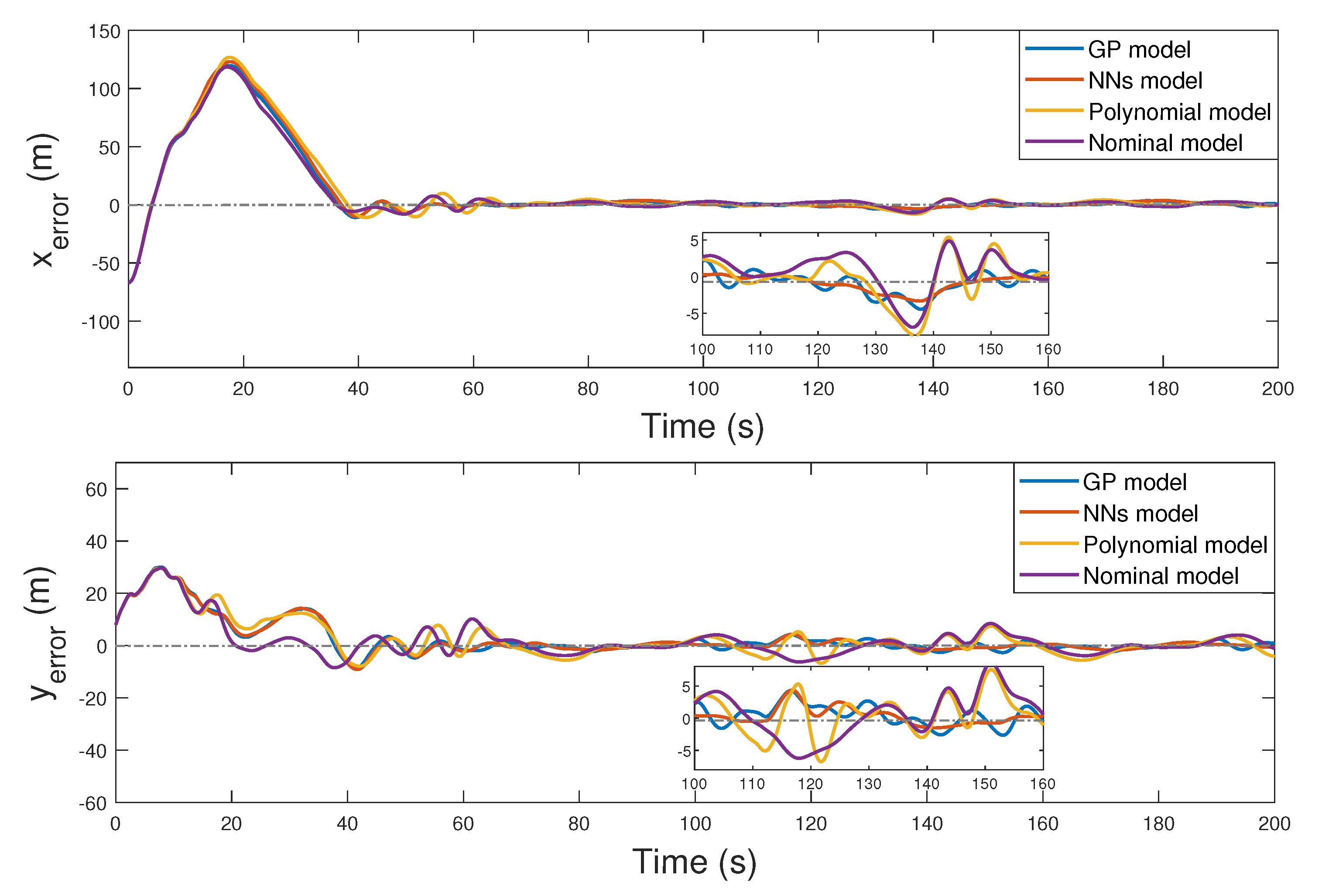
6. Simulation Results

In this section, we consider a simulation scenario that four UAVs track the target vehicle in the predefined formation. The simulation is carried out on a personal computer, which has 6 CPU cores (Intel(R) Core(TM) i7-10750H CPU @ 2.60GHz), and the simulation environment is Matlab2020a. fitrap function is used for Gaussian process regression.

The unknown parts of dynamic function are given as follows

$$\begin{array}{c}{f}_{i1}\left({\upsilon }_i,{\theta }_i\right)=-0.0035|{\upsilon }_i-13|exp\left(\sqrt{0.8{\upsilon }_i}\right),\hfill \\ f_{i2}\left({\upsilon }_i,{\theta }_i\right)=-0.04\sqrt{{\upsilon }_i}sin3{\theta }_i+\frac{ln{\upsilon }_i}{{\upsilon }_i^{1.5}}cos2{\theta }_i,\hfill \end{array}$$

(29)

where $i=1,2,3,4$. The 2500 training inputs are equally distributed on the set $[8,20]\times [-\pi ,\pi ]$, since the velocity of the UAV is subject to some constraints. The labels in the training pairs are the observed value of Equation (29) with Gaussian noise $\varsigma$, $\varsigma \sim \mathcal{N}(0,0.03)$.

The parts of disturbance, $d_{i1}$ and $d_{i2}$, are given as the white noise and bounded noise, respectively, which account for $2\%$ of control input. The trajectory of the target vehicle is given as follows

$$\begin{array}{c}{x}_0\left(t\right)=200cos0.07t,\hfill \\ y_0\left(t\right)=150sin0.07t,\hfill \end{array}$$

(30)

where $(x_0,y_0)$ is the position of the target vehicle.

Figure 3 shows interactions among the UAVs and the target vehicle, which is chosen under Assumption 1. The control gains are chosen to be $k_1=1.5,k_2=0.5$, the diagonal matrix $\mathit{B}=diag\{1,1,0,0\}$, the adjacency matrix $\mathit{A}$ and matrix $\tilde{\mathit{L}}$ are given as follows

$$\mathit{A}=\left[\begin{array}{cccc}0& 1& 0& 1\\ 1& 0& 1& 0\\ 0& 1& 0& 1\\ 1& 0& 1& 0\end{array}\right], \tilde{\mathit{L}}=\left[\begin{array}{cccc}3& -1& 0& -1\\ -1& 3& -1& 0\\ 0& -1& 2& 1\\ -1& 0& -1& 2\end{array}\right].$$

The whole simulation lasts for 200 seconds, during the simulation, the estimation error of GP model is bounded, which can be seen in Figure 4. It is noting that Gaussian noise $\varsigma$ is of great importance in the data learning of GP model, since too much noise would reduce the reliability of the training data.

To visually demonstrate the tracking performance, Figure 5 shows the trajectory of four UAVs and the target in the three-dimensional plots, where all UAVs track the target vehicle in the predefined formation. Figure 6 illustrates the consensus tracking error of each UAV, which is defined in Equation (19). It is noting that the consensus tracking error of each UAV converges to a certain bound exponentially and the final bounds of error in two directions are 1 m.

To show the effectiveness of the proposed method, we consider the other three cases, which include the case based on NNs model, based on polynomial model and based on nominal model. We employ a two-layer feed-forward network via Neural Net Fitting APP in Matlab to train NNs model of unknown dynamic, and the number of hidden neurons is 5 in the training. The polynomial model is trained via Curve Fitting APP in Matlab, and the degree of the polynomial is 3.

Table 1. The RMSE of three models.

	${\mathit{f}}_{\mathit{i}1}$	${\mathit{f}}_{\mathit{i}2}$
GP model	$0.0285$	$1.2407e-04$
NNs model	$0.0471$	$0.0232$
Polynomial model	$0.05425$	$0.9851$

demonstrates the RMSE of three models, among which the RMSE of GP model is minimal. Figure 7 shows the accumulated consensus tracking errors of 4 UAVs, which are defined as ${\sum }_{i=1}^4{\mathbf{\epsilon }}_{i,j}$, where $j=1,2$ denotes two directions. We can find that the tracking performance based on GP model and NNs model are almost the same, which are better than that based on polynomial model. The performance based on nominal model, without considering uncertainty, is the worst. Although the performance based on GP model and NNs model are almost the same, the uniform error of GP model can be explained based on Lemma 3.

7. Conclusions and Future Work

In this paper, we study a tracking problem of fixed-wing UAVs with uncertain dynamic. A group of UAVs needs to track the target vehicle in a predefined formation. We first establish the data-driven model for uncertain dynamic with the technique of Gaussian process regression. With the help of the main theorem proposed by Armin Lederer [17], the uniform error of the model is guaranteed to be bounded with a high probability. Then, we design a consensus protocol for the tracking control of multi-UAVs, where the bounded disturbance is considered. The stability of the system is proven via Lyapunov analysis, and the tracking error is guaranteed to be uniform bounded with a high probability. Finally, we carry out the numerical simulation. In the simulation scenario, we compare four cases, including the case based on NNs model, based on polynomial model and based on nominal model. The results demonstrate that the proposed method is effective and robust.

References

- Wang, X.; Shen, L.; Liu, Z.; Zhao, S.; Cong, Y.; Li, Z.; Jia, S.; Chen, H.; Yu, Y.; Chang, Y.; et al. Coordinated flight control of miniature fixed-wing UAV swarms: Methods and experiments. Sci. China Inf. Sci. 2019, 62, 1–17. [Google Scholar] [CrossRef] [Green Version]
- Wang, X.; Zeng, Z.; Cong, Y. Multi-agent distributed coordination control: Developments and directions via graph viewpoint. Neurocomputing 2016, 199, 204–218. [Google Scholar] [CrossRef]
- Nichols, J.W.; Sun, L.; Beard, R.W.; McLain, T. Aerial rendezvous of small unmanned aircraft using a passive towed cable system. J. Guid. Control Dyn. 2014, 37, 1131–1142. [Google Scholar] [CrossRef] [Green Version]
- Lellis, E.D.; Vito, V.D.; Ruby, M.; Salbego, N. Adaptive Algorithm for Fixed Wing Uav Autolanding on Aircraft Carrier, AIAA. 2013. Available online: https://arc.aiaa.org/doi/abs/10.2514/6.2013-4585 (accessed on 15 August 2013).
- Zhao, S.; Wang, X.; Chen, H.; Wang, Y. Cooperative Path Following Control of Fixed-wing Unmanned Aerial Vehicles with Collision Avoidance. J. Intell. Robot. Syst. 2020, 100, 1569–1581. [Google Scholar] [CrossRef]
- Gerardo, F.; Alejandro, F.; Andre, M. A full controller for a fixed-wing UAV. arXiv 2019, arXiv:1903.03945. Available online: https://arxiv.org/abs/1903.03945 (accessed on 10 March 2019).
- Su, C.; Wang, X.; Shen, L.; Yu, H. Adaptive uav maneuvering control system based on dynamic inversion and long-short-term memory network. In Proceedings of the 2020 Chinese Automation Congress (CAC), Shanghai, China, 6–8 November 2020; pp. 6880–6885. [Google Scholar]
- Ghommam, J.; Saad, M. Coordinated 3d path following control for a team of uavs with reference velocity recovery. In Proceedings of the 2009 European Control Conference (ECC), Budapest, Hungary, 23–26 August 2009; pp. 3008–3014. [Google Scholar]
- Tang, Y.; Lin, D.; Cao, L.J.; Liu, Y.C. Attitude Control of Fixed-Wing UAV Under Model Uncertainty and Disturbances. Electron. Opt. Control 2020, 27, 85–89. [Google Scholar]
- Roza, A.; Maggiore, M.; Scardovi, L. A smooth distributed feedback for formation control of unicycles. IEEE Trans. Autom. Control 2019, 64, 4998–5011. [Google Scholar] [CrossRef]
- Seyboth, G.S.; Wu, J.; Qin, J.; Yu, C.; Allgower, F. Collective circular motion of unicycle type vehicles with nonidentical constant velocities. IEEE Trans. Control Netw. Syst. 2014, 1, 167–176. [Google Scholar] [CrossRef]
- Hemakumara, P.; Sukkarieh, S. Non-parametric uav system identification with dependent gaussian processes. In Proceedings of the 2011 IEEE International Conference on Robotics and Automation, Shanghai, China, 9–13 May 2011; pp. 4435–4441. [Google Scholar]
- Beckers, T.; Umlauft, J.; Hirche, S. Stable model-based control with gaussian process regression for robot manipulators. IFAC-PapersOnLine 2017, 50, 3877–3884. [Google Scholar] [CrossRef]
- Maiworm, M.; Limon, D.; Findeisen, R. Online learning-based model predictive control with gaussian process models and stability guarantees. Int. J. Robust Nonlinear Control 2021. Available online: https://doi.org/10.1002/rnc.5361 (accessed on 27 September 2021).
- Deisenroth, M.P.; Fox, D.; Rasmussen, C.E. Gaussian processes for data-efficient learning in robotics and contro. IEEE Trans. Pattern Anal. Mach. Intell. 2015, 37, 408–423. [Google Scholar] [CrossRef] [Green Version]
- Srinivas, N.; Krause, A.; Kakade, S.M.; Seeger, M.W. Information-theoretic regret bounds for gaussian process optimization in the bandit setting. IEEE Trans. Inf. Theory 2012, 58, 3250–3265. [Google Scholar] [CrossRef] [Green Version]
- Lederer, A.; Umlauft, J.; Hirche, S. Uniform error bounds for gaussian process regression with application to safe control. In Proceedings of the 33rd Annual Conference on Neural Information Processing Systems, Vancouver, BC, Canada, 8–14 December 2019. [Google Scholar]
- Yang, Z.; Sosnowski, S.; Liu, Q.; Jiao, J.; Lederer, A.; Hirche, S. Distributed learning consensus control for unknown nonlinear multi-agent systems based on gaussian processes. arXiv 2021, arXiv:2103.15929. Available online: https://arxiv.org/abs/2103.15929 (accessed on 27 September 2021).
- O’Callaghan, S.; Ramos, F.T.; Durrant-Whyte, H. Contextual Occupancy Maps using Gaussian Processes. In Proceedings of the 2009 IEEE International Conference on Robotics and Automation, Kobe, Japan, 12–17 May 2009. [Google Scholar]
- Khansari-Zadeh; Kim, H.J.; Johansson, K.H. Path planning for remotely controlled UAVs using Gaussian process filter. In Proceedings of the 2017 17th International Conference on Control, Automation and Systems (ICCAS 2017), Jeju, Korea, 18–21 October 2017. [Google Scholar]
- Cai, L.; Liu, X.; Ding, H.; Chen, F. Human Action Recognition Using Improved Sparse Gaussian Process Latent Variable Model and Hidden Conditional Random Filed. IEEE Access 2018, 6, 20047–20057. [Google Scholar] [CrossRef]
- Ghasrodashti, E.K.; Helfroush, M.S.; Danyali, H. Sparse-Based Classification of Hyperspectral Images Using Extended Hidden Markov Random Fields. IEEE J. Sel. Top. Appl. Earth Obs. Remote Sens. 2018, 11, 4101–4112. [Google Scholar] [CrossRef]
- Kordi Ghasrodashti, E.; Helfroush, M.S.; Danyali, H. Spectral-spatial classification of hyperspectral images using wavelet transform and hidden Markov random fields. Geocarto Int. 2018, 33, 771–790. [Google Scholar] [CrossRef]
- Lee, J.; Muskardin, T.; Paez, C.R.; Oettershagen, P.; Stastny, T.; Sa, I. Roland Siegwart and Konstantin Kondak, Towards Autonomous Stratospheric Flight: A Generic Global System Identification Framework for Fixed-Wing Platforms. In Proceedings of the 2018 IEEE/RSJ International Conference on Intelligent Robots and Systems (IROS), Madrid, Spain, 1–5 October 2018. [Google Scholar]
- Yoo, J.; Mohammad, S.; Billard, A. Learning Stable Nonlinear Dynamical Systems With Gaussian Mixture Models. IEEE Trans. Robot. 2011, 27, 943–957. [Google Scholar]
- Hemakumara, P.; Sukkarieh, S. Learning UAV Stability and Control Derivatives Using Gaussian Processes. IEEE Trans. Robot. 2013, 29, 813–824. [Google Scholar] [CrossRef]
- Park, S.; Mustafa, S.K.; Shimada, K. Learning-Based Robot Control with Localized Sparse Online Gaussian Process. In Proceedings of the 2013 IEEE/RSJ International Conference on Intelligent Robots and Systems (IROS), Tokyo, Japan, 3–7 November 2013. [Google Scholar]
- Umlauft, J.; Pohler, L.; Hirche, S. An uncertainty-based control lyapunov approach for control-affine systems modeled by gaussian process. IEEE Control Syst. Lett. 2018, 2, 483–488. [Google Scholar] [CrossRef]
- Maiworm, M.; Limon, D.; Manzano, J.M.; Findeisen, R. Stability of gaussian process learning based output feedback model predictive control. In Proceedings of the 6th IFAC Conference on Nonlinear Model Predictive Control NMPC 2018, Madison, WI, USA, 19–22 August 2018; pp. 455–461. [Google Scholar]
- Wang, P.; Luo, Y.; Yu, J.J. Coordinated Formation for multiple UAVs Based on H∞ Control, 2020. (In Chinese). Available online: http://qikan.cqvip.com/Qikan/Article/Detail?id=7102783600 (accessed on 27 September 2021).
- Defoort, M.; Floquet, T.; Kokosy, A.; Perruquetti, W. Sliding-Mode Formation Control for Cooperative Autonomous Mobile Robots. IEEE Trans. Ind. Electron. 2008, 55, 3944–3953. [Google Scholar] [CrossRef] [Green Version]
- Ren, W.; Atkins, E. Distributed multi-vehicle coordinated controlvia local information exchange. Int. J. Robust Nonlinear Control 2007, 17, 1002–1033. [Google Scholar] [CrossRef] [Green Version]
- Rasmussen, C.E.; Williams, C.K.I. Gaussian Processes for Machine Learning; The MIT Press: Cambridge, MA, USA, 2006. [Google Scholar]
- Umlauft, J.; Beckers, T.; Kimmel, M.; Hirche, S. Feedback linearization using gaussian processes. In Proceedings of the 2017 IEEE 56th Annual Conference on Decision and Control (CDC), Melbourne, Australia, 12–15 December 2017; pp. 5249–5255. [Google Scholar]
- Beckers, T.; Colombo, L.; Hirche, S. Online learning-based trajectory tracking for underactuated vehicles with uncertain dynamics. arXiv 2020. Available online: https://arxiv.org/abs/2009.06689 (accessed on 27 September 2021).
- Ren, W. Consensus strategies for cooperative control of vehicle formations. IET Control Theory Appl. 2007, 1, 505–512. [Google Scholar] [CrossRef]