Multi-Mode Active Suspension Control Based on a Genetic K-Means Clustering Linear Quadratic Algorithm

Abstract

The traditional Linear quadratic regulator (LQR) control algorithm depends too much on expert experience during the selection of weighting coefficients. To solve this problem, we proposed a Genetic K-means clustering Linear quadratic (GKL) algorithm. Firstly, a 2-DOF 1/4 vehicle model and road input model are established. The weights of an LQR controller are optimized using a genetic algorithm. Then, a possible weighting space is constructed based on this optimal solution. Random weighting coefficients of each performance index are generated in this space. Next, LQR control for the 1/4 vehicle model is performed, and the simulation data are recorded automatically, with these random weighting values, different road classes, and driving speed. A machine learning dataset is built from these simulations. Finally, a K-means clustering algorithm is used to classify the LQR control active suspension into three performance modes: safety mode, comprehensive mode, and comfort mode. The optimal weighting matrix of each performance mode is determined to satisfy requirements for different types of drivers. The results show that the new GKL algorithm not only improves the suspension control effect but also realizes different performance modes. It can better adapt to the changes in driving conditions and drivers.

1. Introduction

The suspension is an important part of the vehicle chassis system, and its performance has a great influence on the handling stability, ride comfort, and driver’s driving experience. Compared with passive suspension, the active suspension has a better control effect in vibration. It can realize dynamic adaptive adjustments according to the driving conditions and ensure the suspension system is always in the best damping state, which significantly improves the ride comfort and handling stability of the vehicle. Therefore, the control algorithms of active suspension have become the research hotspot in the automotive industry. Many experts have conducted many studies on the algorithms, including adaptive PID control [1], fuzzy control [2], sliding mode control [3], neural networks [4], reinforcement learning [5], etc. Besides, the LQR theory, as one of the earliest and most mature control algorithms in modern control theory, has been studied deeply [6,7,8,9,10].

In the design of the LQR controller of active suspension, the design requirements of comfort, safety, and deflection conflict with each other. The selection of the weighting coefficients of the function indexes plays a very important role in suspension performance. Usually, multiple performance indexes are weighted to calculate an optimal solution. Therefore, how to select the weighting coefficients becomes the key in the design of the LQR controller. At present, many researchers realized that the traditional weights selection relies too much on the designer’s experience, so they have made many attempts to solve this subjective problem. Compared with the various analytic hierarchy process methods [11,12,13], genetic algorithm (GA) can eliminate more subjective components. Chen Shuang et al. [14] proposed a genetic particle swarm optimization algorithm by combining the advantages of the genetic algorithm and particle swarm optimization (PSO), which is used to optimize the weighting coefficients of performance indexes in the LQR control algorithm. Ranjan et al. [15] proposed an adaptive predator–prey optimization algorithm, which solved the problem of premature convergence of particles in PSO and the imbalance between the exploration and exploitation of particles in global optimization. In references [16,17], more genetic algorithms are applied to the optimal control of the active suspension. The weighting coefficients are searched in given weighting ranges by using the population search strategy and global search characteristics. The comprehensive performance of suspension is improved obviously by using these genetic algorithms. However, most of these algorithms have poor local search capability and may take quite a long time to run a globe searching. Li et al. [18] combined a qualitative analytic hierarchy process with GA to the LQR controller, which can increase the global optimization speed efficiently. Most of these PSO, GA, and other algorithms in references [14,15,16,17,18] adopt the idea of longitudinal iterative to find the optimal solution, so they must meet high requirements on iterative convergence. In addition, we can only obtain one unique solution from these algorithms, which obviously conflict with three compromised indexes.

More importantly, individual differences in driving styles are not considered in the above algorithms. Therefore, how to judge a driver’s feature and classify it into different modes are valuable. Many machine learning algorithms, even the simplest clustering approaches, have shown good applications on this topic. Constantinescu et al. [19] used a hierarchical clustering and a principal component analysis to identify and classify driving styles. In references [20,21,22], a K-means clustering algorithm was used to classify driving styles into normal type, soft type, and aggressive type. Although this above classification is aimed at the behaviors of longitudinal acceleration and deceleration, or the lateral lane-change maneuver, this classification idea, concentrating on the driver’s psychology, physiology, personality, and other human factors, is much valuable for suspension control. Therefore, proper clustering may provide a more accurate response for suspension control or be better adaptive to the drivers and roads. We may solve the conflict between the multi-indexes and the uniqueness of the solution by providing optimizations for each driving style.

Different from the longitudinal iteration principle, the clustering algorithm in machine learning is a horizontal algorithm, which could replace global optimization with local solutions. The popular K-mean clustering can classify objects effectively according to the correlation degree of attributes among objects [23,24]. This provides a new idea for solving the weighting coefficients of the LQR controller and designing the suspension control mode that adapts to the driving style. In references [20,21,22], data such as throttle open-angle and vehicle speed are used to classify drivers. Their datasets are collected from real vehicles. However, due to the lack of a commercial active suspension system, it is very hard for us to obtain the test data of a real suspension controller. Thus, it is necessary to explore a reasonable construction approach of the simulation dataset, generating enough suspension data to provide for the K-means clustering algorithm.

Therefore, a new Genetic K-means clustering Linear quadratic (GKL) algorithm for suspension classification control is proposed in this paper. At first, an optimal global solution of LQR control weighting coefficients is calculated using traditional GA. Then, according to this unique solution, a weighting space of suspension performance indexes is set up with variable scaling factors. Next, a Two-dimensional data points of $q_1$ and $q_2$ are randomly generated according to this newly designed weighting space. While changing the road class and driving speed, and the 1/4 vehicle model controlled by LQR is run for simulation. A machine learning dataset for the LQR active suspension is constructed. The dataset consists of 60 thousand points with 15 elements, including simulation results of three suspension indexes, among others. Finally, the simple K-means clustering algorithm is used to classify different suspension performance modes. For each mode, a locale optimal solution of the weighting coefficients is obtained. The simulation results show that these optimizations for three modes are adaptive to various driver types and improve the suspension responses in different driving conditions.

2. Active Suspension Systems and Control Systems

2.1. GKL Control Principle

In order to solve the above problems, a new GKL algorithm is proposed, and its principle is shown in Figure 1. The basic of suspension control is the traditional LQR algorithm on a 1/4 vehicle model. The control force is the K gain of the state vector by solving the Riccati equation. By aiming at a more objective weighting coefficients selection, a genetic algorithm program is used to search for a unique optimal solution for the comprehensive performances, shown in the top-right of Figure 1. A possible weighting space of $q_1$ and $q_2$ is constructed based on the scaling of this unique solution. Plenty of the active control simulations are carried out by randomly selecting weights within the weighting space and changing the road class and driving speed. Thus, a machine learning dataset for active suspension could be built with these input parameters and output indexes records. Finally, a K-mean clustering algorithm is used to classify the individual’s requirement on suspension performances into three modes, as shown in the left-bottom of Figure 1. A solution set of optimal weighting coefficients is offered for different types of drivers. Except for the integral optimal unique solution solved by GA, two new optimal solutions are provided in this set, which emphasizes more safety and comfort, respectively.

2.2. 2-DOF 1/4 Vehicle Model

The vehicle suspension dynamics model is the basis for suspension system design and performance analysis. In this paper, a 2-DOF 1/4 vehicle dynamics model is built, as shown in Figure 2.

Where $m_b$ and $m_w$ are the sprung mass and the unsprung mass, $K_s$ is the suspension stiffness, $K_t$ is the tire stiffness, $C_s$ is the suspension damping, $U_a$ is the active control force of suspension, when $U_a=0$, it is passive suspension.

According to the suspension model, the dynamic equation of the system is established by Newton’s law, which is:

$$m_b{\ddot{z}}_b=K_s(z_w-z_b)+C_s({\dot{z}}_w-{\dot{z}}_b)+U_a$$

(1)

$$m_w{\ddot{z}}_w=K_t(z_g-z_w)+C_s({\dot{z}}_b-{\dot{z}}_w)-K_s(z_w-z_b)-U_a$$

(2)

where $z_b$ is the vertical displacement of the car body, $z_w$ is the vertical displacement of the wheel, $z_g$ is the road displacement, ${\dot{z}}_b$ is the body vertical speed, ${\dot{z}}_w$ is the wheel vertical speed, ${\ddot{z}}_b$ is body vertical acceleration, and ${\ddot{z}}_w$ is the wheel vertical acceleration.

The vehicle model parameters are listed in

Table 1. Vehicle model parameters.

Model Parameter	Parameter Value	Model Parameter	Parameter Value
$m_b/\mathrm{kg}$	320	$C_s{/(\mathrm{N}·\mathrm{s}·\mathrm{m}}^{-1})$	1000
$m_w/\mathrm{kg}$	40	$n_0/\mathrm{Hz}$	0.1
$K_s/(\mathrm{N}·{\mathrm{m}}^{-1})$	22,000	$f_0/\mathrm{Hz}$	0.1
$K_t{/(\mathrm{N}·\mathrm{m}}^{-1})$	200,000	${u/(\mathrm{m}·\mathrm{s}}^{-1})$	20

.

2.3. Road Input Model

The road input model is the basis of the dynamic response and control of the vehicle, which is closely related to the suspension performance. Usually, the greater the road roughness is the worse the suspension performance responses.

For vehicles, most driving conditions can be regarded as random road inputs. Therefore, a filtered white noise of Gaussian distribution is used to generate the random road profile, and the time domain expression of road displacement is obtained:

$${\dot{z}}_g(t)=-2\pi f_0{z}_g(t)+2\pi n_0\sqrt{G_{0}u}w(t)$$

(3)

where $f_0$ is the lower cut-off frequency, and the value is 0.1 Hz; $n_0$ is the space reference frequency, and the value is 0.1 m⁻¹; $G_0$ is the road roughness coefficient; $u$ is the driving speed; $w$ is the Gaussian white noise with a mathematical expectation of zero; $z_g$ is the road displacement.

In the previous study of suspension control algorithms, the simulation and test are usually only carried out under a single road class. It is hard to describe the actual driving conditions in one simulation. Therefore, we establish a composite road model for active suspension controls.

A-class to D-class roads are recorded for 10 s in turn to build this composite road. The time domain response curve is shown in Figure 3.

2.4. LQG Controller Design of Active Suspension

The two main functions of the vehicle suspension are to ensure that the vehicle has good ride comfort and handling stability when driving. At the same time, the working space of suspension needs to be controlled within a certain range and meet the requirements of body posture during accelerating, decelerating, braking, or steering. Therefore, for the 2-DOF 1/4 vehicle suspension model, the three parameters of body vertical acceleration (BA), suspension working space (SWS), and dynamic tire deflection (DTD) are selected as performance indexes to quantitatively evaluate the suspension performance.

The state vector of the system is:

$$X={\left[\begin{array}{cc}{\dot{z}}_b& \begin{array}{cccc}{\dot{z}}_w& z_b& z_w& z_g\end{array}\end{array}\right]}^T$$

(4)

The output vector of the system is:

$$Y={\left[\begin{array}{ccc}{\ddot{z}}_b& z_b-z_w& z_w-z_g\end{array}\right]}^T$$

(5)

where ${\ddot{z}}_b$ is body vertical acceleration, $z_b-z_w$ is suspension working space, $z_w-z_g$ is dynamic tire deflection.

By combining Equations (1)–(3), and writing the system motion equation and the road input equation in the form of a matrix, the space state equation of the system can be obtained:

$$\dot{X}=AX+BU+FW$$

(6)

$$Y=CX+DU$$

(7)

where, $A=\left[\begin{array}{ccccc}-\frac{C_s}{m_b}& \frac{C_s}{m_b}& -\frac{K_s}{m_b}& \frac{K_s}{m_b}& 0\\ \frac{C_s}{m_w}& -\frac{C_s}{m_w}& \frac{K_s}{m_w}& \frac{-K_t-K_s}{m_b}& \frac{K_t}{m_w}\\ 1& 0& 0& 0& 0\\ 0& 1& 0& 0& 0\\ 0& 0& 1& 0& -2\pi f_0\end{array}\right]$, $B=\left[\begin{array}{c}\frac{1}{m_b}\\ -\frac{1}{m_w}\\ 0\\ 0\\ 0\end{array}\right]$, $F=\left[\begin{array}{c}0\\ 0\\ 0\\ 0\\ 2\pi n_0\sqrt{G_{0}u}\end{array}\right]$, $C=\left[\begin{array}{ccccc}-\frac{C_s}{m_b}& \frac{C_s}{m_b}& -\frac{K_s}{m_b}& \frac{K_s}{m_b}& 0\\ 0& 0& 1& -1& 0\\ 0& 0& 0& 1& -1\end{array}\right]$, $D=\left[\begin{array}{c}\frac{1}{m_b}\\ 0\\ 0\end{array}\right]$.

where $A$ is the state matrix of the system, $B$ is the input matrix of the control vector, $F$ is the road input matrix, $C$ is the output matrix, $D$ is the transfer matrix, $U=\left[U_a(t)\right]$ is the control input matrix of active suspension, and $W=\left[w(t)\right]$ is the gaussian white noise input matrix.

The comprehensive index J of the LQR controller is defined with the three performance indexes as follows:

$$J=\underset{T\to \infty }{{\displaystyle \lim }}\frac{1}{T}{\displaystyle {\int }_0^T[q_1{(z_w(t)-z_g(t))}^2}+q_2{(z_b(t)-z_w(t))}^2+q_3{\ddot{z}}_b(t)]dt$$

(8)

where, $q_1$, $q_2$, and $q_3$ are the weighting coefficient of DTD, SWS, and BA. The selection of the weighting coefficient reflects the designer’s tendency towards different performances. Due to these three weights essentially representing the relative values among them, the weighting coefficient $q_3$ of BA is usually set to 1 for the convenience of calculation.

Rewrite the above expression (8) into a matrix form:

$$J=\underset{T\to \infty }{\lim }\frac{1}{T}{\displaystyle {\int }_0^T(X^{T}QX+U^{T}RU+2X^{T}NU)dt}$$

(9)

where, $Q=\left[\begin{array}{ccccc}\frac{C_s^2}{m_b^2}& -\frac{C_s^2}{m_b^2}& \frac{C_s{K}_s}{m_b^2}& -\frac{C_s{K}_s}{m_b^2}& 0\\ -\frac{C_s^2}{m_b^2}& \frac{C_s^2}{m_b^2}& -\frac{C_s{K}_s}{m_b^2}& \frac{C_s{K}_s}{m_b^2}& 0\\ \frac{C_s{K}_s}{m_b^2}& -\frac{C_s{K}_s}{m_b^2}& \frac{K_s^2}{m_b^2}+q_2& -\frac{K_s^2}{m_b^2}-q_2& 0\\ -\frac{C_s{K}_s}{m_b^2}& \frac{C_s{K}_s}{m_b^2}& -\frac{K_s^2}{m_b^2}-q_2& \frac{K_s^2}{m_b^2}+q_2+q_1& -q_1\\ 0& 0& 0& -q_1& q_1\end{array}\right]$, $R=\frac{1}{m_b^2}$, $N=\frac{1}{m_b^2}\left[\begin{array}{c}-C_s\\ C_s\\ -K_s\\ K_s\\ 0\end{array}\right]$.

where Q is the weighting matrix of state variables, R is the weighting matrix of control variables, and N is the weighting coefficient of cross terms.

When vehicle parameters and weighting coefficients values are determined, the optimal control feedback gain matrix can be solved by the Riccati equation, and its form is as follows:

$$PA+A^{T}P-(PB+N)R^{-1}(B^{T}P+N^T)+Q=0$$

(10)

The optimal control feedback gain matrix is determined by vehicle parameters and weighting coefficients, and its form is as follows:

$$K=R^{-1}(B^{T}P+N^T)$$

(11)

The optimal control force $U_a$ at time t can be calculated as the negative gain of the state vector:

$$U_a(t)=-KX(t)$$

(12)

3. GA Optimization on LQR Weighting Coefficients

According to the LQR control principle, the optimal solution of the controlled system depends on the selection of weighting matrix Q and R. However, these two matrixes cannot be solved by an analytic method. These matrix parameters can only be selected qualitatively, which makes the selection of weights of the LQR controller more subjective and dependent too much on the designer’s experience. Additionally, if the selection of Q and R is not appropriate, the optimal solution would have no practical significance and application value.

GA is a global search algorithm developed by imitating the mechanism of biological evolution, which is based on natural selection and genetic theory. This algorithm adopts the principle of survival of the fittest, elimination of inferior. In the iterative process, the population evolves towards the optimal direction through the steps of selection, crossover, and mutation and finally obtains the optimal solution that meets the requirements. Therefore, we applied GA to optimize the LQR controller of active suspension and take the solution as the reference value for the weighting space construction in our GKL algorithm.

3.1. Genetic Algorithm

Due to the orders of magnitude and units of the three performance indexes of suspension being different, it needs a normalization comparison. The root mean square (RMS) values of three active suspension performance indexes are divided by their corresponding RMS value of the passive suspension and then added together as a fitness function of GA:

$$\min L=\frac{rmsB{A}_a}{rmsB{A}_p}+\frac{rmsSW{S}_a}{rmsSW{S}_p}+\frac{rmsDT{D}_a}{rmsDT{D}_p}$$

(13)

where $rmsB{A}_a$, $rmsSW{S}_a$, $rmsDT{D}_a$ are the RMS values of BA, SWS, DTD of active suspension; $rmsB{A}_p$, $rmsSW{S}_p$, $rmsDT{D}_p$ are the RMS values of BA, SWS, DTD of passive suspension.

The constraint conditions are:

$$s.t.\{\begin{array}{l}rmsB{A}_a<rmsB{A}_p\\ rmsSW{S}_a<rmsSW{S}_p\\ rmsDT{D}_a<rmsDT{D}_p\end{array}$$

(14)

The optimization process of GA is shown in Figure 4. Additionally, the steps are as follows:

• Generate initial population of weighting coefficients;
• The values of individuals in the population are assigned to the weighting coefficients $q_1$, $q_2$, and $q_3$ of the LQR controller in turn. The optimal gain feedback matrix $K$ is solved by Riccati Equation (10), and then the optimal control force $U_a(t)$ is solved by Formula (12). Then the control force is acted on the active suspension model, and the RMS values of the three performance indexes are calculated;
• On the premise that the constraint conditions (14) are satisfied, the fitness function value of each individual in the population is calculated by the Formula (13). If the termination condition is met, the GA is exited, and the optimal individual value is returned; if not, it is transferred to step 4;
• GA continues with selection, crossover, and mutation to produce a new population and then proceeds to step 2 to repeat the cycle until the termination conditions are met and exit the cycle.

3.2. Simulation Analysis

In the optimization process of GA, to guarantee the control effect of BA and reduce the number of iterations, the weighting coefficient of BA is set to 1. We took the optimization results of the literature [14] as references and expanded the range of weighting coefficients $q_1$ and $q_2$ intervals as larger as possible to ensure the reliability of the optimization search results. For GA, the main parameters are the population size, the number of interactions, the crossover fraction, and the mutation fraction. We set these parameters of GA using the values set in the literature [16,17] as references. As can be seen from Figure 5a, the value of the fitness function has reached the optimum at the 12th iterations. Therefore, it is sufficient to set the generations and termination generation to 20. Furthermore, the selection of crossover fraction and the genetic fraction is crucial to the performance of genetic algorithms. The larger the crossover fraction, the faster new individuals are generated. However, when the crossover fraction is too large, there is a possibility of the genetic pattern being destroyed, making the structure of individuals with high fitness destroyed. Additionally, if the crossover fraction is too small, the search process is slow, and the search time is prolonged. For the mutation fraction, if its value is too small, it is not easy to generate new individuals. If the mutation fraction is too large, the randomness of the genetic algorithm search is too large. Therefore, we used the values in the literature [16,17] as references, and the two parameters were fine-tuned to simulation. Finally, the crossover fraction is set to 0.4 and the mutation fraction to 0.05. The parameters of the GA are shown in

Table 2. Parameters of GA.

Model Parameter	Value	Model Parameter	Value
Search interval of $q_1$	(0, 2 × 105)	Crossover fraction	0.4
Search interval of $q_2$	(0, 2 × 104)	Generations	20
Population size	100	Termination generation	20
Elite count	10	Fitness function deviation value	1 × 10−4
Mutation fraction	0.05

.

The variation in fitness function value is shown in Figure 5a. The optimal solution of weighting coefficients is shown in Figure 5b.

From the simulation results in Figure 5, it can be seen that the fitness function value is optimized with the population evolving and finally converges to 2.42819. The weighting coefficients’ optimal solution is: $q_1=68680$, $q_2=9259$, $q_3=1$.

Simulations are performed when the road input is the A-class to D-class composite road, simulation speed is 20 m/s, and simulation time is 40 s. The time domain curves of 1/4 vehicle model’s BA, SWS, and DTD are obtained, as shown in Figure 6a–d.

In Figure 6, the solid lines are the results of a passive suspension, and the dot–dash lines are those for active control. Compared with passive suspension, the vibration range of each performance index is reduced after the optimization and control. To quantitatively describe the improvement effect, the RMS values and improvement rate of each performance index are calculated, as shown in

Table 3. RMS values and improvement rate of suspension performance indexes.

Road Class	Suspension Type	RMS Values
		BA	SWS	DTD
A	Passive	0.3377	0.0034	0.0011
	GA-LQR	0.2900	0.0023	0.0010
	Improvement/%	−14.14% 1	−32.94%	−7.30%
B	Passive	0.6755	0.0068	0.0023
	GA-LQR	0.5780	0.0043	0.0021
	Improvement/%	−14.44%	−36.62%	−7.32%
C	Passive	1.3526	0.0135	0.0045
	GA-LQR	1.1616	0.0091	0.0041
	Improvement/%	−14.12%	−32.94%	−7.19%
D	Passive	2.7168	0.0271	0.0093
	GA-LQR	2.3298	0.0182	0.0086
	Improvement/%	−14.25%	−32.87%	−7.58%

¹ The negative changing rate represents optimization, and the positive changing rate represents deterioration.

.

Comparing the RMS values in Table 3, we can find that the BA decreases about 14%, which effectively refines the comfort for the driver; the improvement rate of SWS is about 34%, which can ensure the working space of suspension meets the requirements of the space structure; the optimization rate of DTD is about 7.3%, which guarantee the tire adhesion for safety. In summary, the LQR controller optimized by GA has significantly improved the comprehensive performance of the vehicle.

4. GKL Algorithm of Active Suspension

The GA mentioned in the previous section can only obtain one optimal solution for the LQR controller. The adaptability to variable working conditions is poor. It cannot meet the different requirements of different drivers for vehicle performance either. Therefore, in this paper, we introduce a machine learning approach to solve these problems.

4.1. Active Suspension Machine Learning Dataset

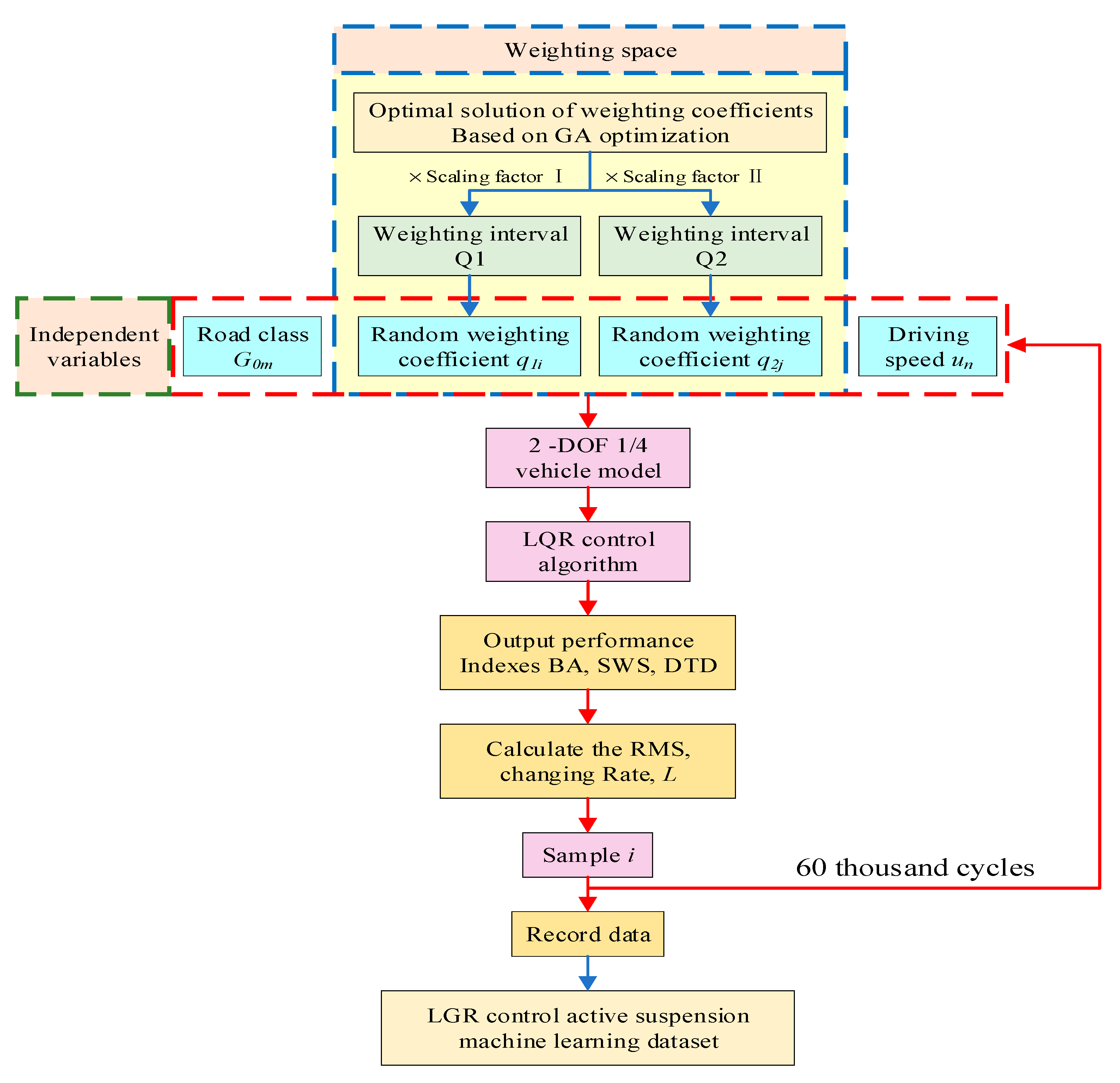
The performance of vehicle suspension is affected by many factors, which can be divided into internal and external factors. In terms of the internal factors, according to the LQR control principle, the selection of weighting coefficients has a great influence on the control effect. In terms of the external factors, the performance of suspension is affected by road roughness and vehicle motion state. Therefore, we take these two kinds of factors into account together. We selected five factors, including road class, vehicle speed $u$, DTD weighting coefficient $q_1$, SWS weighting coefficient $q_2$, and BA weighting coefficient $q_3$ as independent variables to carry out simulations and build the machine learning dataset of LQR control active suspension.

In the sample simulation, the BA weighting coefficient $q_3$ is set as 1 for simplification, and the other four factors are selected as independent variables. The construction process of the machine learning dataset is shown in Figure 7.

• Generate random numbers

A possible weighting space is constructed based on the optimal solution optimized by GA. Two scaling factors, 1.75 and 1.1 in this case, are used to limit the range of weighting coefficients $q_1$ and $q_2$, that is $q_1\in \left[0,120000\right]$, $q_2\in \left[0,10000\right]$. Then, 50 random numbers are generated in their respective intervals to form 2500 combinations of the weights. The random numbers are generated with the Linear congruential method as follows.

Generate random seeds:

$$S_0=seed;$$

(15)

Generate random numbers:

$$S_{i+1}=a{S}_n+b[MOD(M)]$$

(16)

where A, B, and M are integer constants, MOD is the remainder operation.

The generated Two-dimensional random data points, $(q_{1i},q_{2j})$ in this case, are listed in

Table 4. Two-dimensional random data points $(q_{1i},q_{2j})$.

Parameters	Values
$q_{1i}$	3738	5703	7397	7440	8461	13,050	14,934	18,738	20,772	23,063
	23,571	29,017	31,616	34,455	34,885	41,372	41,987	45,985	46,489	46,568
	53,650	57,407	58,815	60,134	65,260	69,988	72,053	75,262	76,333	78,009
	80,244	81,324	81,546	82,576	83,398	83,887	83,932	84,101	87,958	89,062
	91,815	92,447	93,655	95,776	108,877	110,035	110,872	111,768	113,821	119,888
$q_{2j}$	322	425	1021	1119	1945	2222	2261	2619	2620	2853
	2869	2963	3957	4269	4375	4478	4675	4945	5078	5154
	5183	5230	5417	5518	5585	5601	5645	5803	6948	7264
	7283	7311	7327	7447	7588	7594	7604	8140	8254	8551
	8616	8796	9041	9059	9213	9229	9460	9549	9950	9974

;

2.

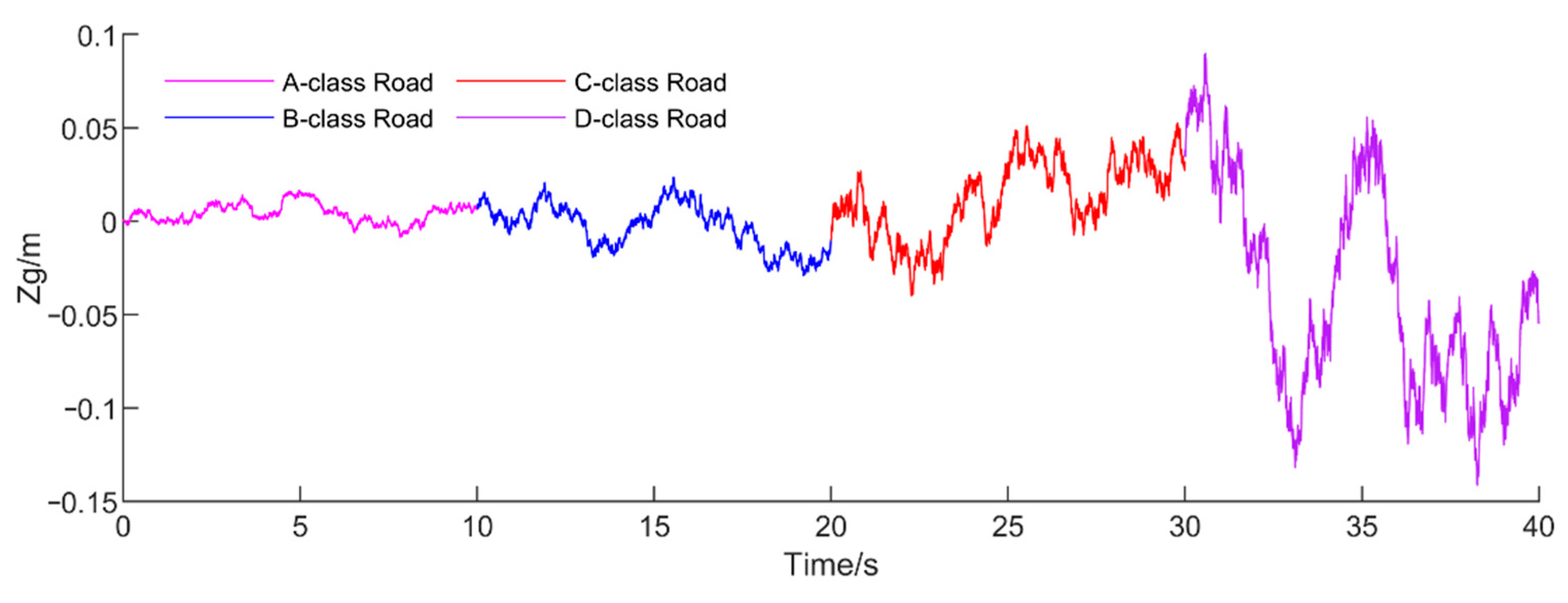
Select road class

According to the ride comfort test standards of passenger cars (ISO2631-1), the road roughness coefficient $G_0$ of four road classes (A, B, C, and D) is selected in turn;

3.

Select driving speed

Select six driving speeds (5, 10, 15, 20, 25, and 30 m/s) in turn;

4.

Select the weighting coefficients of performance indexes

Select the weights $q_1$ and $q_2$ of DTD and SWS in turn;

5.

Model simulation

After all independent variables have been selected, the 1/4 vehicle model is run for simulation;

6.

Construct the machine learning dataset of LQR active suspension

The results of each simulation are output and saved in the form of a matrix to construct the machine learning dataset of LQR active suspension (4 × 6 × 50 × 50 = 60,000 samples in total).

Each machine learning sample point contains 15 elements, including road roughness coefficient $G_0$, driving speed $u$, three weighting coefficients of performance indexes, three performance RMS values for active control and three for passive suspension, three changing rates of the performances, and the suspension integral control effect index $L$.

The sample vector $Sample i$ is as follows:

$$Sample i=\left[\begin{array}{ccccccccccccccc}{G}_0& u& q_1& q_2& q_3& rmsB{A}_a& rmsSW{S}_a& rmsDT{D}_a& rmsB{A}_p& rmsSW{S}_p& rmsDT{D}_p& dBA& dSWS& dDTD& L\end{array}\right]$$

(17)

The changing rate of three performance indexes are as follows:

$$dBA=\frac{rmsB{A}_a-rmsB{A}_p}{rmsB{A}_p}$$

(18)

$$dSWS=\frac{rmsSW{S}_a-rmsSW{S}_p}{rmsSW{S}_p}$$

(19)

$$dDTD=\frac{rmsDT{D}_a-rmsDT{D}_p}{rmsDT{D}_p}$$

(20)

where $dBA$, $dSWS$, $dDTD$ are the changing rate of BA, SWS, DTD.

The suspension integral control effect index $L$ is as follows:

$$L=\frac{rmsB{A}_a}{rmsB{A}_p}+\frac{rmsSW{S}_a}{rmsSW{S}_p}+\frac{rmsDT{D}_a}{rmsDT{D}_p}$$

(21)

4.2. Data Analysis Based on K-means Clustering Algorithm

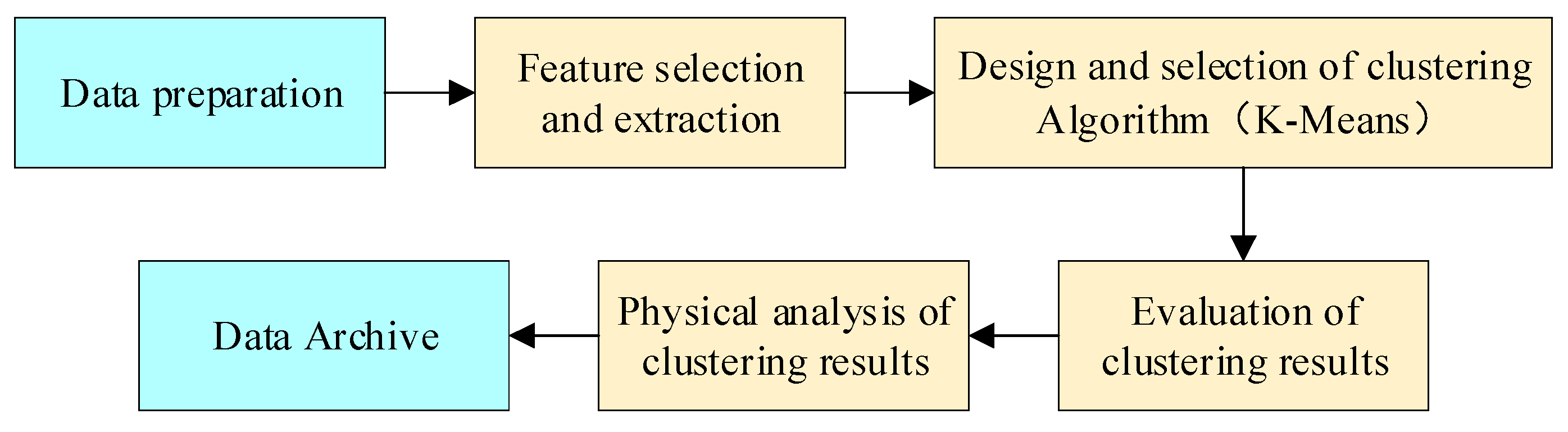
Clustering analysis is one of the popular algorithms in machine learning algorithms; it has the advantages of simplicity, practicality, and efficiency. Therefore, we chose a cluster analysis to analyze the data of the machine learning dataset constructed in the previous section. The cluster analysis process is shown in Figure 8, which mainly includes feature selection, clustering algorithm selection, clustering results evaluation, and physical analysis of clustering results.

4.2.1. Selection of Feature and Clustering Algorithm

Feature selection refers to the selection of several effective features from all the original features in the dataset to optimize the specific indexes of the system. Through a good feature selection, we can reduce the dimensions of the dataset and improve the efficiency of the machine learning algorithm. In this case, the RMS values of the three performance indexes of active suspension are chosen as the effective characteristics for clustering analysis.

K-means clustering algorithm [25] is subordinate to the partition clustering algorithm, which generally uses European distance as an index to measure the similarity between data objects. It has the advantages of simple process, fast operation speed, and good clustering effect. Therefore, we use the K-means clustering algorithm to analyze the machine learning dataset.

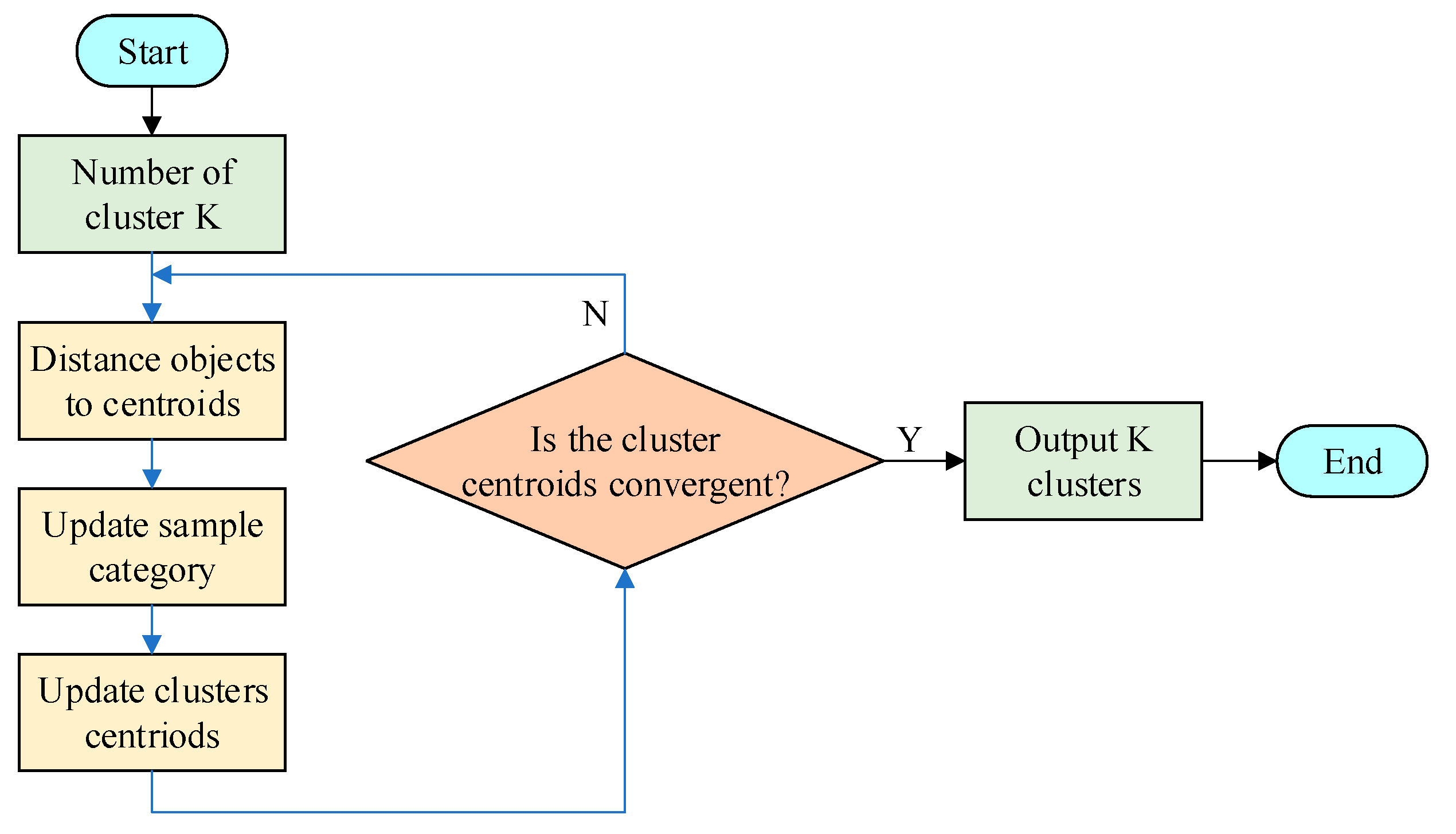
The process of the K-means clustering algorithm is shown in Figure 9:

• Initialization

K objects are randomly selected as the initial cluster centers;

2.

Set iteration termination conditions

The maximum number of cycles N or the sum of the squares of errors of the cluster center SSE are usually set as the termination conditions. The calculation formula of SSE is:

$$SSE={{\displaystyle \sum _{i=1}^K{\displaystyle \sum _{c\in C_i}\left|d(x,C_i)\right|}}}^2$$

(22)

where, $x$ is the data object, $C_i$ is ith cluster center, $K$ is the number of clusters;

3.

Update the cluster of the sample object

$$d(x,C_{{}^i})=\sqrt{{\displaystyle \sum _{j=1}^m{(x_j-C_i{}_j)}^2}}$$

(23)

where $m$ is the dimension of the data object, $x_j$ and $C_{ij}$ are the jth attribute values of $x$ and $C_i$.

The Euclidean distance $d_{ij}$ of each data object to the cluster center $C_i$ is calculated by Equation (23), and the data object is allocated to the cluster close to the $C_i$ according to the distance criterion;

4.

Update the center of the cluster

$$u_i=\frac{1}{\left|C_i\right|}{\displaystyle \sum _{x\in C_i}x}$$

(24)

where $u_i$ is the new cluster center.

The new cluster center $u_i$ is recalculated for all sample points in $C_i$ by formula (24);

5.

Repeat steps 3 to 4 until the termination conditions in step 2 are met. Then, the iteration is stopped, and the clustering is completed.

4.2.2. Evaluation of Clustering Results

The active suspension LQR controller studied in this paper changes 4 kinds of road classes, 6 kinds of speed, 50 weighting coefficients of DTD, and 50 weighting coefficients of SWS. The sample data of the machine learning dataset constructed after the simulation are so large that the clustering analysis cannot be carried out directly. Thus, keeping the road class and driving speed unchanged, a control variable method is used to divide the dataset into 24 subsets (i.e., 24 working conditions).

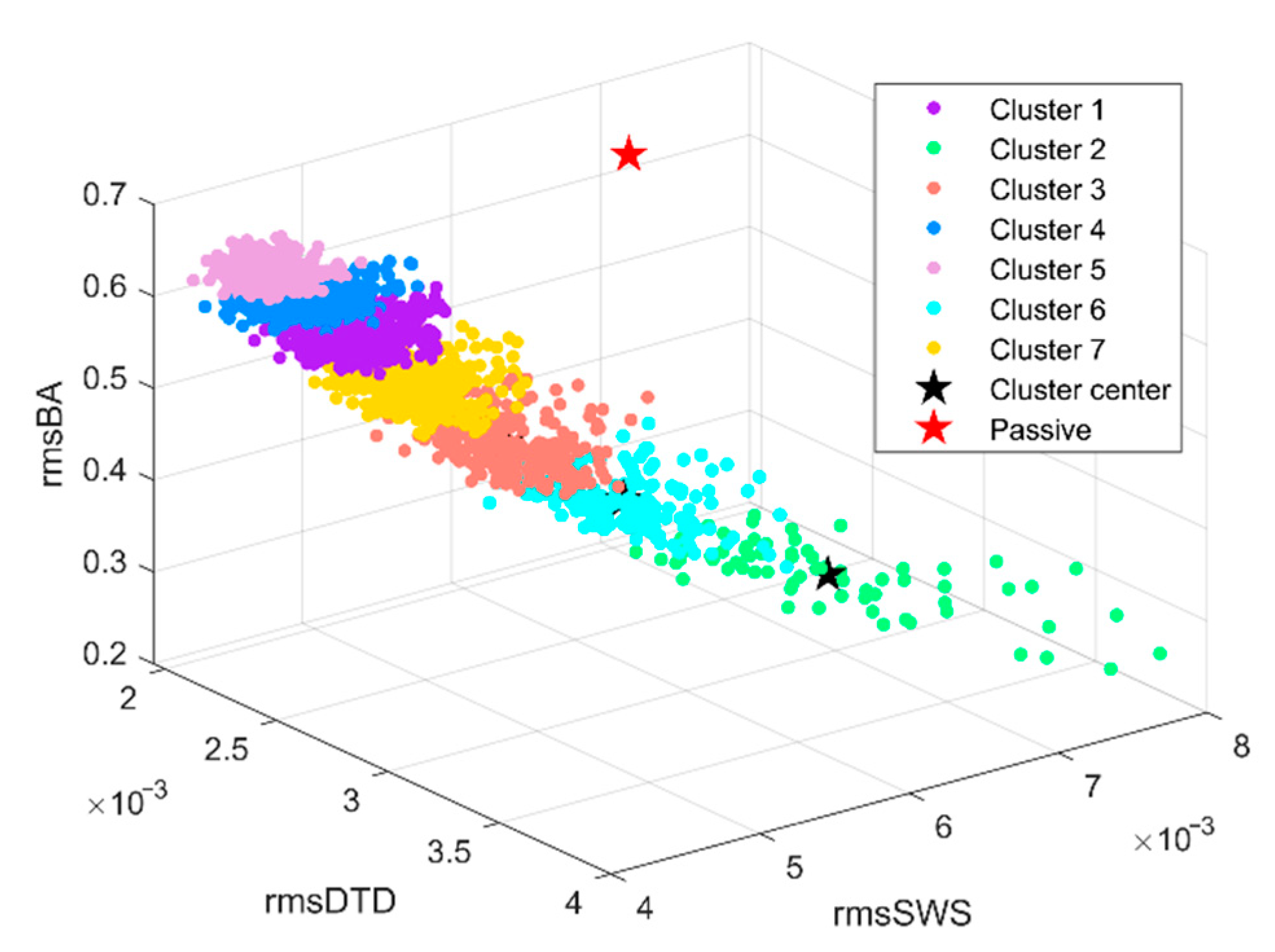
In this paper, the subset of B-class road under 20 m/s (B-20 subset for short) is taken as an example for cluster analysis, which is used to explore the rule information between the weighting coefficients and LQR control effect. The other subsets have the same analysis steps and similar clustering characteristics, which will not be repeated here. A K-means clustering program is written and run to cluster the sample data of the B-20 subset. This subset is divided into seven clusters according to the similarity of the three performance indexes. The clustering results are shown in Figure 10:

As can be seen from Figure 10, the sample data of the B-20 subset are divided into seven clusters, but there is lacking accurate data information to evaluate and analyze the results. Therefore, to accurately describe the clustering effect, the averages of each variable in each cluster are calculated, and all data are processed in ascending order according to the value of the suspension integral performance index $L$. Finally, all the control results are classified into three different suspension requirement modes, which are safety mode, comprehensive mode, and comfort mode. The optimal solutions for the weighting coefficients of each mode are computed. The clustering results are shown in

Table 5. Averages of clustering results of B-20 subset.

Cluster	Number	${\mathit{q}}_1$	${\mathit{q}}_2$	BA/(m·s−2)	SWS/m	DTD/m	dBA	dSWS	dDTD	L	Mode
5	462	100,819	7448	0.6105	0.0046	0.0021	−9.87%	−31.06%	−10.65%	2.4842	safety
4	651	83,348	5899	0.5809	0.0048	0.0021	−13.70%	−28.50%	−7.92%	2.4988
1	497	62,033	5133	0.5474	0.0049	0.0022	−18.60%	−25.71%	−3.50%	2.5219	Comprehensive
7	369	36,170	5662	0.5191	0.0053	0.0022	−27.15%	−29.69%	−3.05%	2.5533
3	276	19,078	5693	0.4596	0.0053	0.0026	−31.65%	−19.80%	15.34%	2.6389	Comfort
6	174	10,904	4452	0.4137	0.0057	0.0029	−38.70%	−14.75%	27.71%	2.7426
2	71	6744	2112	0.3476	0.0064	0.0034	−48.23%	−3.30%	47.01%	2.9548	--

.

Compared with the RMS values of passive suspension, the optimization effect of BA in Cluster 2 is very good, and the optimization rate is as high as 48.23%. However, the DTD deteriorates significantly, and the deterioration rate is as high as 47.01%. Therefore, Cluster 2 should be deleted. For Cluster 5 and Cluster 4, the optimization effect of DTD is the best, which could be classified as safety mode. For Cluster 1 and Cluster 7, the optimization effect of each performance is good, which could be classified as comprehensive mode. For Cluster 3 and Cluster 2, the optimization effect of BA is the most prominent, which is classified as comfort mode.

The clustering results of the remaining 23 kinds of working conditions and the optimal weights of three performance modes can be obtained by the same clustering steps.

Table 6. Optimal solution and simulation results of safety mode under B-class road.

Road Class	Speed	q1	q2	${\mathbf{BA}}_{\mathbf{a}}/(\mathbf{m}·{\mathbf{s}}^{-2})$	${\mathbf{SWS}}_{\mathbf{a}}/\mathbf{m}$	${\mathbf{DTD}}_{\mathbf{a}}/\mathbf{m}$	dBA	dSWS	dDTD	L
B	5	99,211	7328	0.3039	0.0023	0.0010	−10.01%	−30.63%	−10.37%	2.4899
	10	100,830	7493	0.4319	0.0033	0.0015	−9.86%	−31.25%	−10.66%	2.4823
	15	99,191	7433	0.5272	0.0040	0.0018	−9.99%	−30.85%	−10.43%	2.4873
	20	100,819	7448	0.6105	0.0046	0.0021	−9.87%	−31.06%	−10.65%	2.4842
	25	97,983	7389	0.6783	0.0052	0.0023	−10.33%	−30.96%	−10.30%	2.4841
	30	98,991	7473	0.7451	0.0057	0.0025	−10.12%	−31.03%	−10.43%	2.4842

,

Table 7. Optimal solution and simulation results of comprehensive mode under B-class road.

Road Class	Speed	q1	q2	${\mathbf{BA}}_{\mathbf{a}}/(\mathbf{m}·{\mathbf{s}}^{-2})$	${\mathbf{SWS}}_{\mathbf{a}}/\mathbf{m}$	${\mathbf{DTD}}_{\mathbf{a}}/\mathbf{m}$	dBA	dSWS	dDTD	L
B	5	56,998	5298	0.2701	0.0025	0.0011	−19.71%	−25.56%	−2.37%	2.5236
	10	63,974	5208	0.3890	0.0035	0.0015	−18.27%	−26.15%	−4.03%	2.5155
	15	59,460	5158	0.4703	0.0043	0.0019	−19.31%	−25.72%	−2.92%	2.5206
	20	62,033	5133	0.5474	0.0049	0.0022	−18.60%	−25.71%	−3.50%	2.5219
	25	55,367	5247	0.6019	0.0056	0.0025	−20.10%	−25.37%	−1.95%	2.5258
	30	59,849	5224	0.6671	0.0061	0.0027	−19.17%	−25.78%	−3.07%	2.5198

and

Table 8. Optimal solution and simulation results of comfort mode under B-class road.

Road Class	Speed	q1	q2	${\mathbf{BA}}_{\mathbf{a}}/(\mathbf{m}·{\mathbf{s}}^{-2})$	${\mathbf{SWS}}_{\mathbf{a}}/\mathbf{m}$	${\mathbf{DTD}}_{\mathbf{a}}/\mathbf{m}$	dBA	dSWS	dDTD	L
B	5	10,307	4148	0.2018	0.0029	0.0015	−39.85%	−13.98%	29.63%	2.7580
	10	12,278	4882	0.2999	0.0040	0.0020	−36.99%	−16.10%	24.41%	2.7132
	15	10,919	4359	0.3549	0.0049	0.0025	−38.73%	−13.87%	27.82%	2.7522
	20	10,904	4452	0.4137	0.0057	0.0029	−38.70%	−14.75%	27.71%	2.7426
	25	10,588	4329	0.4571	0.0064	0.0033	−39.19%	−14.41%	28.50%	2.7489
	30	10,941	4608	0.5072	0.0069	0.0036	−38.47%	−15.31%	26.97%	2.7319

are the optimal solution and simulation results of safety mode, comprehensive mode, and comfort mode under B-class road, respectively.

Table 9. Optimal solution and simulation results of comfort mode under C-class road.

Road Class	Speed	q1	q2	${\mathbf{BA}}_{\mathbf{a}}/(\mathbf{m}·{\mathbf{s}}^{-2})$	${\mathbf{SWS}}_{\mathbf{a}}/\mathbf{m}$	${\mathbf{DTD}}_{\mathbf{a}}/\mathbf{m}$	dBA	dSWS	dDTD	L
C	5	11,263	4771	0.4188	0.0056	0.0029	−37.89%	−15.67%	26.27%	2.7271
	10	11,334	4830	0.5933	0.0079	0.0041	−37.72%	−15.93%	25.79%	2.7214
	15	9812	4193	0.6983	0.0099	0.0051	−39.91%	−13.53%	30.17%	2.7673
	20	10,551	4378	0.8198	0.0114	0.0059	−39.09%	−14.37%	28.53%	2.7507
	25	11,566	4607	0.9319	0.0126	0.0064	−37.99%	−15.18%	26.23%	2.7307
	30	10,387	4259	0.9970	0.0141	0.0072	−39.64%	−14.18%	28.92%	2.7510

is the optimal solution and simulation results of comfort mode under C-class road. The others are not listed for simplification.

In Table 6, Table 7 and Table 8, the six different rows represent the changes in driving speed. For each row, we performed 2500 simulations with random weighting coefficients. The listed $q_1$ and $q_2$ are the weight’s mean values after mode clustering. Then three performances, BA, SWS, and DTD, are calculated using these $q_1$ and $q_2$. Therefore, the weights would change a lot in different modes, that is to say, the same row’s $q_1$ and $q_2$ are much different among the three tables. However, for the same mode (table), each weight matrix at a different speed may have close values. The analysis on the road changing is similar, comparing Table 8 with Table 9.

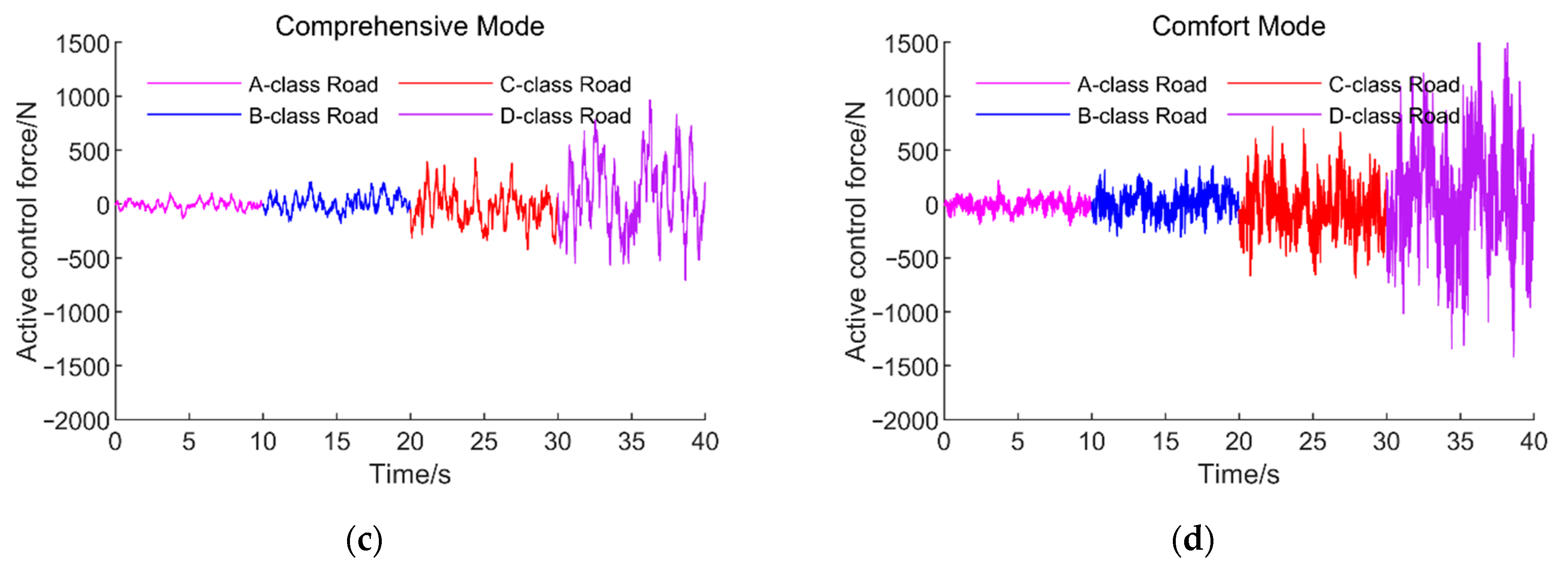
Comparing the data in Table 6, Table 7 and Table 8, different modes have different changing rates of dBA, dSWS, and dDTD. The vehicle speed has less influence on the changing rate. There are diverse control effects of different modes. Comparing the data in Table 7 and Table 8, it can be known that the three changing rates change very little with road conditions and driving velocities. It may prove that our classification with the GKL algorithm could guarantee a stable control effect. Therefore, we could assume that the average values of weight $q_1$ and $q_2$ can be used securely. This assumption also shows good adaptability for the new GKL control. The final values of the optimal weighting coefficients for the three performance modes are shown in

Table 10. The optimal solution of the three performance modes.

Performance Mode	q1	q2	q3
Safety mode	99,971	7434	1
Comprehensive mode	60,829	5154	1
Comfort mode	10,973	4511	1

.

4.3. Simulation Analysis

Using the weighting coefficients list in Table 10, active suspension control with the GKL algorithm is simulated by changing the road conditions and performance modes. The former GA-LQR control is also illustrated for comparison.

4.3.1. Active Control Force

Figure 11 represents the active control force response curves for the four suspension types. In order to qualitatively evaluate the effect of active control, the RMS values of active control force and power consumption are calculated at a vehicle speed of 20 m/s, as shown in

Table 11. RMS values of active control force of each suspension type under different roads.

Suspension Type	$\mathbf{RMS} {\mathit{U}}_{\mathit{a}}/\mathit{N}$
	A-Class Road	B-Class Road	C-Class Road	D-Class Road
GA-LQR control	40.46	75.04	156.83	336.19
Safety mode	39.73	74.19	155.25	326.87
Comprehensive mode	43.62	82.52	170.82	357.94
Comfort mode	62.17	118.33	242.54	516.61

and

Table 12. RMS values of power consumption of each suspension type under different roads.

Suspension Type	RMS Power/W
	A-Class Road	B-Class Road	C-Class Road	D-Class Road
GA-LQR control	28.55	87.16	407.87	1668.42
Safety mode	27.25	83.41	388.06	1614.46
Comprehensive mode	32.58	100.51	460.66	1942.44
Comfort mode	51.10	168.48	745.41	3268.29

.

As can be seen from Table 11 and Table 12, the RMS values of active control force and power consumption in the same mode increase with the road roughness. For the same road input, the active force of safety mode, comprehensive mode, and comfort mode increases in order, which is related to the value of the weighting coefficient of each performance index for different performance modes. With the improvement of comfort requirements, the suspension is required to be soft, so the active control force needs to be larger. The force consumption using GA-LQR is similar to the safety mode but better than the other two modes.

4.3.2. Safety Mode Performances

The optimal solution of weighting coefficients of safety mode is as follows: $q_1=99971$, $q_2=7434$, $q_3=1$. The comparison curves of time domain response of passive suspension and safety mode are shown in Figure 12a–c, and the RMS values of each performance index are shown in Table 12.

As can be seen from

Table 13. RMS values and improvement rate of performance indexes for safety mode.

Road Class	Suspension Type	RMS Values
		BA	SWS	DTD
A	Passive	0.3377	0.0034	0.0011
	GKL (Safety mode)	0.3012	0.0023	0.0010
	Improvement/%	−10.81%	−33.04%	−10.67%
B	Passive	0.6755	0.0068	0.0023
	GKL (Safety mode)	0.6027	0.0043	0.0021
	Improvement/%	−10.79%	−36.70%	−10.56%
C	Passive	1.3526	0.0135	0.0045
	GKL (Safety mode)	1.2016	0.0091	0.0040
	Improvement/%	−11.16%	−33.04%	−10.61%
D	Passive	2.7168	0.0271	0.0093
	GKL (Safety mode)	2.4227	0.0182	0.0083
	Improvement/%	−10.83%	−32.82%	−11.07%

, no matter how the road excitation changes, the safety mode of active suspension designed by the GKL algorithm has similar optimization effects for each performance. This is similar to the discussion in the former clustering evaluation. In the safety mode, the optimization rates of BA, SWS, and DTD are about 10.7%, 33.9%, and 10.7%. In reference [14], the optimization rates of BA, SWS, and DTD for the LQR controller designed based on PSO are around 6.2%, 31%, and 6.5%, respectively. Compared with the active suspension based on PSO-LQR control, there is better optimization in BA, SWS, and DTD. Compared with the active suspension based on GA-LQR control, the improvement effect of DTD is more obvious. This mode can effectively improve the vehicle’s tire grip, which is suitable for aggressive drivers who like to change lanes and overtake.

4.3.3. Comprehensive Mode

The optimal solution of weighting coefficients of comprehensive mode is as follows: $q_1=60829$, $q_2=5154$, $q_3=1$. The comparison curves of time domain response of passive suspension and comprehensive mode are shown in Figure 13a–c, and the RMS values of each performance index are shown in

Table 14. RMS values and improvement rate of performance indexes for comprehensive mode.

Road Class	Suspension Type	RMS Values
		BA	SWS	DTD
A	Passive	0.3377	0.0034	0.0011
	GKL (Comprehensive mode)	0.2714	0.0024	0.0011
	Improvement/%	−19.64%	−29.24%	−3.92%
B	Passive	0.6755	0.0068	0.0023
	GKL (Comprehensive mode)	0.5420	0.0045	0.0022
	Improvement/%	−19.76%	−32.67%	−3.97%
C	Passive	1.3526	0.0135	0.0045
	GKL (Comprehensive mode)	1.0827	0.0096	0.0043
	Improvement/%	−19.96%	−29.24%	−3.92%
D	Passive	2.7168	0.0271	0.0093
	GKL (Comprehensive mode)	2.1897	0.0195	0.0089
	Improvement/%	−19.40%	−28.11%	−4.04%

.

From Table 14, it can be observed that no matter how the road excitation changes, the comprehensive mode of active suspension designed by the GKL algorithm has different degrees of improvement in all performance. In the comprehensive mode, the optimization rates of BA, SWS, and DTD are about 20%, 30%, and 4%, respectively. Compared with the active suspension based on PSO-LQR control [14], the optimization effect of BA is more significant, which greatly improves the comfort of the vehicle. Compared with the passive suspension, this mode effectively improves the comfort and safety of the vehicle. This mode is suitable for the normal type of drivers who pay attention to all performance.

4.3.4. Comfort Mode

The optimal solution of weighting coefficients of comfort mode is as follows: $q_1=10973$, $q_2=4511$, $q_3=1$. The comparison curves of time domain response of passive suspension and comfort mode are shown in Figure 14a–c, and the RMS values of each performance index are shown in

Table 15. RMS values and improvement rate of performance indexes for comfort mode.

Road Class	Suspension Type	RMS Values
		BA	SWS	DTD
A	Passive	0.3377	0.0034	0.0011
	GKL (Comfort mode)	0.2061	0.0027	0.0014
	Improvement/%	−38.98%	−19.62%	25.02%
B	Passive	0.6755	0.0068	0.0023
	GKL (Comfort mode)	0.4000	0.0052	0.0028
	Improvement/%	−40.79%	−23.38%	21.15%
C	Passive	1.3526	0.0135	0.0045
	GKL (Comfort mode)	0.8334	0.0109	0.0056
	Improvement/%	−38.39%	−19.62%	26.37%
D	Passive	2.7168	0.0271	0.0093
	GKL (Comfort mode)	1.6673	0.0224	0.0117
	Improvement/%	−38.63%	−17.31%	25.83%

.

From Table 15, it can be known that no matter how the road excitation changes, the comfort mode of active suspension designed by the GKL algorithm has the most significant improvement in BA. In the comfort mode, the optimization rates of BA and DTD are near 40% and 20%, respectively. Compared with the passive suspension and the active suspension based on GA-LQR, the comfort mode can effectively improve the comfort of the vehicle. This mode is suitable for soft drivers who pay more attention to the body’s vibration response.

5. Conclusions

In this paper, a new GKL method is proposed for suspension control. Based on the traditional LQR control and genetic algorithm, the machine learning idea is introduced to obtain more objective weighting coefficients for different driver types.

The following conclusion can be drawn:

• The proposed GKL algorithm may offer good weight coefficients for the suspension control system’s optimization, and these weights are independent of expert experiences;
• It could be proved that the construct method of weighting space is reasonable. The generated random weights are important to build the machine learning dataset. The dataset could provide 60 thousand sample points for suspension control engineers. Automotive developers can directly select an appropriate weight matrix according to this dataset, which can greatly improve design efficiency by reducing the optimization process of repeated trial and error;
• Through K-means clustering, the active suspension is classified into safety mode, comprehensive mode, and comfort mode, which can adapt to three driving styles: aggressive, normal, and soft. This method offers the LQR control system with two extra solutions, except for the unique value optimized by GA. In future research, we can also use similar ideas combing the support vector machine or deep convolution network with the dataset for parameter optimization;
• The GKL control could improve the suspension performance. The adhesion between the tires and ground increase by 11% in safety mode, and the body acceleration refines by 40% in comfort mode. Moreover, the three performance indexes show good stability for the road input and driving velocity;
• The LQR controller designed based on machine learning ideas has more intuitive design results and richer performance modes. It can meet the different requirements of different drivers for suspension performance or recommend appropriate weighting coefficients according to the different purposes of the vehicle.