Determination of Sugar, pH, and Anthocyanin Contents in Port Wine Grape Berries through Hyperspectral Imaging: An Extensive Comparison of Linear and Non-Linear Predictive Methods
Abstract
1. Introduction
2. Dataset Description
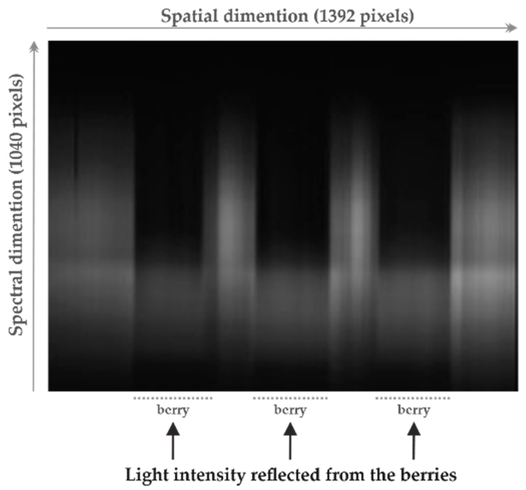
2.1. VIS-NIR Spectral Data Acquisition
2.2. Analytical Determination
3. Linear and Non-Linear Predictive Analytics Comparison Framework: L&NL-PAC
3.1. Preprocessing Approaches
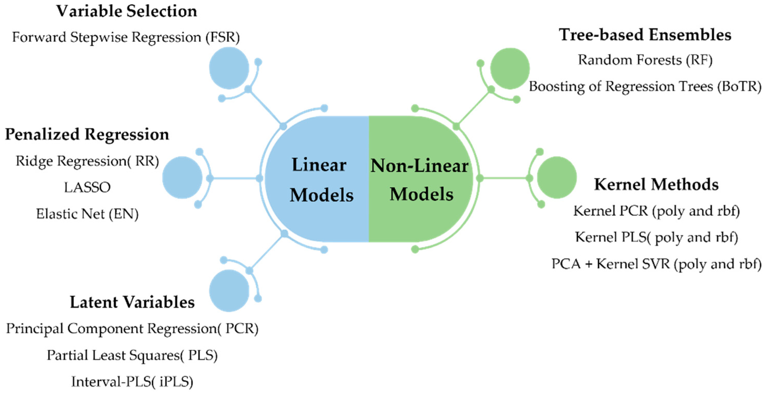
3.2. Predictive Methods
3.2.1. Variable Selection Methods
3.2.2. Penalized Regression Methods
3.2.3. Latent Variable Methods
3.2.4. Tree-Based Ensembles
3.2.5. Kernel Methods
3.3. Model Comparison Methodology
4. Results and Discussion
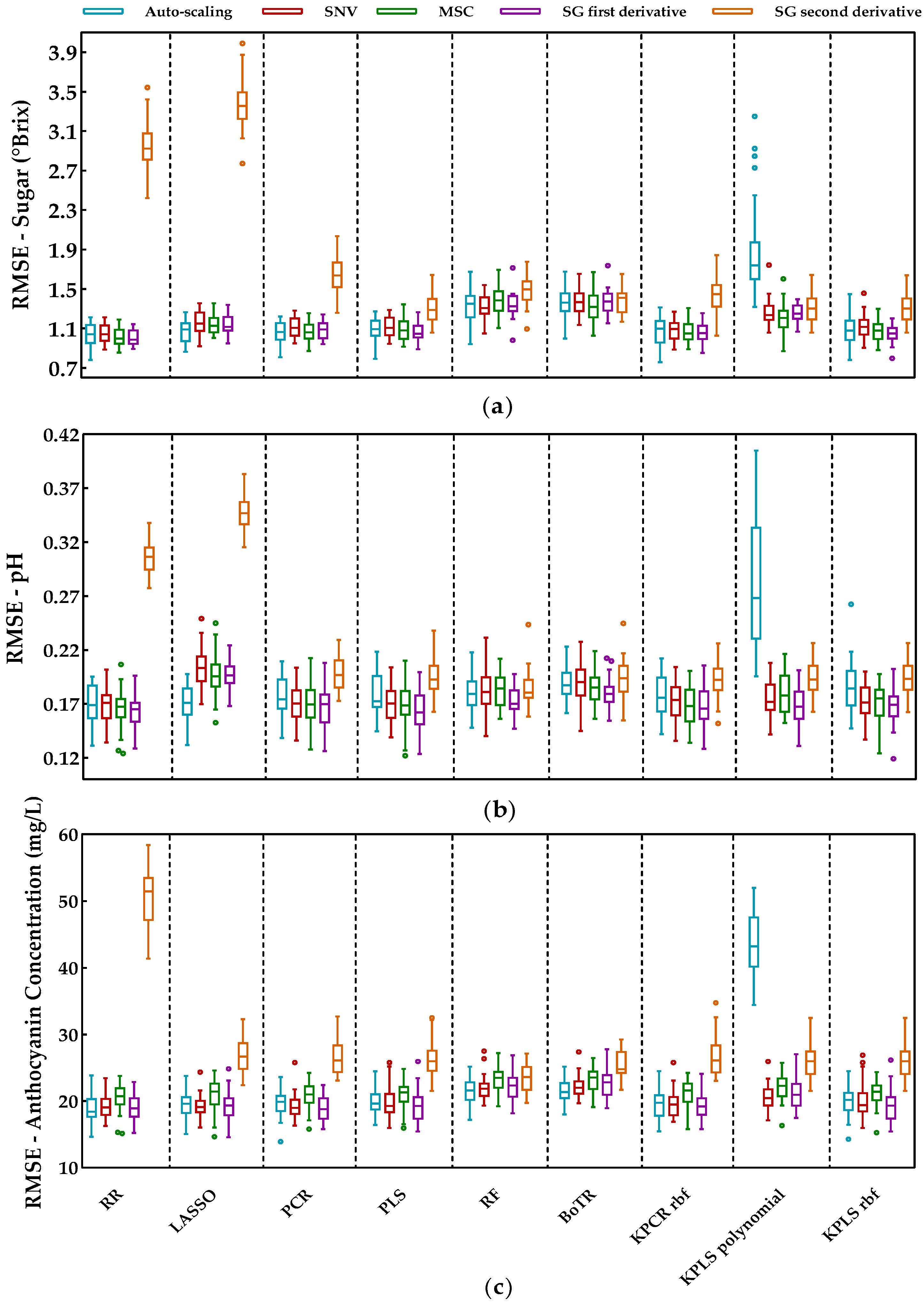
4.1. Preprocessing Evaluation
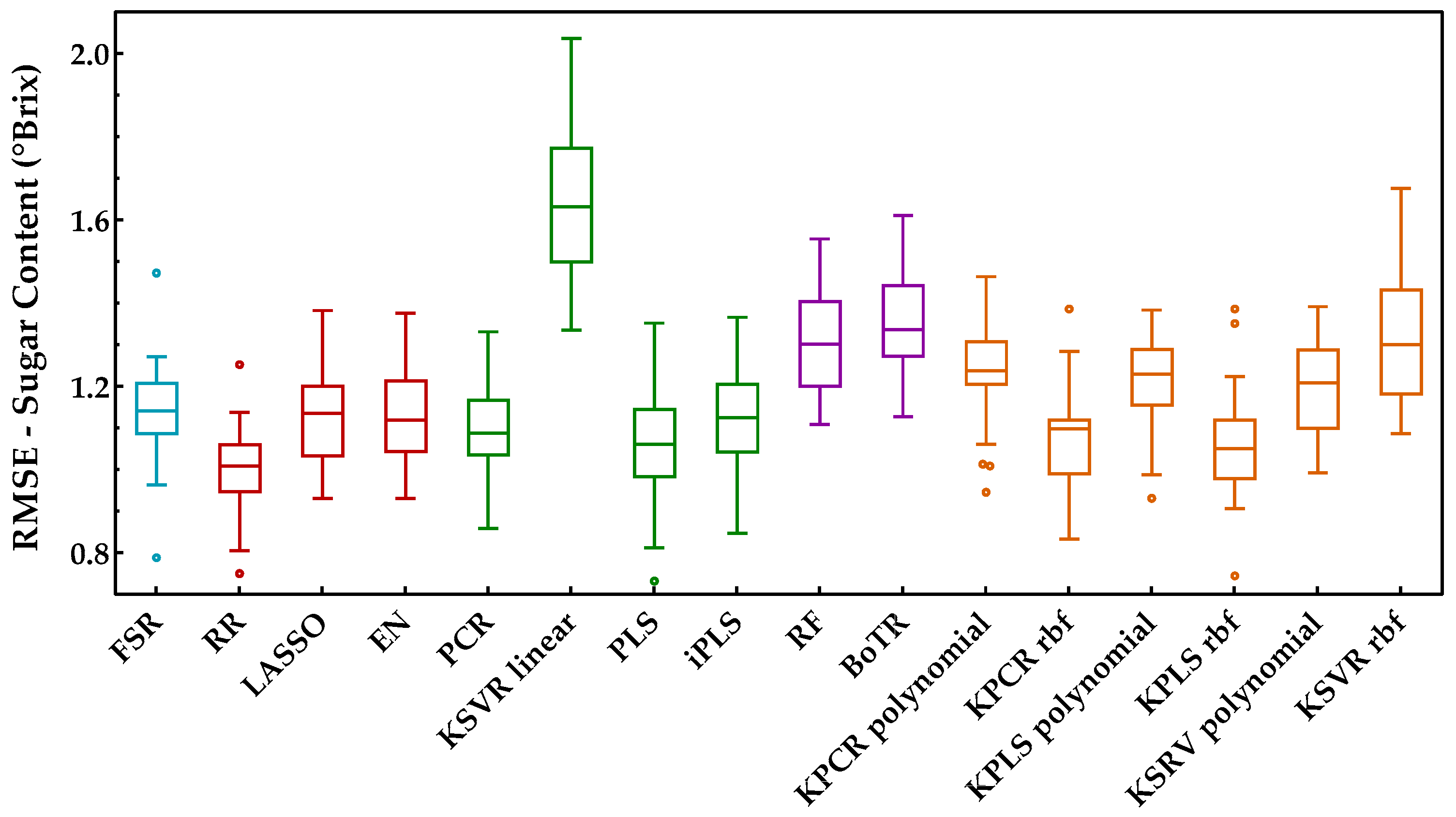
4.2. Sugar Content Analysis
4.3. pH Analysis
4.4. Anthocyanin Concentration Analysis
4.5. Miscellaneous Discussion
5. Conclusions
Author Contributions
Funding
Institutional Review Board Statement
Informed Consent Statement
Acknowledgments
Conflicts of Interest
Appendix A
| Enological Parameters | Mean | SD a | Min b | Max c | Median |
|---|---|---|---|---|---|
| Sugar content (°Brix) | 16.925 | 3.342 | 9.060 | 24.720 | 17.060 |
| pH | 3.552 | 0.346 | 2.850 | 4.230 | 3.580 |
| Anthocyanin concentration (mg·L−1) | 160.278 | 56.860 | 3.894 | 257.819 | 173.841 |
| Enological Parameter | Methods | Auto-Scaling | SNV | MSC | SG 1D | SG 2D |
|---|---|---|---|---|---|---|
| Sugar | RR | 1.039 ± 0.109 | 1.047 ± 0.096 | 1.008 ± 0.092 | 1.004 ± 0.077 | 2.964 ± 0.254 |
| LASSO | 1.072 ± 0.117 | 1.146 ± 0.119 | 1.145 ± 0.105 | 1.138 ± 0.093 | 3.371 ± 0.270 | |
| PCR | 1.058 ± 0.117 | 1.111 ± 0.096 | 1.071 ± 0.099 | 1.089 ± 0.093 | 1.655 ± 0.189 | |
| PLS | 1.098 ± 0.117 | 1.117 ± 0.104 | 1.085 ± 0.106 | 1.061 ± 0.084 | 1.292 ± 0.135 | |
| RF | 1.330 ± 0.161 | 1.315 ± 0.121 | 1.375 ± 0.149 | 1.338 ± 0.128 | 1.486 ± 0.154 | |
| BoTR | 1.358 ± 0.149 | 1.366 ± 0.127 | 1.315 ± 0.148 | 1.370 ± 0.121 | 1.394 ± 0.144 | |
| KPCR rbf | 1.072 ± 0.136 | 1.081 ± 0.098 | 1.058 ± 0.100 | 1.060 ± 0.098 | 1.431 ± 0.184 | |
| KPLS polynomial | 1.897 ± 0.478 | 1.263 ± 0.131 | 1.201 ± 0.152 | 1.259 ± 0.083 | 1.302 ± 0.140 | |
| KPLS rbf | 1.088 ± 0.137 | 1.114 ± 0.120 | 1.070 ± 0.106 | 1.040 ± 0.088 | 13.09 ± 0.148 | |
| pH | RR | 0.170 ± 0.017 | 0.168 ± 0.019 | 0.165 ± 0.018 | 0.163 ± 0.018 | 0.306 ± 0.015 |
| LASSO | 0.172 ± 0.016 | 0.205 ± 0.018 | 0.197 ± 0.019 | 0.196 ± 0.014 | 0.346 ± 0.016 | |
| PCR | 0.176 ± 0.019 | 0.171 ± 0.018 | 0.168 ± 0.019 | 0.168 ± 0.018 | 0.198 ± 0.017 | |
| PLS | 0.178 ± 0.019 | 0.170 ± 0.018 | 0.168 ± 0.020 | 0.165 ± 0.019 | 0.195 ± 0.016 | |
| RF | 0.180 ± 0.016 | 0.182 ± 0.019 | 0.182 ± 0.016 | 0.174 ± 0.013 | 0.184 ± 0.017 | |
| BoTR | 0.189 ± 0.015 | 0.190 ± 0.020 | 0.186 ± 0.017 | 0.180 ± 0.014 | 0.194 ± 0.017 | |
| KPCR rbf | 0.178 ± 0.018 | 0.172 ± 0.017 | 0.168 ± 0.018 | 0.168 ± 0.018 | 0.192 ± 0.016 | |
| KPLS polynomial | 0.283 ± 0.071 | 0.174 ± 0.016 | 0.181 ± 0.020 | 0.168 ± 0.016 | 0.194 ± 0.015 | |
| KPLS rbf | 0.186 ± 0.023 | 0.173 ± 0.017 | 0.170 ± 0.019 | 0.169 ± 0.017 | 0.194 ± 0.016 | |
| Anthocyanins | RR | 18.835 ± 1.925 | 19.090 ± 1.651 | 20.558 ± 2.016 | 18.952 ± 1.965 | 50.597 ± 3.967 |
| LASSO | 19.618 ± 1.807 | 19.249 ± 1.618 | 20.994 ± 2.296 | 19.394 ± 2.190 | 26.770 ± 2.401 | |
| PCR | 19.871 ± 1.885 | 19.170 ± 1.893 | 20.745 ± 2.097 | 18.949 ± 1.673 | 26.528 ± 2.646 | |
| PLS | 19.894 ± 1.804 | 19.759 ± 2.151 | 21.081 ± 1.960 | 19.232 ± 2.285 | 26.121 ± 2.686 | |
| RF | 21.456 ± 1.951 | 22.010 ± 1.819 | 23.262 ± 1.911 | 22.078 ± 2.265 | 23.487 ± 2.151 | |
| BoTR | 21.479 ± 1.837 | 22.010 ± 1.650 | 23.237 ± 1.873 | 22.444 ± 2.142 | 25.500 ± 2.165 | |
| KPCR rbf | 19.514 ± 2.009 | 19.568 ± 1.961 | 21.245 ± 2.013 | 19.459 ± 2.086 | 26.637 ± 2.865 | |
| KPLS polynomial | 49.425 ± 18.671 | 20.722 ± 1.820 | 22.061 ± 2.004 | 21.047 ± 2.260 | 26.048 ± 2.699 | |
| KPLS rbf | 20.047 ± 0.116 | 20.065 ± 0.468 | 21.192 ± 1.920 | 19.445 ± 2.375 | 26.036 ± 2.677 |
| Enological Parameter | Ranking Three Best Methods (1st, 2nd and 3rd Positions) | RMSEP (Mean ± Sd Values) | Rather Important Spectral Regions for the Best Model | Relevant Peaks for the Best Model |
|---|---|---|---|---|
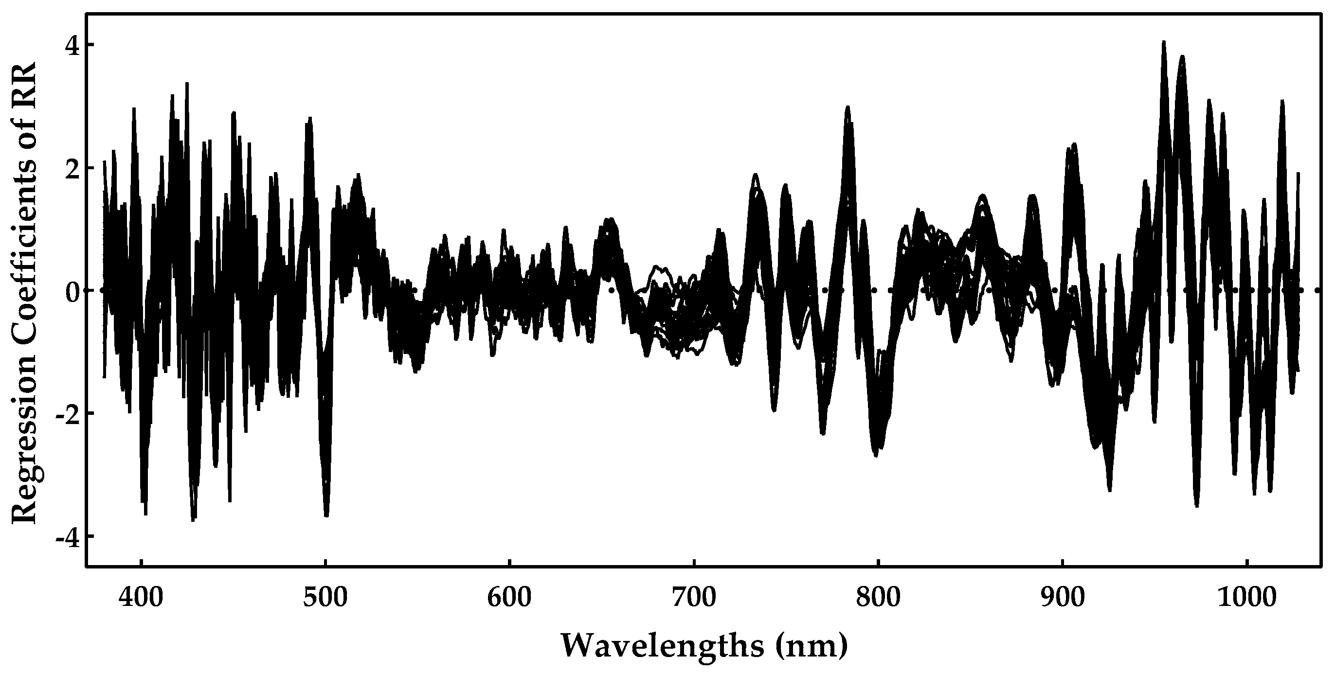
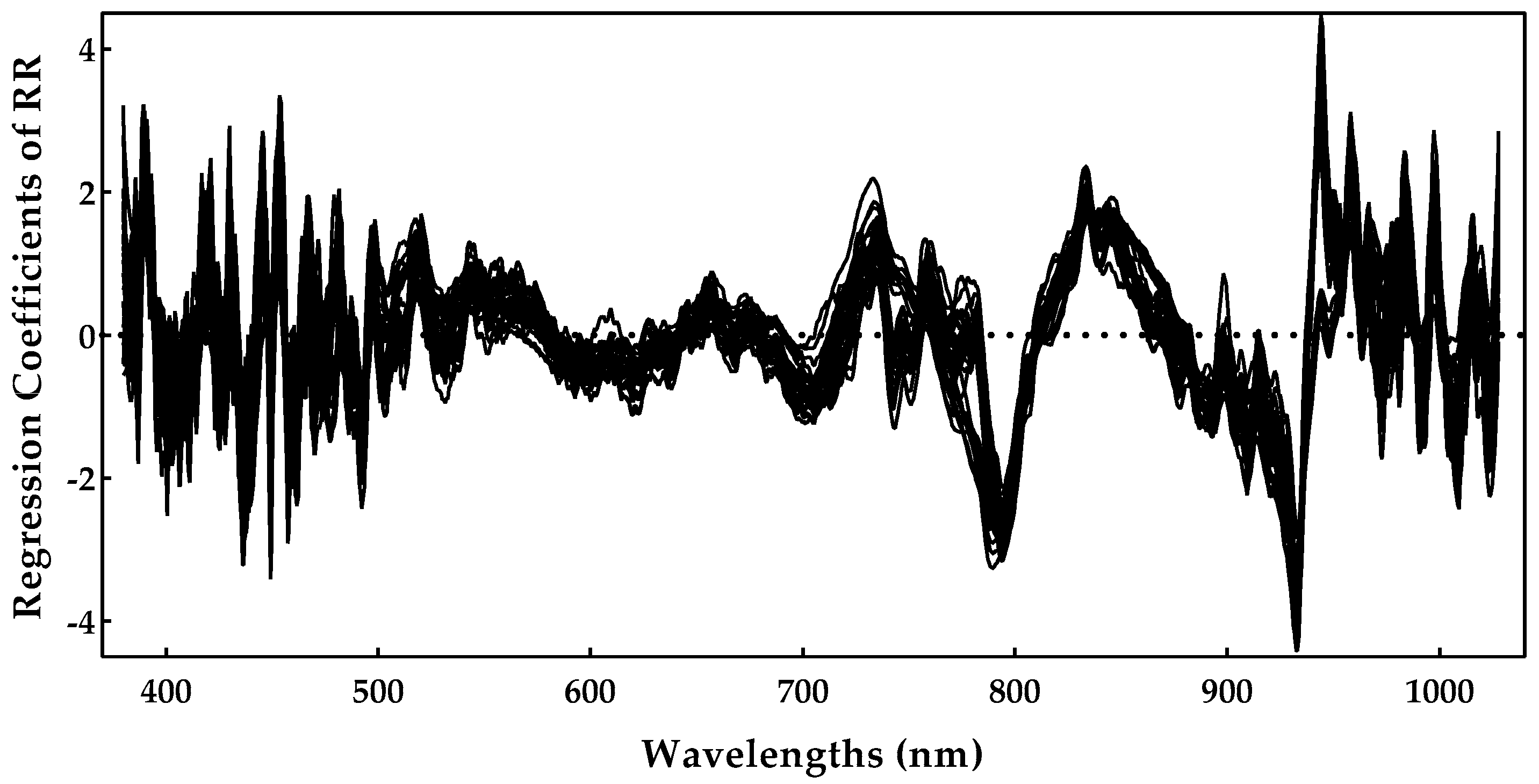
| Sugar content | RR | 0.998 ± 0.102 | 750–800 nm and 900–1000 nm | 770, 920, 960, and 980 nm |
| PLS | 1.055 ± 0.127 | |||
| KPLS rbf | 1.060 ± 0.128 | |||
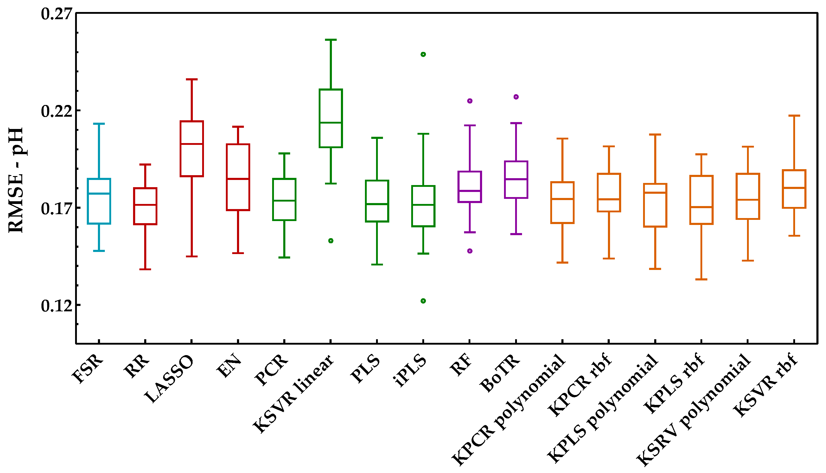
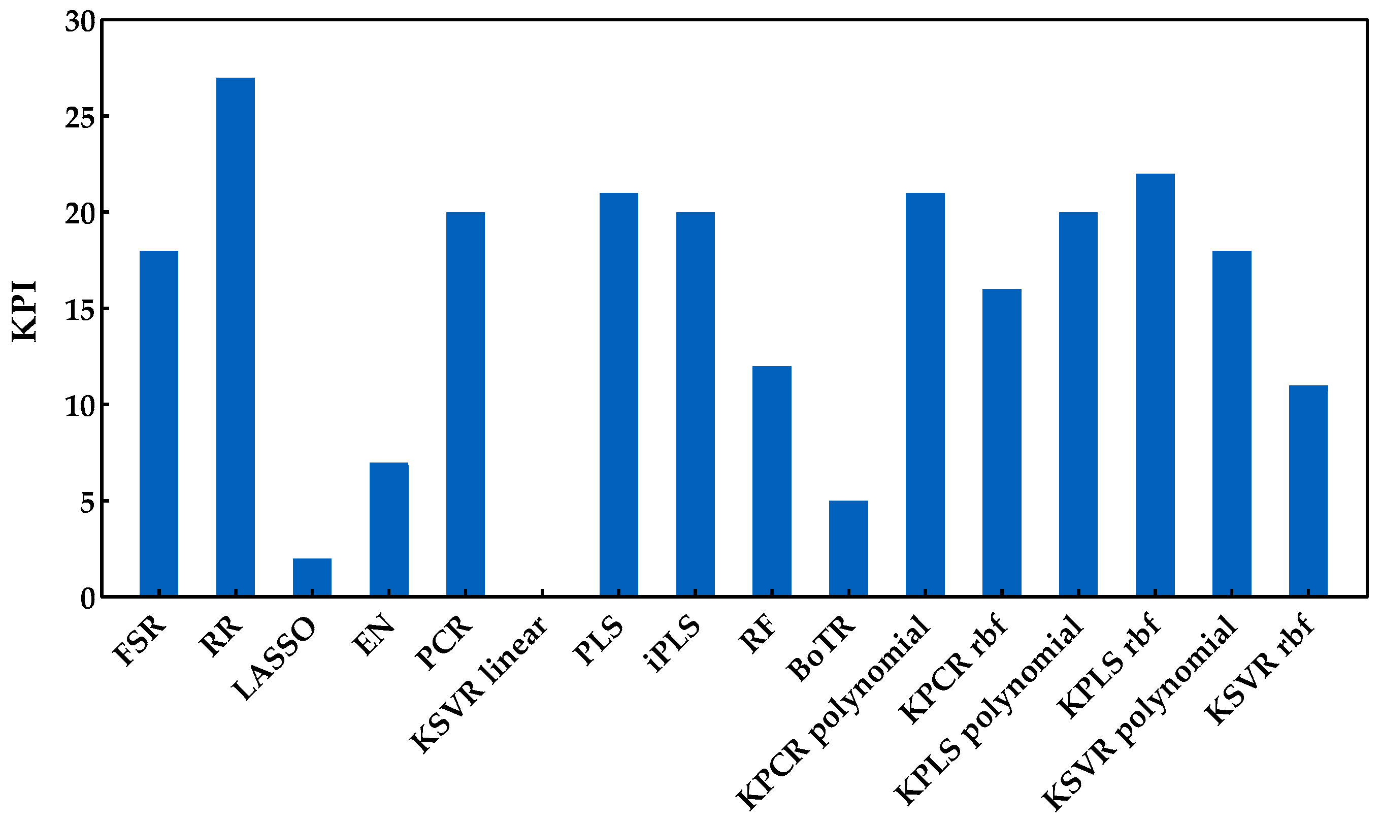
| pH | RR | 0.168 ± 0.014 | 750–950 nm | 790, 840 and 930 nm |
| KPLS rbf | 0.172 ± 0.015 | |||
| PLS/ KPCR polynomial | 0.172 ± 0.015/ 0.175 ± 0.016 | |||
| Anthocyanin concentration | EN | 19.773 ± 2.019 | 400–520 nm and 700–900 nm | 420, 450, 490, 520, 730 and 850 nm |
| PCR | 19.864 ± 2.231 | |||
| RR | 19.961 ± 2.061 |
References
- Chen, Q.; Zhang, C.; Zhao, J.; Ouyang, Q. Recent advances in emerging imaging techniques for non-destructive detection of food quality and safety. TrAC—Trends Anal. Chem. 2013, 52, 261–274. [Google Scholar] [CrossRef]
- Maldonado, A.I.L.; Rodriguez-Fuentes, H.; Contreras, J.A.V. Hyperspectral Imaging in Agriculture, Food and Environment; IntechOpen: London, UK, 2018; ISBN 9781789232905. [Google Scholar]
- Rady, A.M.; Guyer, D.E.; Kirk, W.; Donis-González, I.R. The potential use of visible/near infrared spectroscopy and hyperspectral imaging to predict processing-related constituents of potatoes. J. Food Eng. 2014, 135, 11–25. [Google Scholar] [CrossRef]
- Sun, D.W. Hyperspectral Imaging for Food Quality Analysis and Control; Elsevier: Amsterdam, The Netherlands, 2010; ISBN 9780123747532. [Google Scholar]
- Huang, H.; Liu, L.; Ngadi, M.O. Recent developments in hyperspectral imaging for assessment of food quality and safety. Sensors 2014, 14, 7248–7276. [Google Scholar] [CrossRef]
- Fernandes, A.; Gomes, V.; Melo-Pinto, P. A Review of the Application to Emergent Subfields in Viticulture of Local Reflectance and Interactance Spectroscopy Combined with Soft Computing and Multivariate Analysis BT. In Soft Computing for Sustainability Science; Cruz Corona, C., Ed.; Springer International Publishing: Cham, Switzerland, 2018; pp. 87–115. ISBN 978-3-319-62359-7. [Google Scholar]
- Gomes, V.M.; Fernandes, A.M.; Faia, A.; Melo-Pinto, P. Comparison of different approaches for the prediction of sugar content in new vintages of whole Port wine grape berries using hyperspectral imaging. Comput. Electron. Agric. 2017, 140, 244–254. [Google Scholar] [CrossRef]
- Nogales-Bueno, J.; Hernández-Hierro, J.M.; Rodríguez-Pulido, F.J.; Heredia, F.J. Determination of technological maturity of grapes and total phenolic compounds of grape skins in red and white cultivars during ripening by near infrared hyperspectral image: A preliminary approach. Food Chem. 2014, 152, 586–591. [Google Scholar] [CrossRef] [PubMed]
- Chen, S.; Zhang, F.; Ning, J.; Liu, X.; Zhang, Z.; Yang, S. Predicting the anthocyanin content of wine grapes by NIR hyperspectral imaging. Food Chem. 2015, 172, 788–793. [Google Scholar] [CrossRef] [PubMed]
- dos Santos Costa, D.; Oliveros Mesa, N.F.; Santos Freire, M.; Pereira Ramos, R.; Teruel Mederos, B.J. Development of predictive models for quality and maturation stage attributes of wine grapes using vis-nir reflectance spectroscopy. Postharvest Biol. Technol. 2019, 150, 166–178. [Google Scholar] [CrossRef]
- Fadock, M.; Brown, R.B.; Reynolds, A.G. Visible-Near Infrared Reflectance Spectroscopy for Nondestructive Analysis of Red Wine Grapes. Am. J. Enol. Vitic. 2016, 67, 38–46. [Google Scholar] [CrossRef]
- Silva, R.; Gomes, V.; Mendes-Faia, A.; Melo-Pinto, P. Using support vector regression and hyperspectral imaging for the prediction of oenological parameters on different vintages and varieties ofwine grape berries. Remote Sens. 2018, 10, 312. [Google Scholar] [CrossRef]
- Fernandes, A.M.; Franco, C.; Mendes-Ferreira, A.; Mendes-Faia, A.; da Costa, P.L.; Melo-Pinto, P. Brix, pH and anthocyanin content determination in whole Port wine grape berries by hyperspectral imaging and neural networks. Comput. Electron. Agric. 2015, 115, 88–96. [Google Scholar] [CrossRef]
- Gomes, V.; Fernandes, A.; Martins-Lopes, P.; Pereira, L.; Mendes Faia, A.; Melo-Pinto, P. Characterization of neural network generalization in the determination of pH and anthocyanin content of wine grape in new vintages and varieties. Food Chem. 2017, 218, 40–46. [Google Scholar] [CrossRef]
- Arana, I.; Jarén, C.; Arazuri, S. Maturity, variety and origin determination in white grapes (Vitis vinifera L.) using near infrared reflectance technology. J. Near Infrared Spectrosc. 2005, 13, 349–357. [Google Scholar] [CrossRef]
- González-Caballero, V.; Pérez-Marín, D.; López, M.-I.; Sánchez, M.-T. Optimization of NIR Spectral Data Management for Quality Control of Grape Bunches during On-Vine Ripening. Sensors 2011, 11, 6109–6124. [Google Scholar] [CrossRef]
- Janik, L.J.; Cozzolino, D.; Dambergs, R.; Cynkar, W.; Gishen, M. The prediction of total anthocyanin concentration in red-grape homogenates using visible-near-infrared spectroscopy and artificial neural networks. Anal. Chim. Acta 2007, 594, 107–118. [Google Scholar] [CrossRef]
- Le Moigne, M.; Dufour, E.; Bertrand, D.; Maury, C.; Seraphin, D.; Jourjon, F. Front face fluorescence spectroscopy and visible spectroscopy coupled with chemometrics have the potential to characterise ripening of Cabernet Franc grapes. Anal. Chim. Acta 2008, 621, 8–18. [Google Scholar] [CrossRef] [PubMed]
- Organisation International de la Vigne e du Vin. Recueil des Méthodes Internationales D’analyse des vins et des Mouts. OIV 2009. Available online: https://www.franceagrimer.fr/content/download/29260/259660/file/recueil_methodes_d_analyse_2009_vol1_fr.pdf (accessed on 21 September 2021).
- Riberéau-Gayon, P.; Stonestreet, E. La dosage des anthocyanes dans les vins rouge. Bull. Société Chim. 1965, 9, 2649. [Google Scholar]
- Purwanto, Y.A.; Sari, H.P.; Budiastra, I.W. Effects of preprocessing techniques in developing a calibration model for soluble solid and acidity in “Gedong Gincu” mango using NIR spectroscopy. Int. J. Eng. Technol. 2015, 7, 1921–1927. [Google Scholar]
- Sarkar, S.; Basak, J.K.; Moon, B.E.; Kim, H.T. A comparative study of PLSR and SVM-R with various preprocessing techniques for the quantitative determination of soluble solids content of hardy kiwi fruit by a portable Vis/NIR spectrometer. Foods 2020, 9, 1078. [Google Scholar] [CrossRef] [PubMed]
- Pahlawan, M.F.R.; Wati, R.K.; Masithoh, R.E. Development of a low-cost modular VIS/NIR spectroscopy for predicting soluble solid content of banana. In Proceedings of the IOP Conference Series: Earth and Environmental Science; IOP Publishing Ltd.: Bristol, UK, 2021; Volume 644, p. 012047. [Google Scholar]
- Zhang, Y.; Guo, W. Moisture content detection of maize seed based on visible/near-infrared and near-infrared hyperspectral imaging technology. Int. J. Food Sci. Technol. 2020, 55, 631–640. [Google Scholar] [CrossRef]
- Yu, H.; Guo, L.; Kharbach, M.; Han, W. Multi-way analysis coupled with near-infrared spectroscopy in food industry: Models and applications. Foods 2021, 10, 802. [Google Scholar] [CrossRef]
- Sun, D.W. Infrared Spectroscopy for Food Quality Analysis and Control; Academic Press, Elsevier: San Diego, CA, USA, 2009; ISBN 9780123741363. [Google Scholar]
- Rinnan, Å.; van den Berg, F.; Engelsen, S.B. Review of the most common pre-processing techniques for near-infrared spectra. TrAC—Trends Anal. Chem. 2009, 28, 1201–1222. [Google Scholar] [CrossRef]
- Barnes, R.J.; Dhanoa, M.S.; Lister, S.J. Standard normal variate transformation and de-trending of near-infrared diffuse reflectance spectra. Appl. Spectrosc. 1989, 43, 772–777. [Google Scholar] [CrossRef]
- Gautam, R.; Vanga, S.; Ariese, F.; Umapathy, S. Review of multidimensional data processing approaches for Raman and infrared spectroscopy. EPJ Tech. Instrum. 2015, 2, 8. [Google Scholar] [CrossRef]
- Zeaiter, M.; Rutledge, D. Preprocessing Methods. In Comprehensive Chemometrics: Chemical and Biochemical Data Analysis; Brown, S.D., Tauler, R., Walczak, B., Eds.; Elsevier: Amsterdam, The Netherlands, 2009; pp. 121–231. ISBN 978-0-444-52701-1. [Google Scholar]
- Sun, T.; Xu, W.; Wang, X.; Liu, M. Improvement of Soluble Solids Content Prediction in Navel Oranges by Vis/NIR Semi-Transmission Spectra and UVE-GA-LSSVM. In Knowledge Engineering and Management; Springer: Berlin/Heidelberg, Germany, 2014; pp. 363–372. [Google Scholar]
- Jiao, Y.; Li, Z.; Chen, X.; Fei, S. Preprocessing methods for near-infrared spectrum calibration. J. Chemom. 2020, 34, e3306. [Google Scholar] [CrossRef]
- Bi, Y.; Yuan, K.; Xiao, W.; Wu, J.; Shi, C.; Xia, J.; Chu, G.; Zhang, G.; Zhou, G. A local pre-processing method for near-infrared spectra, combined with spectral segmentation and standard normal variate transformation. Anal. Chim. Acta 2016, 909, 30–40. [Google Scholar] [CrossRef]
- Sadeghi, M.; Behnia, F.; Amiri, R. Window Selection of the Savitzky-Golay Filters for Signal Recovery from Noisy Measurements. IEEE Trans. Instrum. Meas. 2020, 69, 5418–5427. [Google Scholar] [CrossRef]
- Rendall, R.; Reis, M.S. Which regression method to use? Making informed decisions in “data-rich/knowledge poor” scenarios—The Predictive Analytics Comparison framework (PAC). Chemom. Intell. Lab. Syst. 2018, 181, 52–63. [Google Scholar] [CrossRef]
- Cao, D.S.; Liang, Y.Z.; Xu, Q.S.; Hu, Q.N.; Zhang, L.X.; Fu, G.H. Exploring nonlinear relationships in chemical data using kernel-based methods. Chemom. Intell. Lab. Syst. 2011, 107, 106–115. [Google Scholar] [CrossRef]
- Cristianini, N.; Shawe-Taylor, J. An Introduction to Support Vector Machines and Other Kernel-based Learning Methods; Cambridge University Press: Cambridge, UK, 2000. [Google Scholar]
- Müller, K.R.; Mika, S.; Rätsch, G.; Tsuda, K.; Schölkopf, B. An introduction to kernel-based learning algorithms. IEEE Trans. Neural Netw. 2001, 12, 181–201. [Google Scholar] [CrossRef] [PubMed]
- Williams, P.C. Implementation of near-infrared technology. In Near-Infrared Technology in the Agricultural and Food Industries; American Association of Cereal Chemistry: St. Paul, MN, USA, 2001. [Google Scholar]
- Piazzolla, F.; Amodio, M.L.; Colelli, G. Spectra evolution over on-vine holding of italia table grapes: Prediction of maturity and discrimination for harvest times using a Vis-NIR hyperspectral device. J. Agric. Eng. 2017, 48, 109–116. [Google Scholar] [CrossRef][Green Version]
- Cao, F.; Wu, D.; He, Y. Soluble solids content and pH prediction and varieties discrimination of grapes based on visible–near infrared spectroscopy. Comput. Electron. Agric. 2010, 71, S15–S18. [Google Scholar] [CrossRef]


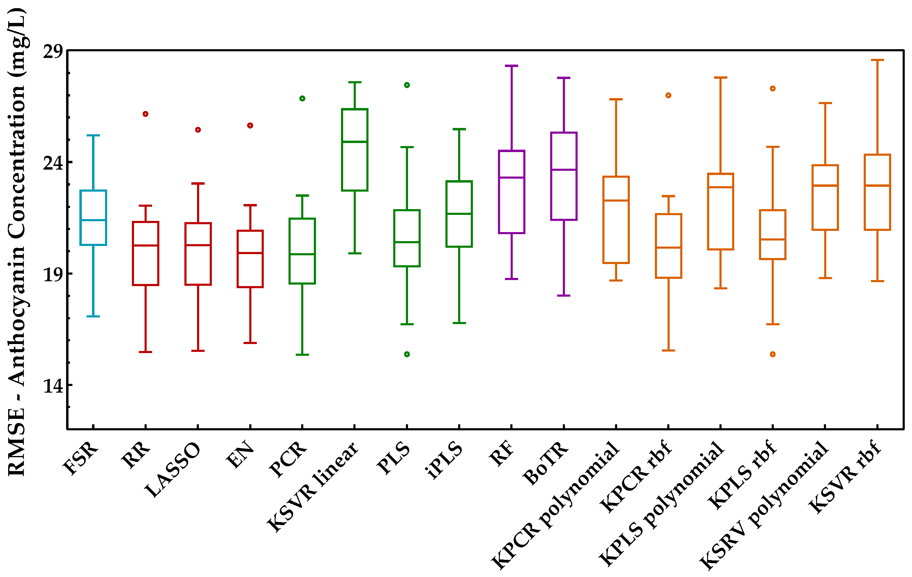
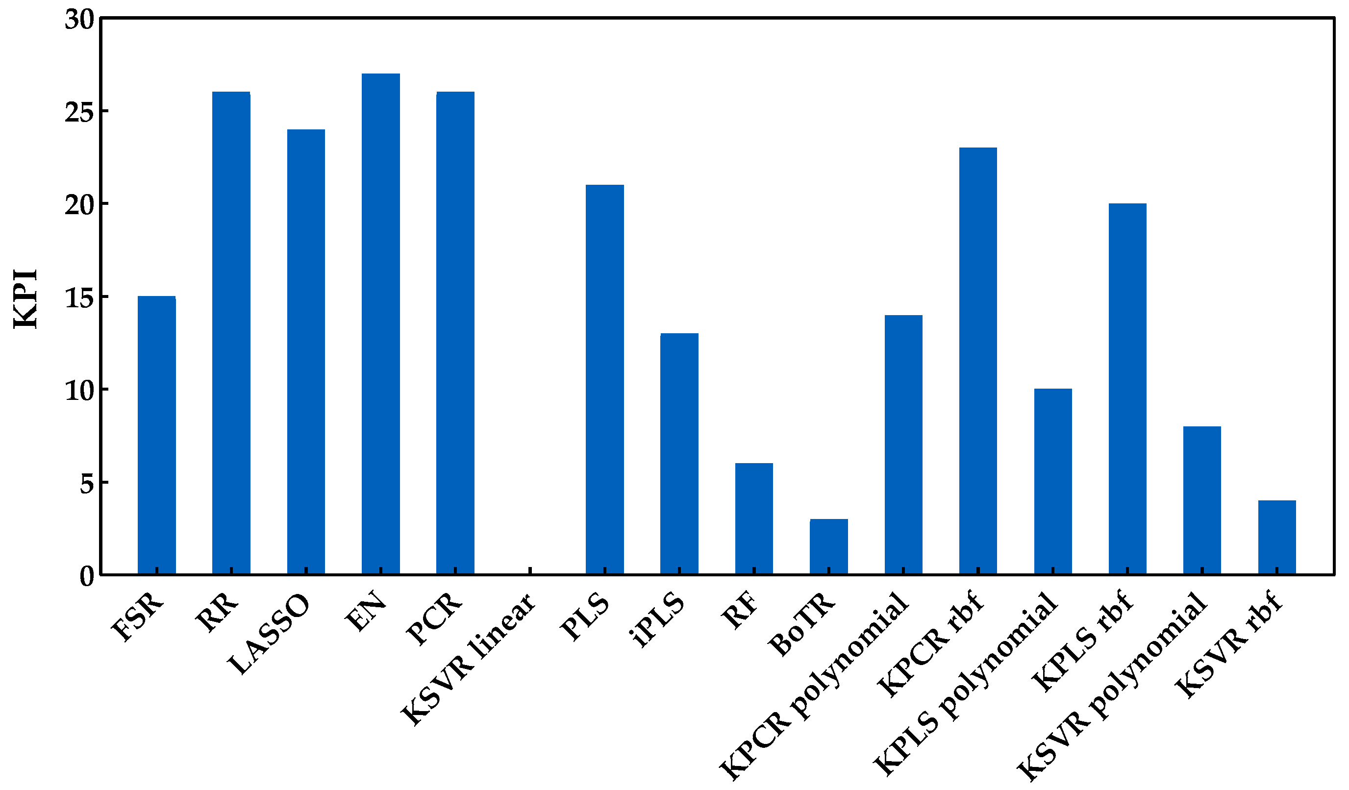
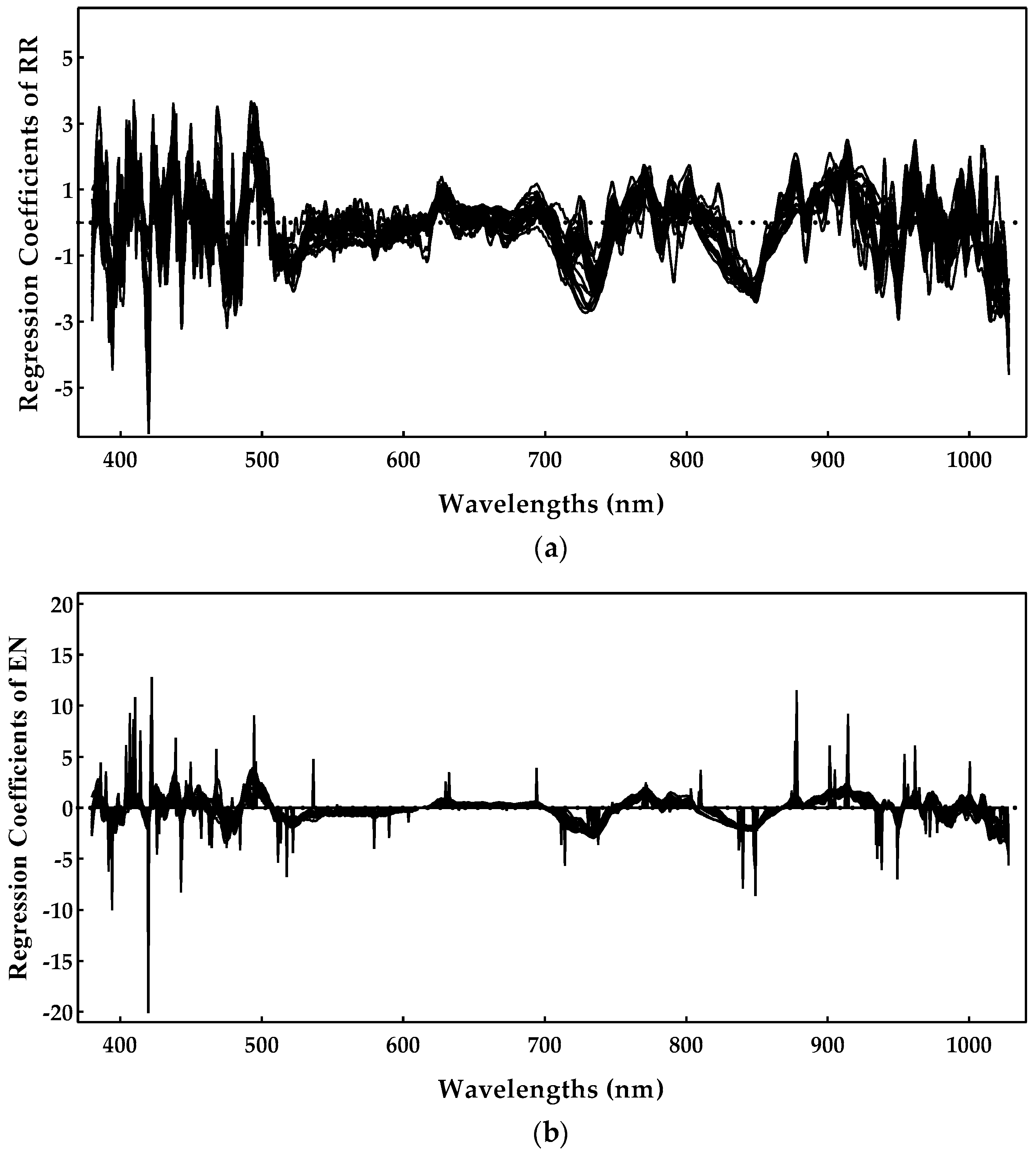
| Ref. | Methods | Preprocessing | RMSE | ||
|---|---|---|---|---|---|
| Sugar (°Brix) | pH | Anthocyanin | |||
| [7] a | PLS | Normalization | 0.940–1.340 | - | - |
| ANN | 0.960–1.360 | ||||
| [8] | MPLS 1 | Raw | 1.370 | - | - |
| MSC | 1.610 | 0.180 | |||
| SNV | 1.890 | - | |||
| [9] | PLS | Raw | - | - | 0.015 mg·g−1 |
| SG | 0.013 mg·g−1 | ||||
| SNV | 0.013 mg·g−1 | ||||
| MSC | 0.022 mg·g−1 | ||||
| 1st derivative | 0.041 mg·g−1 | ||||
| 2nd derivative | 0.028 mg·g−1 | ||||
| PLS + SVM 2 | SG | - | - | 0.005 mg·g−1 | |
| [10] | PLS | MSC | 1.150 | - | - |
| SNV | 1.380 | 13.560 cg·kg−1 | |||
| PCR 3 | MSC | 1.630 | - | - | |
| SNV | 1.410 | 13.660 cg·kg−1 | |||
| MLR 4 | SNV | 1.530 | - | 17.980 cg·kg−1 | |
| [11] | PLS | Raw | 0.650 | 0.050 | - |
| Normalization | 0.870 | 0.050 | 74.670 mg·L−1 | ||
| SG | 0.650 | 0.050 | - | ||
| SNV | 1.830 | 0.080 | - | ||
| [13] | ANN | Normalization | 0.950 | 0.180 | 14.000 mg·L−1 |
| [14] a | ANN | Normalization | - | 0.170–0.190 | 22.100–51.300 mg·L−1 |
| [12] a | SVM 2 | Normalization | 0.800–1.410 | 0.140–0.190 | 11.750–18.020 mg·L−1 |
| [15] b | PLS | SG (1st and 2nd derivative) | 1.270–2.160 | - | - |
| [16] | MPLS | 1st derivative | - | 0.170 | - |
| 2nd derivative | 1.690 | - | |||
| LOCAL | 1st derivative | - | 0.150 | ||
| 2nd derivative | 1.320 | - | |||
| [17] | PLS | SG | - | - | 0.160 mg·g−1 |
| PLS-ANN | 0.18 mg·g−1 | ||||
| [18] b | PLS | - | - | - | 1.510 mg·g−1 |
| Method | Hyperparameter | Range Values |
|---|---|---|
| FSR | penter | 0.05 |
| prem | 0.1 | |
| RR | α | 0 |
| γ | 0.002; 0.02; 0.2; 2; 20 | |
| LASSO | α | 1 |
| γ | 0.001; 0.01; 0.1; 1; 10 | |
| EN | α | 0.001; 0.01; 0.1; 1 |
| γ | 0.002; 0.02; 0.2; 2; 20 | |
| SVR Linear | aPCR | [1:min(20, n, p)] |
| ε | 0.005; 0.01; 0.05; 0.1 | |
| PCR | aPCR | [1:min(20, n, p)] |
| PLS | aPLS | [1:min(20, n, p)] |
| iPLS | aiPLS | [1:min(20, n, p)] |
| RF | TRF | 50; 100; 500; 1000; 5000 |
| BoRT | TBT | 50; 100; 500; 1000; 5000 |
| KPCR | aPCR | [1:30] |
| Polynomial: p | [2:10] | |
| Rbf: σ | 0.1; 1; 10; 50; 100; 300; 1000 | |
| KPLS | aPCR | [1:30] |
| Polynomial: p | [2:10] | |
| Rbf: σ | 0.1; 1; 10; 50; 100; 300; 1000 | |
| KSVR | aPCR | [1:20] |
| ε | 0.005; 0.01; 0.05; 0.1 | |
| Polynomial: p | [2:6] | |
| Rbf: σ | 0.1; 1; 10; 50; 100; 300; 1000 |
| Method | RPD | RER | ||
|---|---|---|---|---|
| Mean | 95% CI | Mean | 95% CI | |
| FSR | 2.916 | (2.781; 3.051) | 12.130 | (11.590; 12.671) |
| RR | 3.321 | (3.161; 3.482) | 13.828 | (13.144; 14.512) |
| LASSO | 2.940 | (2.808; 3.073) | 12.248 | (11.660; 12.836) |
| EN | 2.936 | (2.809; 3.063) | 12.230 | (11.662; 12.798) |
| PCR | 3.038 | (2.891; 3.185) | 12.660 | (11.999; 13.321) |
| KSVR linear | 2.008 | (1.943; 2.074) | 8.3706 | (8.049; 8.692) |
| PLS | 3.160 | (2.978; 3.342) | 13.167 | (12.374; 13.959) |
| iPLS | 2.946 | (2.799; 3.093) | 12.251 | (11.678; 12.823) |
| RF | 2.511 | (2.409; 2.613) | 10.464 | (9.989; 10.939) |
| BoTR | 2.451 | (2.357; 2.546) | 10.214 | (9.778; 10.651) |
| KPCR polynomial | 2.698 | (2.574; 2.823) | 11.231 | (10.716; 11.746) |
| KPCR rbf | 3.083 | (2.943; 3.222) | 12.840 | (12.231; 13.449) |
| KPLS polynomial | 2.728 | (2.608; 2.849) | 11.356 | (10.858; 11.854) |
| KPLS rbf | 3.139 | (2.970; 3.307) | 13.076 | (12.341; 13.811) |
| KSVR polynomial | 2.756 | (2.644; 2.869) | 11.480 | (10.987; 11.972) |
| KSVR rbf | 2.521 | (2.417; 2.624) | 10.502 | (10.029; 10.975) |
| Method | RPD | RER | ||
|---|---|---|---|---|
| Mean | 95% CI | Mean | 95% CI | |
| FSR | 2.012 | (1.942; 2.082) | 7.407 | (7.117; 7.696) |
| RR | 2.085 | (2.015; 2.155) | 7.670 | (7.397; 7.944) |
| LASSO | 1.766 | (1.697; 1.835) | 6.501 | (6.223; 6.779) |
| EN | 1.916 | (1.847; 1.985) | 7.051 | (6.775; 7.327) |
| PCR | 2.029 | (1.965; 2.094) | 7.463 | (7.216; 7.711) |
| KSVR linear | 1.654 | (1.587; 1.720) | 6.088 | (5.819; 6.355) |
| PLS | 2.052 | (1.981; 2.124) | 7.548 | (7.274; 7.822) |
| iPLS | 2.055 | (1.975; 2.134) | 7.563 | (7.248; 7.878) |
| RF | 1.958 | (1.890; 2.027) | 7.206 | (6.935; 7.476) |
| BoTR | 1.898 | (1.836; 1.960) | 6.982 | (6.737; 7.228) |
| KPCR polynomial | 2.047 | (1.984; 2.110) | 7.529 | (7.279; 7.779) |
| KPCR rbf | 1.999 | (1.934; 2.059) | 7.352 | (7.116; 7.588) |
| KPLS polynomial | 2.037 | (1.968; 2.106) | 7.493 | (7.226; 7.760) |
| KPLS rbf | 2.054 | (1.986; 2.123) | 7.556 | (7.292; 7.819) |
| KSVR polynomial | 2.012 | (1.945; 2.078) | 7.399 | (7.145; 7.653) |
| KSVR rbf | 1.952 | (1.896; 2.008) | 7.186 | (6.941; 7.432) |
| Method | RPD | RER | ||
|---|---|---|---|---|
| Mean | 95% CI | Mean | 95% CI | |
| FSR | 2.747 | (2.617; 2.877) | 10.950 | (10.451; 11.450) |
| RR | 2.921 | (2.784; 3.059) | 11.654 | (11.108; 12.200) |
| LASSO | 2.915 | (2.780; 3.052) | 11.635 | (11.071; 12.199) |
| EN | 2.947 | (2.814; 3.081) | 11.762 | (11.214; 12.311) |
| PCR | 2.939 | (2.799; 3.079) | 11.726 | (11.163; 12.289) |
| KSVR linear | 2.393 | (2.278; 2.509) | 9.536 | (9.098; 9.974) |
| PLS | 2.838 | (2.698; 2.978) | 11.321 | (10.773; 11.869) |
| iPLS | 2.701 | (2.561; 2.840) | 10.755 | (10.259; 11.250) |
| RF | 2.548 | (2.417; 2.679) | 10.146 | (9.670; 10.621) |
| BoTR | 2.501 | (2.378; 2.624) | 9.965 | (9.491; 10.438) |
| KPCR polynomial | 2.687 | (2.555; 2.819) | 10.724 | (10.177; 11.272) |
| KPCR rbf | 2.893 | (2.753; 3.034) | 11.546 | (10.979; 12.114) |
| KPLS polynomial | 2.640 | (2.510; 2.770) | 10.626 | (10.022; 11.030) |
| KPLS rbf | 2.835 | (2.698; 2.970) | 11.312 | (10.759; 11.865) |
| KSVR polynomial | 2.586 | (2.467; 2.705) | 10.310 | (9.843; 10.777) |
| KSVR rbf | 2.540 | (2.420; 2.660) | 10.129 | (9.654; 10.604) |
Publisher’s Note: MDPI stays neutral with regard to jurisdictional claims in published maps and institutional affiliations. |
© 2021 by the authors. Licensee MDPI, Basel, Switzerland. This article is an open access article distributed under the terms and conditions of the Creative Commons Attribution (CC BY) license (https://creativecommons.org/licenses/by/4.0/).
Share and Cite
Gomes, V.; Rendall, R.; Reis, M.S.; Mendes-Ferreira, A.; Melo-Pinto, P. Determination of Sugar, pH, and Anthocyanin Contents in Port Wine Grape Berries through Hyperspectral Imaging: An Extensive Comparison of Linear and Non-Linear Predictive Methods. Appl. Sci. 2021, 11, 10319. https://doi.org/10.3390/app112110319
Gomes V, Rendall R, Reis MS, Mendes-Ferreira A, Melo-Pinto P. Determination of Sugar, pH, and Anthocyanin Contents in Port Wine Grape Berries through Hyperspectral Imaging: An Extensive Comparison of Linear and Non-Linear Predictive Methods. Applied Sciences. 2021; 11(21):10319. https://doi.org/10.3390/app112110319
Chicago/Turabian StyleGomes, Véronique, Ricardo Rendall, Marco Seabra Reis, Ana Mendes-Ferreira, and Pedro Melo-Pinto. 2021. "Determination of Sugar, pH, and Anthocyanin Contents in Port Wine Grape Berries through Hyperspectral Imaging: An Extensive Comparison of Linear and Non-Linear Predictive Methods" Applied Sciences 11, no. 21: 10319. https://doi.org/10.3390/app112110319
APA StyleGomes, V., Rendall, R., Reis, M. S., Mendes-Ferreira, A., & Melo-Pinto, P. (2021). Determination of Sugar, pH, and Anthocyanin Contents in Port Wine Grape Berries through Hyperspectral Imaging: An Extensive Comparison of Linear and Non-Linear Predictive Methods. Applied Sciences, 11(21), 10319. https://doi.org/10.3390/app112110319


