Article

Detection of Bovine Mastitis in Raw Milk, Using a Low-Cost NIR Spectrometer and k-NN Algorithm

1
Faculty of Agricultural & Livestock Sciences, Universidad Tecnica de Machala, Machala EC070222, Ecuador
2
Faculty of Computer Science, Campus de Elvina, University of A Coruna, 15071 A Coruña, Spain
*
Author to whom correspondence should be addressed.
Appl. Sci. 2021, 11(22), 10751; https://doi.org/10.3390/app112210751
Submission received: 9 September 2021 / Revised: 27 October 2021 / Accepted: 8 November 2021 / Published: 15 November 2021
(This article belongs to the Special Issue Applied Machine Learning in NIR Technology)

Abstract

:
Among the bovine diseases, mastitis causes high economic losses in the dairy production system. Nowadays, detection under field conditions is mainly performed by the California Mastitis Test, which is considered the de facto standard. However, this method presents with problems of slowness and the expensiveness of the chemical-reactive process, which is deeply dependent on an expert’s trained eye and, consequently, is highly imprecise. The aim of this work is to propose a new method for bovine mastitis detection under field conditions. The proposed method uses a low-cost, smartphone-connected NIR spectrometer which solves the aforementioned problems of slowness, expert dependency and disposability of the chemical methods. This method uses spectra in combination with two k-Nearest Neighbors models. The first model is used to detect the presence of mastitis while the second model classifies the positive cases into weak and strong. The resulting method was validated by using a leave-one-out technique where the ground truth was obtained by the California Mastitis Test. The detection model achieved an accuracy of 92.4%, while the one classifying the severity showed an accuracy of 95%.

1. Introduction

One of the main problems for cattle herds is mastitis, a disease which is behind considerable economic losses in dairy production. Indeed, the annual economic losses associated to mastitis in cattle range between 1.5 and 2.0 billion in the United States alone [1]. According to Sudhan and Sharma [2], in the United States, farmers lose about USD 190 per cow/year. In Mexico, the estimated mastitis-related losses are between US dollars 140 and US dollars 300 per cow/year [3] while the Netherlands estimates their loss between EUR 17 and EUR 198 cow/year [4].
The origin of this disease is mainly a consequence of bacterial pathogens, which cause inflammation of the mammary gland and invade the tissues of the udder [1,5]. The disease can be found in different degrees but may be mainly divided into two rough categories: clinical and subclinical. While clinical mastitis presents with a variety of symptoms such as swollen udders, warm quarters, fever and dehydration, which could lead to death [5], subclinical mastitis does not show symptoms of inflammation inside the udder. This latter type is the most important because it is responsible for nearly two-thirds of the economic losses in dairy farms [6].
The only way to minimize sub-clinical losses is early detection and treatment. The gold standard used to confirm mastitis is the somatic cell count (SCC) [7]. However, this methodology is expensive and sometimes it is impractical as a farm monitoring system [8]. A suitable method for field tests is the California Mastitis Test (CMT). This test is based on the interaction of the reagent with somatic cell DNA [9,10,11]. However, this method requires a minimal degree of expertise to interpret the results [9,12], and also the handling of reagents in the farm is a challenge for small farmers [13].
Therefore, to improve the productivity of cattle herds, more effective diagnostic methods are needed. These methods should put the spotlight on the prevention and control of mastitis with a special interest in easier, faster and cheaper methods [14]. In this sense, some studies have shown the potential of near infrared spectroscopy (NIR). This kind of device has been used in several studies for a variety of applications such as the detection of counterfeit tablets [15,16], making an estimation of the age and expiration date of packaged chicken fillets [17], or to make gross estimates of the amount of fat and protein in milk by using statistical calculations [18]. Further yet, some works have proved the possibility of using this kind of device to determine the presence of contamination or illness, e.g., the presence of mastitis in raw milk [19,20]. However, researchers have moved the spotlight not to lab-grade devices but to low-cost ones, such as in Russell’s work [21], where a system based on the combination of two low-cost narrow-wavelength devices together with simple regression methods allow the performance of rough on-site estimations of fat and protein in milk samples. This latter analysis is based on changes in milk composition—especially in proteins and ionic concentration [22]. Moreover, in recent years, low-cost NIR spectrometers have become more widely available [16], providing rapid on-site sample analysis [15,16,17,23,24,25,26].
Additionally, in order to bypass the use of expensive laboratory tests, portable diagnostic devices are much demanded in the healthcare, food, agriculture and livestock sectors. In this sense, mobile NIR devices have gained interest inside the research community. Even though this kind of device presents with the limitation of a narrower wavelength than their lab-grade counterparts or low-cost fixed-installed devices, the benefits of an even more affordable price together with the flexibility provided by their portability makes them an interesting alternative not only for researchers, but also for the general public [27].
However, the capture of the NIR spectra is only half of the process, because the analysis needs to be performed with the support of a chemometric technique. While other works on NIR spectrometry have used simple regression techniques such as PCA or linear regression [18,21], machine learning techniques have proved to have a special place in this kind of system [25,28,29]. For example, according to Wu et al. [30], the k-nearest neighbors (k-NN) is one of the best algorithms for data mining because of its simplicity when compared to other machine learning techniques; it is the one used in this work.
All in all, the main objective of this work is to develop a low-cost, real-time, field-applicable method to determine the presence and the severity of bovine mastitis. To tackle this issue, the behavior of a recent portable low-cost NIR spectrometer has been analysed in combination with the four most common preprocessing techniques used with NIR spectral data in the literature, and their possible combinations. These preprocessing techniques were optimized for each of the two K-NN models which compose the processing pipeline, to assess the presence of mastitis and its severity on a raw sample of milk.

2. Materials and Methods

2.1. Data Acquisition

Data acquisition is always the first step in any chemometric workflow because any data analyses will be unduly dependent on the quality and quantity of the collected data. In this particular case, acquisition was done in a semi-intensive milk production system under tropical weather conditions.
Samples were obtained from 67 mixed-breed dairy cows that were randomly chosen from the population, composed of 2-to-6-year-old cows from 5 farms in the same area. From each chosen individual, a 50 mL sample of foremilk was obtained after discarding the first three milking streams from each quarter, unless they were blinded. Although some examples are from the same cow, the examples are considered different because it is not strange for a cow to have mastitis during one quarter while for the remaining 3 being perfectly healthy. The result was a dataset of 210 independently labeled samples of milk, which were collected in individual vessels.
Immediately after their collection, the samples were scanned from above at an optical path length of 10 mm [26]. The scanner used to record was a SCiOTM v2 NIR spectrometer, which is a low-cost scanner. This device can measure a reflectance spectrum in the wavelength between 740–1060 nm with a 1 nm resolution. Additionally, a 3D-printed holder was developed to ensure the same conditions between measurements by keeping the same position and distance to the sample from the NIR sensor. Moreover, this holder has a second function: isolating the sample from external light, which could have undesirable effects on measurements.
Once the samples are scanned, the result is a signal stored in the cloud through a smartphone application [31], which can be downloaded to any device to proceed with the development of the chemometric models.
Subsequently, the CMT test was performed with each sample according to the procedure described in Quinn et al. [32]. Each sample was therefore classified in one of the 4 possible categories on the basis of the result of the thickness of the gel formed by the mixture between the milk and CMT reagent. The possible classes were: 0, negative; 1, trace (+); 2, weak positive (++); 3, distinct positive (+++); and 4, (++++) strong positive.
Once the dataset was captured, the interpretation of the CMT tests resulted in high discrepancies among the experts. They tended to disagree between degrees 1 and 2, and between degrees 3 and 4. Therefore, a second label was added to group the samples; cases with traces or weak positives were brought together under the label ‘weak’, and distinctive positives or strong positives under the label ‘strong’ (Table 1). Additionally, Table 1 shows the distribution of instances per class and its interpretation. The prevalence of mastitis observed in this work is similar to the prevalence reported by other previous research work in this area [33].

2.2. k-Nearest Neighbor

This is a classification technique that exploits the neighborhood principle to define different classes in the data [34]. Each new sample is classified according to the class of the surrounding samples in the search space, also called the nearest neighbors samples. The classification rule labels a new sample according to the class that most of its k nearest neighbors belong to. Therefore, a metric for evaluating the distance between two data points has to be set—the Euclidean distance being the most common one, and the one used in this work. Additionally, the number of neighbors checked is defined by a parameter k, that can also be tuned.

2.3. Autoscaling of the Data

Once the data has been captured and enhanced, the result is a dataset in which different features can be on different scales. It is at this point when the centering and normalization of the data became a key step in the whole process. Although the normalization of the data is not a requirement in machine learning, when k-NN is used, this strategy becomes very important. As was aforementioned, the inputs can be on different scales, resulting in a higher weight of the inputs with higher absolute values when the Euclidean distance is computed. To solve this undesired situation, all inputs can be set on the same scale, usually between 1 and −1, resulting in an improvement in the performance of the k-NN algorithm.
To perform this process, each of the inputs is independently processed using the following equation, where xi(n) is the ith input of the nth data point:
xi(n)’ = xi(n) − mean(xi)std(xi)

2.4. Feature Selection

In this work, a feature selection method was used to select the most informative wavelengths. Due to the large amount of information contained along the wavelength range of the NIR spectra, chemometric analysis needs to reduce the data amount needed to build useful models [35]. For example, depending on the compound, the key wavelengths for identifying it could be different. Therefore, by choosing the most meaningful wavelengths, the resulting model could be more robust by only using those specific wavelengths and avoiding the noise of the other lengths [36].
Generally speaking, feature selection techniques try to reduce the number of input variables while keeping the maximum variability. This reduction can be performed in many different ways, but they can be broadly framed as filter methods, wrapped methods and embedded methods [37]. Among all possibilities, filtered methods are the most frequently used ones. In general, these methods are based on the use of a threshold with a filter to choose a subset of the best wavelengths to develop a model [38,39]. In this work, a correlation-based feature selection (CFS) filter proposed by Hall [40] was applied. This method measures the correlation of each feature with the output variable and among each of the other features. To evaluate CFS, it is important to follow the hypothesis that a good feature is highly correlated with the desired output variable and, oppositely, it is lowly correlated to other features. The threshold used by the CFS in this work has been tested with values between 1 and 100.

2.5. Data Partition

When a machine learning model is developed, its performance has to be evaluated on a different dataset than the one used for training [41]. Otherwise, it will not be possible to measure the performance of the model on real data. Initially, a single dataset is usually split into two subsets: training and test. The first is used for training the model, while the latter is the one used to evaluate the model with no previously seen data. This common schema becomes nearly impossible in a situation where there are few captured data due to the expensiveness of the measures. In order to minimize the impact of this division and maximize the reliability of the results, several techniques have been developed over the years, such as the so-called leave-one-out technique [42]. In this technique, a test is carried out for each of the samples in the dataset. For example, in a dataset of n samples, n tests have to be carried out. For each one of these n tests, one sample is taken out of the data set as a test, while the remaining n − 1 samples will be used as a training set for the model. Once the training is completed, the resulting model is tested with the test set. This training-test procedure is repeated as many times as the number of samples in the dataset [43], which maximizes the samples used in the training while the model with unseen data is evaluated.
Something that may be highlighted is the fact that, in this particular case, one example was collected from each cow over each quarter. Even though some experts argue that the mastitis degree is independent of the quarter, a partition of the data based on the cow instead of the sample was used. This approach was called leave-one-cow-out because all samples from each cow were used as a test dataset.
Additionally, using the same dataset not only to measure the performance of the model but to choose the values for the hyperparameters could result in an overfitted model depending on the size of the dataset [44]. To deal with this situation, a technique known as nested cross-validation was used. This technique generates a series of sub-set divisions for training, validation, and testing that go on to be used by a pair of nested loops. The inner loop is aimed at selecting the best hyperparameters of the trained models based on the best result with the validation set. On the other hand, the outer loop is responsible for estimating the generalization of the model. To do that, the outer loop calculates the average and the standard deviation of the results obtained using totally independent samples of milk (test set) after the hyperparameters have been selected.
In this work, we combined both ideas: nested cross-validation and leave-one-cow-out. The result was an approach we named as nested-leave-one-cow-out cross-validation, for which the general schema of the approach is shown in Figure 1. According to this schema, each iteration of the outer loop reserves 7 cows for testing; the remaining 60 cows are passed to the inner loop to perform a leave-cow-out cross-validation. The result is that the outer loop will have a value for the test for each one of the models developed in each iteration of the inner loop.

2.6. Performance Metrics

The performance analysis of classification models is usually carried out using accuracy (ACC), which measures the proportion of correctly classified instances against the misclassified ones made by the model. The formulae to calculate these performance measurements are described by Fawcett [45] as follows:
ACC = TP + TNTP + FP + TN + FN
PPV = TPTP + FP
SEN = TPTP + FN
NPV = TNTN + FN
SPC = TNTN + FP
F1 = 2TP2TP + FP + FN
where true positive (TP) is the number of positive instances which have been correctly classified and true negative (TN) is the number of negative instances which have been correctly classified. False positive (FP) and false negative (FN) are the number of misclassifications of positive and negative instances, respectively.
Accuracy (ACC) represents the ability of the model to identify the correct class of a sample against the total number of samples. Specificity (SPC) is the capacity to return a negative result for a true negative sample. On the other hand, sensitivity (SEN) represents the ability to return a positive result for a true positive sample. finally, predictive positive value (PPV) is the probability that a positive prediction is actually correct, while negative predictive value (NPV) is the probability that a negative prediction is actually correct [46,47].
In imbalanced binary classification data, the accuracy tends to disrupt the model performance. It is then when SEN and PPV gain more importance and it is convenient to summarize them in a metric called the F1-score, which is the mean of both metrics [48].

2.7. Proposed Method

In this work, the proposed method is composed of two consecutive k-Nearest Neighbours (k-NN) to classify the mastitis. First, a k-NN model was used to classify data into healthy and mastitis. For those unhealthy data points, a second k-NN was used. The objective of this second kNN was to separate between degrees of mastitis.
The following parameters can be identified for each of the two k-NN:
  • Preprocessing techniques used in the data.
  • Wavelength selection threshold.
  • Number of nearest neighbors.
Each k-NN was independently optimized in two consecutive steps.
In the first step, the spectral preprocessing technique was evaluated at different wavelength-selection thresholds, ranging from 1–100 according to the CFS. A grid search technique [49] was used to find the best technique for each k-NN model.
In the second step, once the preprocessing technique was chosen, the model complexity was evaluated by a grid search which evaluates the number of neighbors between 1 and 10 and the threshold of CSF significance for the wavelengths from 1 to 100. Finally, the smallest neighborhood among the ones with the best performance was chosen, while the wavelength threshold was chosen according to the ones with the best accuracy.

3. Results

In this section, a description of the experiments performed to optimize the parameters of the models is presented. Since two k-NN models were developed, two independent optimization processes were carried out.

3.1. Data Preprocessing

Data preprocessing is required to enhance the quality of the collected data. This improvement could lead to a reduction of white noise or to the calculation of descriptive features that can be used as inputs to the ML system, instead of raw signals, which can be inputs for a machine learning model.
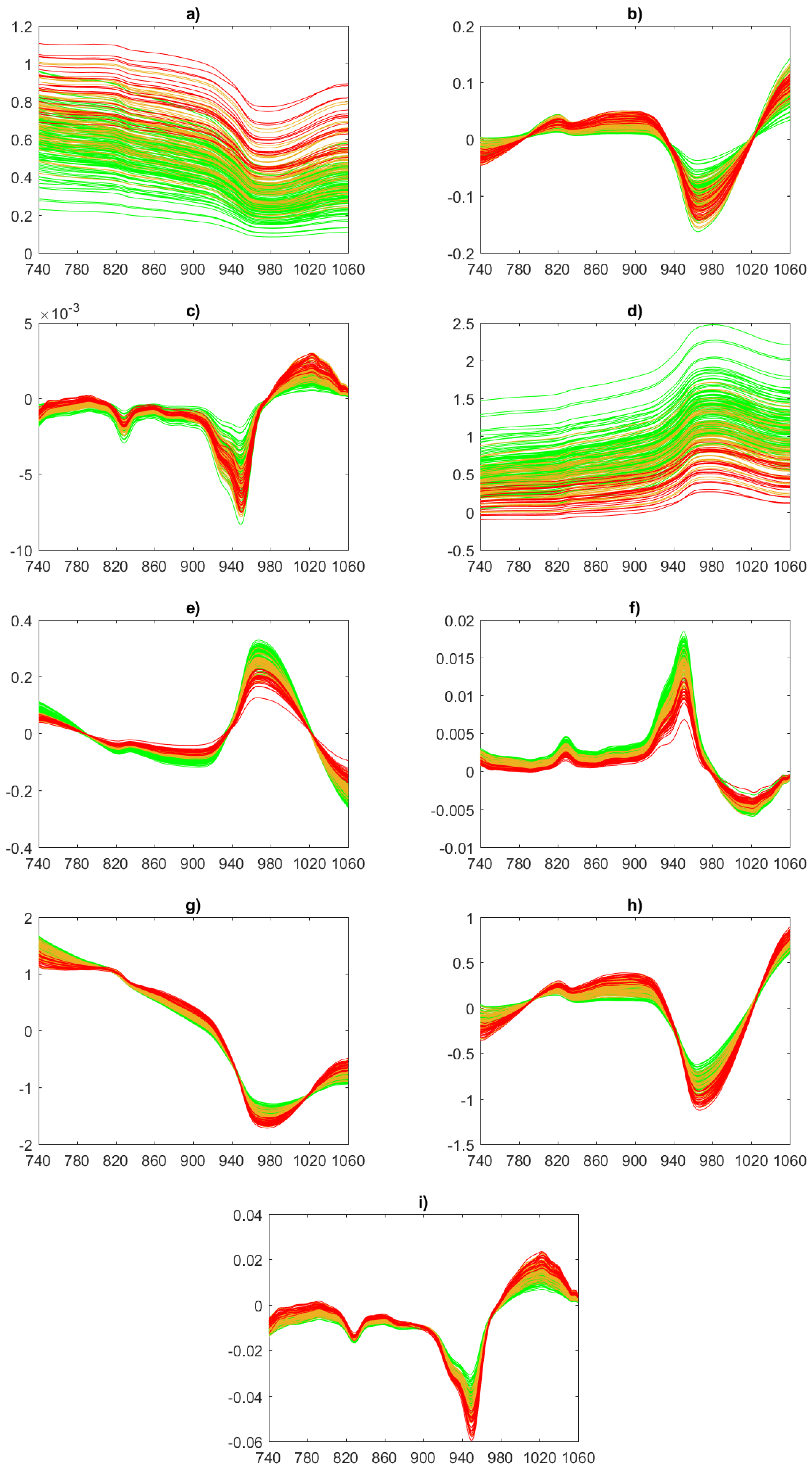
In this work, data preprocessing seeks to reduce the influence of any external phenomena which could have altered the spectra. Nevertheless, there is no universal approach and the most suitable one is chosen through an empirical process based on expertise [50,51]. Moreover, it is highly uncommon to use only a single preprocessing technique, due to each preprocessing technique providing complementary information. In Xu et al. [52], some combinations of preprocessing techniques were proposed to improve the stability of the models, which has been recently backed by other studies [53,54,55,56]. In this work, nine combinations of different techniques have been considered to preprocess the inputs. In Figure 2, the changes in the spectra for these nine combinations of preprocessing techniques are shown. The following are basic elements of these combinations:
  • Raw reflectance spectra directly obtained from the NIR-reflectance instrument without further preprocessing. This is the primary source of information in any NIR spectra [50].
  • The Beer–Lambert technique suggests a linear relationship between the concentration of a component and the absorbance of the spectra. The formula can be expressed as follows [50]:
    Aλ = −log10(R) ≅ ϵλlc
    where Aλ is the absorbance, R is the reflectance obtained by the NIR instrument, ϵλ is the wavelength-dependent molar absorptivity, l is the length of the light through the sample and c is the concentration of the component [50].
  • The aim of the detrending technique is to remove the baseline and the curvilinearity of the spectra. This method models the baseline as a linear function, which is then subtracted from each spectrum value independently [57].
  • Savitzky and Golay [58] popularized a method named after its authors, which consists of a smoothing function for the numerical derivation of a vector. In this method, a p-order polynomial is fitted and then the d-order derivative is calculated at center point i.
  • Standard normal variate (SNV) is a technique used for scattering correction [59]. This process can be expressed in the form of the following equation:
    Xi , snv = x ¯ S
    where Xi,snv is the SNV at a wavelength i, x ¯ is the spectrum average of the sample to be corrected, and S is the standard deviation of the spectrum sample.

3.2. Optimization of Model 1: Classification of Positive/Negative Samples

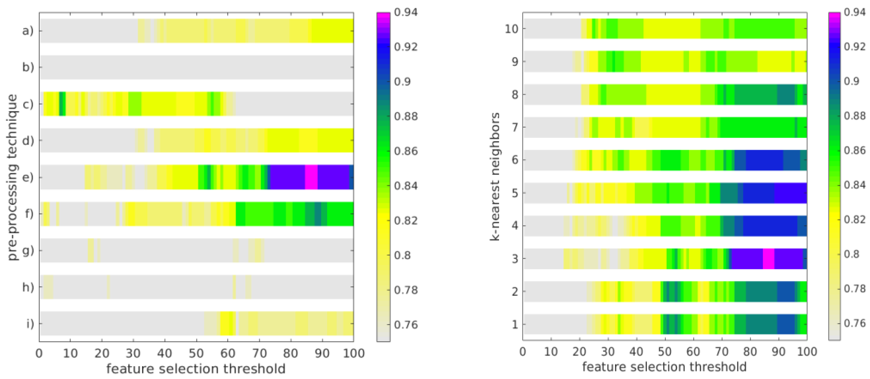
In the optimization of the first model, each one of the nine aforementioned preprocessing combinations was used as input, each at a time. The models use a kNN algorithm with 3 neighbors, and they were tested at different feature selection thresholds ranging from 0 to 100. The accuracy achieved by each configuration is shown in Figure 3 (left) where the maximum accuracy was obtained with a SNV preprocessing technique, and the feature selection threshold was between 11 and 18.
Once the preprocessing technique had been chosen, the second optimization process was performed. Its objective was to optimize the neighborhood size and the feature selection threshold. Models were tested with k-nearest neighbors between 1 and 10 and different feature selection thresholds from 0 to 100.
In Figure 3 (right), the accuracy of the model with different neighborhood sizes is shown. It should be highlighted that, with the SNV preprocessing technique, the model achieved accuracies above 0.84 with any of the k-nearest neighbors experimented. However, the best results were achieved when the model used six as number of nearest neighbors. On the other hand, accuracy is deeply affected by the feature selection threshold, since it sets the amount of input values received by the model. A feature selection threshold equal to 12 allowed the model to achieve the best results with 6 nearest neighbors.

3.3. Optimization of Model 2: Classification of Clinical/Subclinical Positive Samples

Again, the optimization of the second model starts by applying each of the nine aforementioned preprocessing combinations and using each of them as input. The models used a kNN with 3 neighbors, and they were tested at different feature selection thresholds between 0 and 100.
The accuracy achieved by each configuration of this second model can be seen in Figure 4 (left). In this case, the maximum accuracy was reached when the spectra were processed by the combination of applying the Beer–Lambert and then the detrending technique. Finally, the feature selection threshold was between 40 and 55.
Once the preprocessing technique was chosen, the second step sought to optimize the size of the neighborhood and feature selection threshold. Models were created with k-nearest neighbors from 1 to 10 neighbors and with different thresholds from 0 to 100.
Figure 4 (right) shows the accuracies of different configurations. As can be seen, good results were achieved with any number of neighbors between three and six. Using the selected preprocessing technique, the model yielded accuracy values above 0.83 with any value of k. However, the best results were achieved when the model used three nearest neighbors. Focusing the attention on the feature selection threshold, any value between 85 to 87 allowed model 2 to achieve the best results with 3 nearest neighbors.
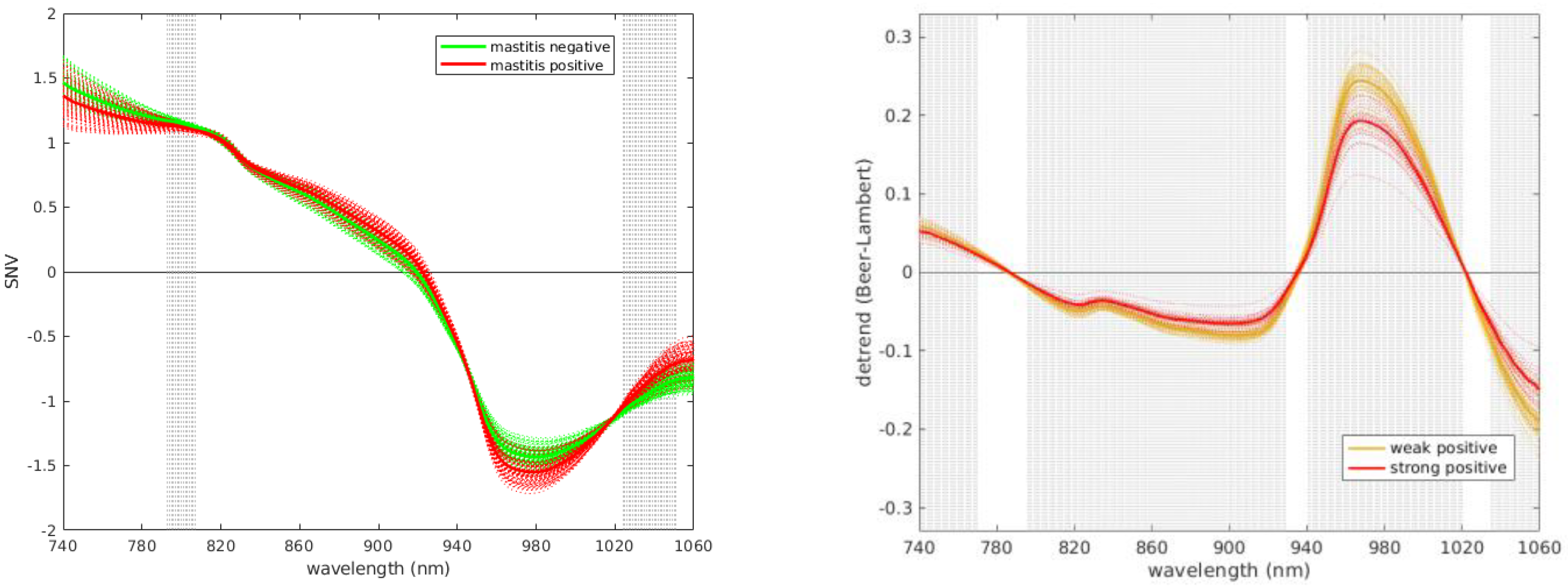
Processed NIR spectra and relevant wavelengths (shadowed) are shown in Figure 5. Notice the difference between the spectra of mastitis in negative and positive samples in Figure 5 (left). These differences were statistically significant (p < 0.05 t-test), with a feature selection between 11 and 18. Figure 5 (right) shows the combination of the Beer–Lambert and detrending techniques; the preprocessing technique made it possible to accurately classify athe mastitis positive milk samples as weak or strong positive—the differences between weak positive and strong positive samples were statistically significant (p < 0.05 t-test).

4. Discussion

High accuracies were achieved for both models, as shown in Table 2. According to Hamann & Krömker [14], these models detect changes in milk constituents which are related to mastitis. For example, levels of protein, chloride and sodium tend to increase along with SCC, while the levels of potassium and lactose tend to decrease.
In Jaeger et al. [60], the authors reported a SEN of 90.3% and an SPC of 71.8% in the detection of SCC, with the laboratory manual test showing the best results. Comparing these results with those reported in this work, we can see that there is no significant difference in sensitivity, considering the intervals reported in this work, while the specificity is significantly increased. Meilina et al. [19] reported another direct calculation method based on NIR spectra by simply using a double threshold to determine the presence of SCC. This work reported 77.78% and 80.56% for SEN and SPC, respectively, by using a lab grade NIR spectrometer and a comparison with the SCC. These results are summarized in Table 3, together with the comparative results of the proposed method and the details of the different datasets. It may be highlighted that some of the relevant data are not available from the sources.
Although Aernouts et al. [26] argue that short range spectrometers (400–1000) are not good enough for accurate monitoring the composition of raw milk, this study has proved that udder health can be estimated using a low-cost spectrometer which operates in a range close to the aforementioned equipment, with similar results to those obtained using laboratory methods.

Author Contributions

Conceptualization, I.R.-M. and D.R.; methodology, E.F.-B.; software, I.R.-M.; validation, I.R.-M., J.P. and L.A.; formal analysis, L.A.; investigation, L.A.; resources, J.P. and A.P.; data curation, I.R.-M.; writing—original draft preparation, I.R.-M.; writing—review and editing, E.F.-B.; visualization, D.R.; supervision, A.P.; project administration, J.P.; funding acquisition, J.P. and A.P. All authors have read and agreed to the published version of the manuscript.

Funding

This work is part of DINTA-UTMACH and RNASA-UDC research groups. This work is partially supported by Instituto de Salud Carlos III, grant number PI17/01826. It was also partially supported by different grants and projects from the Xunta de Galicia [ED431D 2017/23; ED431D 2017/16; ED431G/01; ED431C 2018/49; IN845D-2020/03]. Another source of support was the CYTED network (PCI2018\_093284) funded by the Spanish Ministry of Innovation and Science.

Data Availability Statement

Dataset [61] will be publicly available after the manuscript is accepted, during the reviewing process, the dataset is available for downloading at the following private link: https://data.mendeley.com/datasets/mj8wcb9fsd/draft?a=f457ba3f-3005-4153-97b3-048edfb4027f (accessed on 8 September 2021).

Acknowledgments

The authors wish to thank the CESGA Supercomputing Center, where most of the experiments were performed. Also a special thanks to Karen Jimenez and Yajaira Obando, for their help while sampling milk using CMT and NIR when they were undergraduate students. Iván Ramírez-Morales Daniel Rivero and Enrique Fernández-Blanco would also like to give thanks for the support provided by the NVIDIA Research Grants Program.

Conflicts of Interest

The authors declare no conflict of interest.

References

  1. Sharma, N.; Rho, G.J.; Hong, Y.H.; Kang, T.Y.; Lee, H.K.; Hur, T.Y.; Jeong, D.K. Bovine Mastitis: An Asian Perspective. Asian J. Anim. Vet. Adv. 2012, 7, 454–476. [Google Scholar] [CrossRef] [Green Version]
  2. Sudhan, N.A.; Sharma, N. Mastitis-an Important Production Disease of Dairy Animals. In SMVS Dairy Year Book; SMVS: Ghaziabad, India, 2010; pp. 72–88. [Google Scholar]
  3. León-Galván, M.F.; Barboza-Corona, J.E.; Lechuga-Arana, A.A.; Valencia-Posadas, M.; Aguayo, D.D.; Cedillo-Pelaez, C.; Martínez-Ortega, E.A.; Gutierrez-Chavez, A.J. Molecular Detection and Sensitivity to Antibiotics and Bacteriocins of Pathogens Isolated from Bovine Mastitis in Family Dairy Herds of Central Mexico. BioMed Res. Int. 2015, 2015, 615153. [Google Scholar] [CrossRef]
  4. Hogeveen, H.; Huijps, K.; Lam, T.J.G.M. Economic Aspects of Mastitis: New Developments. N. Z. Vet. J. 2011, 59, 16–23. [Google Scholar] [CrossRef]
  5. Schroeder, J.W. Bovine Mastitis and Milking Management. Drug Ther. 2012, 8, 4. [Google Scholar]
  6. Dohoo, I.R.; Smith, J.; Andersen, S.; Kelton, D.F.; Godden, S. Mastitis Research Workers’ Conference Diagnosing Intramammary Infections: Evaluation of Definitions Based on a Single Milk Sample. J. Dairy Sci. 2011, 94, 250–261. [Google Scholar] [CrossRef] [Green Version]
  7. Zimmer, M. A Comparison between the DHIA Test for Somatic Cell Counts Compared to Porta Side Test on the Individual Quarters of the High SCC Cows at the Cal Poly Dairy; California Polytechnic State University: San Luis Obispo, CA, USA, 2010. [Google Scholar]
  8. Janik, I.A. The Detection and Prediction of Mastitis in Dairy Cows by Particle Analysis. Ph.D. Thesis, Coventry University, Coventry, UK, 2013. [Google Scholar]
  9. Perrin, G.G.; Mallereau, M.P.; Lenfant, D.; Baudry, C. Relationships between California Mastitis Test (CMT) and Somatic Cell Counts in Dairy Goats. Small Rumin. Res. 1997, 26, 167–170. [Google Scholar] [CrossRef]
  10. Shitandi, A.; Kihumbu, G. Assessment of the California Mastitis Test Usage in Smallholder Dairy Herds and Risk of Violative Antimicrobial Residues. J. Vet. Sci. 2004, 5, 5–9. [Google Scholar] [CrossRef] [Green Version]
  11. Schalm, O.W.; Noorlander, D.O. Experiments and Observations Leading to Development of the California Mastitis Test. J. Am. Vet. Med. Assoc. 1957, 130, 199–204. [Google Scholar]
  12. McDougall, S.; Murdough, P.; Pankey, W.; Delaney, C.; Barlow, J.; Scruton, D. Relationships among Somatic Cell Count, California Mastitis Test, Impedance and Bacteriological Status of Milk in Goats and Sheep in Early Lactation. Small Rumin. Res. 2001, 40, 245–254. [Google Scholar] [CrossRef]
  13. Viguier, C.; Arora, S.; Gilmartin, N.; Welbeck, K.; O’Kennedy, R. Mastitis Detection: Current Trends and Future Perspectives. Trends Biotechnol. 2009, 27, 486–493. [Google Scholar] [CrossRef]
  14. Hamann, J.; Krömker, V. Potential of Specific Milk Composition Variables for Cow Health Management. Livest. Prod. Sci. 1997, 48, 201–208. [Google Scholar] [CrossRef]
  15. Kaur, H. Counterfeit Pharmaceuticals and Methods to Test Them. In Annual Report of the Government Chief Scientific Adviser 2015: Forensic Science and Beyond: Authenticity, Provenance and Assurance Evidence and Case Studies; Walport, M., Ed.; Government Office for Science: London, UK, 2015; pp. 132–137. [Google Scholar]
  16. Guillemain, A.; Dégardin, K.; Roggo, Y. Performance of NIR Handheld Spectrometers for the Detection of Counterfeit Tablets. Talanta 2017, 165, 632–640. [Google Scholar] [CrossRef]
  17. Weesepoel, Y.J.A.; van Ruth, S.M. Miniaturized NIRs for Age and Expiration Date Prediction of Packaged Chicken Fillets; Academic: Cambridge, MA, USA, 2016. [Google Scholar]
  18. Holroyd, S.E. The Use of near Infrared Spectroscopy on Milk and Milk Products. J. Near Infrared Spectrosc. 2013, 21, 311–322. [Google Scholar] [CrossRef]
  19. Meilina, H.; Kuroki, S.; Jinendra, B.M.; Ikuta, K.; Tsenkova, R. Double Threshold Method for Mastitis Diagnosis Based on NIR Spectra of Raw Milk and Chemometrics. Biosyst. Eng. 2009, 104, 243–249. [Google Scholar] [CrossRef]
  20. Veleva-Doneva, P.; Draganova, T.; Atanassova, S.; Tsenkova, R. Detection of Bacterial Contamination in Milk Using NIR Spectroscopy and Two Classification Methods—SIMCA and Neuro—Fuzzy Classifier. IFAC Proc. Vol. 2010, 43, 225–229. [Google Scholar] [CrossRef]
  21. Russell, A. Milk Spectroscopy. Master’s Thesis, The University of Waikato, Hamilton, New Zealand, 2013. [Google Scholar]
  22. Tsenkova, R.; Atanassova, S.; Ozaki, Y.; Toyoda, K.; Itoh, K. Near-Infrared Spectroscopy for Biomonitoring: Influence of Somatic Cell Count on Cow’s Milk Composition Analysis. Int. Dairy J. 2001, 11, 779–783. [Google Scholar] [CrossRef]
  23. Wilson, B.K.; Kaur, H.; Allan, E.L.; Lozama, A.; Bell, D. A New Handheld Device for the Detection of Falsified Medicines: Demonstration on Falsified Artemisinin-Based Therapies from the Field. Am. J. Trop. Med. Hyg. 2017, 96, 1117. [Google Scholar] [CrossRef] [Green Version]
  24. Vanderroost, M.; Ragaert, P.; Verwaeren, J.; De Meulenaer, B.; De Baets, B.; Devlieghere, F. The Digitization of a Food Package’s Life Cycle: Existing and Emerging Computer Systems in the Logistics and Post-Logistics Phase. Comput. Ind. 2017, 87, 15–30. [Google Scholar] [CrossRef]
  25. Rateni, G.; Dario, P.; Cavallo, F. Smartphone-Based Food Diagnostic Technologies: A Review. Sensors 2017, 17, 1453. [Google Scholar] [CrossRef]
  26. Aernouts, B.; Polshin, E.; Lammertyn, J.; Saeys, W. Visible and near-Infrared Spectroscopic Analysis of Raw Milk for Cow Health Monitoring: Reflectance or Transmittance? J. Dairy Sci. 2011, 94, 5315–5329. [Google Scholar] [CrossRef] [Green Version]
  27. Ozcan, A. Mobile Phones Democratize and Cultivate next-Generation Imaging, Diagnostics and Measurement Tools. Lab Chip 2014, 14, 3187–3194. [Google Scholar] [CrossRef]
  28. Brasil, Y.L.; Cruz-Tirado, J.P.; Barbin, D.F. Fast Online Estimation of Quail Eggs Freshness Using Portable NIR Spectrometer and Machine Learning. Food Control 2022, 131, 108418. [Google Scholar] [CrossRef]
  29. Cruz-Tirado, J.P.; da Silva Medeiros, M.L.; Barbin, D.F. On-Line Monitoring of Egg Freshness Using a Portable NIR Spectrometer in Tandem with Machine Learning. J. Food Eng. 2021, 306, 110643. [Google Scholar] [CrossRef]
  30. Wu, X.; Kumar, V.; Quinlan, J.R.; Ghosh, J.; Yang, Q.; Motoda, H.; McLachlan, G.J.; Ng, A.; Liu, B.; Yu, P.S.; et al. Top 10 Algorithms in Data Mining. Knowl. Inf. Syst. 2008, 14, 1–37. [Google Scholar] [CrossRef] [Green Version]
  31. Goldring, D.; Sharon, D.; Brodetzki, G.; Ruf, A. Withdrawn Patent as Per the Latest Uspto Withdrawn List. US Patent US10704954B2, 7 July 2020. [Google Scholar]
  32. Quinn, P.J.; Carter, M.E.; Morley, B.; Carter, G.R. Bovine Mastitis and Antibiotic Resistance Patterns in Selalle Smallholder Dairy Farms, Central Ethiopia. Clin. Vet. Microbiol. 1994, 1, 861–868. [Google Scholar] [CrossRef]
  33. Amer, S.; Gálvez, F.L.A.; Fukuda, Y.; Tada, C.; Jimenez, I.L.; Valle, W.F.M.; Nakai, Y. Prevalence and Etiology of Mastitis in Dairy Cattle in El Oro Province, Ecuador. J. Vet. Med. Sci. 2018, 80, 861–868. [Google Scholar] [CrossRef] [Green Version]
  34. Mucherino, A.; Papajorgji, P.J.; Pardalos, P.M. Data Mining in Agriculture; Springer Optimization and Its Applications; Springer: New York, NY, USA, 2009; Volume 34, pp. 143–160. ISBN 9780387886145. [Google Scholar]
  35. Blanco, M.; Villarroya, I. NIR Spectroscopy: A Rapid-Response Analytical Tool. Trends Analyt. Chem. 2002, 21, 240–250. [Google Scholar] [CrossRef]
  36. Guyon, I.; Gunn, S.; Nikravesh, M.; Zadeh, L.A. Feature Extraction: Foundations and Applications; Studies in Fuzziness and Soft Computing; Springer: Berlin/Heidelberg, Germany, 2008; ISBN 9783540354888. [Google Scholar]
  37. Chandrashekar, G.; Sahin, F. A Survey on Feature Selection Methods. Comput. Electr. Eng. 2014, 40, 16–28. [Google Scholar] [CrossRef]
  38. Saeys, Y.; Inza, I.; Larrañaga, P. A Review of Feature Selection Techniques in Bioinformatics. Bioinformatics 2007, 23, 2507–2517. [Google Scholar] [CrossRef] [Green Version]
  39. Szymańska, E.; Gerretzen, J.; Engel, J.; Geurts, B.; Blanchet, L.; Buydens, L.M.C. Chemometrics and Qualitative Analysis Have a Vibrant Relationship. Trends Analyt. Chem. 2015, 69, 34–51. [Google Scholar] [CrossRef]
  40. Hall, M.A. Correlation-Based Feature Selection for Machine Learning. Ph.D. Thesis, The University of Waikato, Hamilton, New Zealand, 1999. [Google Scholar]
  41. Kim, J.; Ko, J.; Choi, H.; Kim, H. Printed Circuit Board Defect Detection Using Deep Learning via A Skip-Connected Convolutional Autoencoder. Sensors 2021, 21, 4968. [Google Scholar] [CrossRef]
  42. Bishop, C.M. Pattern Recognition and Machine Learning; Springer: Berlin/Heidelberg, Germany, 2006; ISBN 9780387310732. [Google Scholar]
  43. Mucherino, A.; Ruß, G. Recent Developments in Data Mining and Agriculture. In Proceedings of the Industrial Conference on Data Mining-Workshops, New York, NY, USA, 30 August–3 September 2011; pp. 90–98. [Google Scholar]
  44. Cawley, G.C.; Talbot, N.L. On over-Fitting in Model Selection and Subsequent Selection Bias in Performance Evaluation. J. Mach. Learn. Res. 2010, 11, 2079–2107. [Google Scholar]
  45. Fawcett, T. An Introduction to ROC Analysis. Pattern Recognit. Lett. 2006, 27, 861–874. [Google Scholar] [CrossRef]
  46. Altman, D.G.; Bland, J.M. Diagnostic Tests 2: Predictive Values. BMJ 1994, 309, 102. [Google Scholar] [CrossRef] [Green Version]
  47. Hastie, T.; Tibshirani, R.; Friedman, J. The Elements of Statistical Learning: Data Mining, Inference, and Prediction, 2nd ed.; Springer Science & Business Media: Berlin/Heidelberg, Germany, 2009; ISBN 9780387848587. [Google Scholar]
  48. Müller, A.C.; Guido, S. Introduction to Machine Learning with Python: A Guide for Data Scientists; O’Reilly Media, Inc.: Sebastopol, CA, USA, 2016; ISBN 9781449369903. [Google Scholar]
  49. Ma, X.; Zhang, Y.; Wang, Y. Performance Evaluation of Kernel Functions Based on Grid Search for Support Vector Regression. In Proceedings of the 2015 IEEE 7th International Conference on Cybernetics and Intelligent Systems (CIS) and IEEE Conference on Robotics, Automation and Mechatronics (RAM), Siem Reap, Cambodia, 15–17 July 2015; pp. 283–288. [Google Scholar]
  50. Rinnan, Å.; van Berg, F.D.; Engelsen, S.B. Review of the Most Common Pre-Processing Techniques for near-Infrared Spectra. Trends Analyt. Chem. 2009, 28, 1201–1222. [Google Scholar] [CrossRef]
  51. dos Santos, C.A.T.; Lopo, M.; Páscoa, R.N.M.J.; Lopes, J.A. A Review on the Applications of Portable near-Infrared Spectrometers in the Agro-Food Industry. Appl. Spectrosc. 2013, 67, 1215–1233. [Google Scholar] [CrossRef]
  52. Xu, L.; Zhou, Y.-P.; Tang, L.-J.; Wu, H.-L.; Jiang, J.-H.; Shen, G.-L.; Yu, R.-Q. Ensemble Preprocessing of near-Infrared (NIR) Spectra for Multivariate Calibration. Anal. Chim. Acta 2008, 616, 138–143. [Google Scholar] [CrossRef]
  53. Martelo-Vidal, M.J.; Vázquez, M. Evaluation of Ultraviolet, Visible, and near Infrared Spectroscopy for the Analysis of Wine Compounds. Czech J. Food Sci. 2014, 32, 37. [Google Scholar] [CrossRef] [Green Version]
  54. Xie, L.; He, X.; Duan, B.; Tang, S.; Luo, J.; Jiao, G.; Shao, G.; Wei, X.; Sheng, Z.; Hu, P. Optimization of Near-Infrared Reflectance Model in Measuring Gelatinization Characteristics of Rice Flour with a Rapid Viscosity Analyzer (RVA) and Differential Scanning Calorimeter (DSC). Cereal Chem. 2015, 92, 522–528. [Google Scholar] [CrossRef]
  55. Hadad, G.M.; Ra, A.S.; Elkhoudarya, M.M. Simultaneous Determination of Clarithromycin, Tinidazole and Omeprazole in Helicure Tablets Using Reflectance Near-Infrared Spectroscopy with the Aid of Chemometry. Pharm. Anal. Acta 2015, 2015. [Google Scholar] [CrossRef] [Green Version]
  56. Ramírez-Morales, I.; Rivero, D.; Fernández-Blanco, E.; Pazos, A. Optimization of NIR Calibration Models for Multiple Processes in the Sugar Industry. Chemom. Intellig. Lab. Syst. 2016, 159, 45–57. [Google Scholar] [CrossRef]
  57. Luypaert, J.; Heuerding, S.; de Jong, S.; Massart, D.L. An Evaluation of Direct Orthogonal Signal Correction and Other Preprocessing Methods for the Classification of Clinical Study Lots of a Dermatological Cream. J. Pharm. Biomed. Anal. 2002, 30, 453–466. [Google Scholar] [CrossRef]
  58. Savitzky, A.; Golay, M.J.E. Smoothing and Differentiation of Data by Simplified Least Squares Procedures. Anal. Chem. 1964, 36, 1627–1639. [Google Scholar] [CrossRef]
  59. Barnes, R.J.; Dhanoa, M.S.; Lister, S.J. Standard Normal Variate Transformation and De-Trending of Near-Infrared Diffuse Reflectance Spectra. Appl. Spectrosc. 1989, 43, 772–777. [Google Scholar] [CrossRef]
  60. Jaeger, S.; Virchow, F.; Torgerson, P.R.; Bischoff, M.; Biner, B.; Hartnack, S.; Rüegg, S.R. Test Characteristics of Milk Amyloid A ELISA, Somatic Cell Count, and Bacteriological Culture for Detection of Intramammary Pathogens That Cause Subclinical Mastitis. J. Dairy Sci. 2017, 100, 7419–7426. [Google Scholar] [CrossRef] [Green Version]
  61. Ramirez-Morales, I. NIR Spectral Signal of Healthy and Mastitic Milk Samples. Mendeley Data 2021, 1. [Google Scholar] [CrossRef]
Figure 1. Nested-leave-one-cow-out cross-validation approach used in this work.
Applsci 11 10751 g001
Figure 2. Changes in spectral signal of raw milk samples according to the preprocessing combinations used in this work (a) raw spectra, (b) detrended raw spectra, (c) Savitzky–Golay applied to raw spectra, (d) Beer–Lambert law (BL) applied to raw spectra, (e) detrending applied to BL, (f) Savitzky–Golay applied to BL, (g) standard normal variate (SNV) applied to raw spectra, (h) detrending applied to SNV, (i) Savitzky–Golay applied to SNV.
Applsci 11 10751 g002
Figure 3. Accuracy of a k-NN model 1 in leave-one-cow-out nested cross-validation: with 3 neighbors, according to the preprocessing combinations described in Figure 2 (letters from a to i) and feature threshold (left), with different values of k-nearest neighbors, and feature selection thresholds (right).
Applsci 11 10751 g003
Figure 4. Accuracy of k-NN model 2 in nested-leave-one-cow-out cross-validation: with 3 neighbors, according to the preprocessing combinations described in Figure 2 (letters from a to i) and feature threshold (left), with different values of k-nearest neighbors, and feature selection thresholds (right).
Applsci 11 10751 g004
Figure 5. Processed spectra and relevant bands: SNV for model 1 (left), detrend and Beer–Lambert for model 2 (right).
Applsci 11 10751 g005
Table 1. Interpretation of results of CMT and grouping for classification algorithm.
CMTInterpretationClassNumber of Samples
0NegativeNegative130
+TraceWeak Positive57
++Weak positive
+++Distinctive positiveStrong Positive23
++++Strong positive
Table 2. Performance metrics of models on the test set, 10-fold nested cross-validation.
Performance MetricModel 1: Positive—NegativeModel 2: Clinical—Subclinical
Accuracy x ¯ = 0.912 σ = 0.051 x ¯ = 0.951 σ = 0.08
Sensitivity x ¯ = 0.858 σ = 0.129 x ¯ = 0.95 σ = 0.158
Specificity x ¯ = 0.94 σ = 0.064 x ¯ = 0.957 σ = 0.096
Positive Predictive Value x ¯ = 0.89 σ = 0.11 x ¯ = 0.917 σ = 0.18
Negative Predictive Value x ¯ = 0.925 σ = 0.072 x ¯ = 0.978 σ = 0.07
F1 Score x ¯ = 0.867 σ = 0.089 x ¯ = 0.913 σ = 0.144
Table 3. Comparison of datasets used for mastitis detection using NIR spectra.
WorkDatasetPositive CasesPublicValidation MethodSensitivitySpecificity
Jaeger et al. [60]433275No-90.3%71.8%
Meilina et al. [19]666-No-77.8%80.6%
This work21080YesLOOCV85.8%94.0%
Publisher’s Note: MDPI stays neutral with regard to jurisdictional claims in published maps and institutional affiliations.