Abstract
In this paper, a Lie-algebraic nonholonomic motion planning technique, originally designed to work in a configuration space, was extended to plan a motion within a task-space resulting from an output function considered. In both planning spaces, a generalized Campbell–Baker–Hausdorff–Dynkin formula was utilized to transform a motion planning into an inverse kinematic task known for serial manipulators. A complete, general-purpose Lie-algebraic algorithm is provided for a local motion planning of nonholonomic systems with or without output functions. Similarities and differences in motion planning within configuration and task spaces were highlighted. It appears that motion planning in a task-space can simplify a planning task and also gives an opportunity to optimize a motion of nonholonomic systems. Unfortunately, in this planning there is no way to avoid working in a configuration space. The auxiliary objective of the paper is to verify, through simulations, an impact of initial parameters on the efficiency of the planning algorithm, and to provide some hints on how to set the parameters correctly.
1. Introduction
A large number of contemporary and practically important robots can be described as nonholonomic systems. Despite different sources of nonholonomy and nonholonomic manipulators, wheel mobile robots [1] and free-floating space robots [2] belong to this class. Even when modeled at the kinematic level, nonholonomic systems are difficult to control because the number of controls is smaller than the dimension of their configuration spaces. Thus, sophisticated maneuvers have to be performed to get a desired location, clearly exemplified by the task of parking a car (especially towing trailers). For some special cases of nonholonomic systems (like Dubbins [3] and Reeds-Shepp cars [4] or systems in a chain form [5]), dedicated methods were proposed to plan their motions. However, there is a constant need to develop general purpose methods applicable to any nonholonomic system. Two main classes of general purpose methods can be distinguished: global [6,7] and local ones [8]. Global methods try to get a whole output trajectory at once (although in an iterative manner), while local ones construct an output trajectory from sub-trajectories derived from local planning. Global methods are rooted in various paradigms. Using a linearization of a nonholonomic system along the trajectory corresponding to current controls, Tchon and coworkers [7] reformulated a nonholonomic motion planning task into an inverse task solved with classical methods. Jakubczyk [9] applied the Volterra series expansion of a nonholonomic system with an output function to get highly oscillatory controls that were able to trace a desired trajectory with an arbitrary precision. Arismendi and coworkers [10] adapted a variant of a wave front technique to design the fast marching square path planning method of nonholonomic motion planning.
Generally, algorithms derived from global methods are computationally involved and very sensitive to geometric constraints due to obstacles. Consequently, they cannot be applied in dynamic or partially unknown environments. Local methods do not suffer from these drawbacks.
In this paper, a Lie-algebraic local method of motion planning will be studied. There are three main goals of the paper:
- to extend applicability of the method to plan a motion also within a task-space, and to provide a complete algorithm for implementing the method,
- to show through simulations how data parameterizing the algorithm impacts its efficiency,
- to compare planning within a configuration and a task-space, pointing out similarities and differences.
It is worth noticing that local and global planning tasks belong to a classic triple: geometrical planning, motion planning, and control. Recently, some attempts have been made to combine the last two tasks into one planning-control loop [11,12]. A vast majority of motion planning algorithms are based on discretization of control/configuration spaces to transform continuous tasks, described by differential equations and static output functions, into a graph domain. In this discrete space, graph-searching algorithms, like RRT or its numerous variants [13], can be used to solve the planning task.
The paper is organized as follows: In Section 2 a model of nonholonomic systems is introduced supplemented with an output function, then a motion planning task is defined and, finally, a Lie algebraic algorithm to solve the task is presented. In Section 3 an extensive simulation study is provided to evaluate performance of the algorithm for various data that impact its behavior. Then, some observations are formulated based on the simulation results. Section 4 concludes the paper.
2. Model and Algorithm
Nonholonomic systems modeled at a kinematic level are described by the control-affine equation [14]
where is a configuration, are controls, and are (smooth) vector fields (generators) that span a null space of nonholonomic constraints. By definition, nonholonomic systems satisfy the Lie algebra rank condition. Thus, according to the Chow’s theorem [15], they are small time locally controllable.
In order to shorten notations, two-input systems, , will be considered with and . Two input systems are the most challenging as for the systems it is quite easy to generate difficult motion planning tasks by increasing a configuration space dimension.
In many practical applications not all components of a configuration vector are important (for example wheel angles of mobile robots do not impact obstacle collisions), thus an output map is introduced
and usually .
Now, a motion planning task can be stated as follows: given an initial configuration and a goal point, find controls which, applied to the system (1), generates an end-point of the resulting trajectory mapped with Equation (2) into the desired location .
In Lie-algebraic methods, locally, around a current configuration , possible directions of motion of the system (1) are described by vector fields derived from generators . To avoid redundancy, it is a common practice to take only a basis of the Lie algebra spanned by the generators. There are at least three such bases, but probably the most frequently used is the Ph. Hall basis. It is composed of an infinite number of Lie monomials, interpreted as vector fields within the scope of the control system (1). The very first elements of the basis are given below
where denotes a Lie bracket of Lie monomials (for vector fields ). The basis is composed of generators (degree 1 Lie monomials) and higher degree monomials derived from generators and their descendants. The system (1) is a nonholonomic one, thus a finite (and usually small) number of initial Ph. Hall basis elements, , can be taken to satisfy the Lie algebra rank condition [15]
Consequently, the system (1) is a small time locally controllable and it can evolve at any configuration in any direction. The condition (4) is quite easy to check in off-line mode with the assistance of symbolic computation packages. However, a very demanding problem is how to generate a motion in any direction with a small number of controls. Fortunately, the generalized Campbell–Baker–Hausdorff–Dynkin formula [16] answers this question constructively. It states that a configuration shift at a current configuration , depends on controls [17] as follows
where control-dependent coefficients pre-multiplying Lie monomials (vector fields) are expressed as
and they become more and more complex as the integration is performed over the k-dimensional simplex, where k is the degree of a Lie monomial the coefficient corresponds to. It is a common practice to express controls as linear combinations of time-dependent functions [7]
where are elements of any functional basis (polynomials, harmonic functions) and is the number of variables required to describe the i-th control. Thus, a vector collects all variables and uniquely describes controls and also energy of controls. Moreover, the shift (5) can be expressed as a function of and resembles forward kinematics (but at a velocity level when considered on a fixed time horizon)
The shift (8) from the configuration space is mapped into the task-space, and within this space a desired motion towards the goal can be computed using the Newton algorithm. A complete algorithm to plan a motion of the system (1) with the output function (2), either in a configuration or a task-space, is presented in Algorithm 1.
| Algorithm 1 nonholonomic motion planning within a task-space |
| Step 1. Read-in initial data: the system (1) together with the output function (2), the initial configuration and the goal point , desired accuracy of reaching the goal , the initial value of . Step 2. Initialize empty resulting trajectory , and set the current configuration . Step 3. Check the stop condition: iff then stop computations and output resulting trajectory . Otherwise, progress with Step 4. Step 4. Select a parameterization of controls (7), a time horizon T, and derive mapping (8). Step 5. At a current point in the task-space , select the planned shift by setting a positive coefficient . Step 6. Using the Newton algorithm, Ref. [18] find that solves the inverse kinematic task where is the Jacobi matrix of the mapping (2). Step 7. Check whether the solution is acceptable: where is the end-point of the trajectory initialized at and generated by the system (1) with controls , , corresponding to the vector of parameters , cf. Equation (7). Step 8. If Condition (12) is satisfied, then:
Otherwise, decrease the coefficient and go to Step 5. |
Comments on Algorithm 1:
- A nonholonomic motion planning in a configuration space is achieved by setting the identity output function (2).
- In Step 7, a minimal requirement was formulated, i.e., a new end-point of trajectory in the task-space should be closer to the goal than it was in the previous iteration. More restrictive requirement assumes that it should also be close enough to the planned sub-goal .
- Singularities in solving (11) result from a rank deficiency of the Jacobi matrix, derived from the right hand side of (11)Thus, singularities may arise
- either due to a rank deficiency of (they are avoidable by a small variation of controls which results in a small shift of )
- In Step 5, the positive coefficient should not be too large, as values of matrices , are computed at the current configuration and neglecting some vector fields, while truncation , is justified only locally. Its value cannot be too small either, as many iterations might be required to complete the algorithm.
- In motion planning within a task-space with , it is impossible to avoid planning within a configuration space, as the mapping (2) is not unique in this case.
3. Simulations
In order to evaluate Algorithm 1, some tests were performed using two models of mobile robots depicted in Figure 1. The unicycle is described by equations

Figure 1.
The unicycle (left panel) and the kinematic car (right panel).
The configuration vector is composed of position and orientation of the vehicle on a plane, while denote controls interpreted as angular and linear velocities.
The model of a kinematic car is given as
where configuration has got an extra component describing the steering wheel angle. For simplicity, it was assumed that . Both models are nonholonomic ones because generators supplemented with the Lie bracket for the unicycle
and
for the kinematic car, satisfy Condition (4).
For both models, the position on the xy plane was selected as the output function
If a robot is inscribed in a circle of sufficient radius, its orientation does not influence the possibility of collisions with obstacles. For the kinematic car another output function was used, coupling position on the xy plane and orientation of the vehicle
In practice, the orientation of the steering axle is not relevant. In order to check the motion planning Algorithm 1 within a configuration space, the identity output function was selected for both mobile robots.
In all tested cases, an initial configuration was set to the vector composed of zeroes only
In the tests, a side-way motion maneuver on the -plane was planned for both models and all output functions. The maneuver is challenging as it requires a motion along higher (than generators ) degree vector fields. Depending on a dimension of a task-space, goal points were selected as
Any single task was run using three parameterizations of controls. Each control was composed of a few very first items of the orthonormal Fourier basis
where and . Later on, it was assumed that . The total energy expenditure on controls is equal to
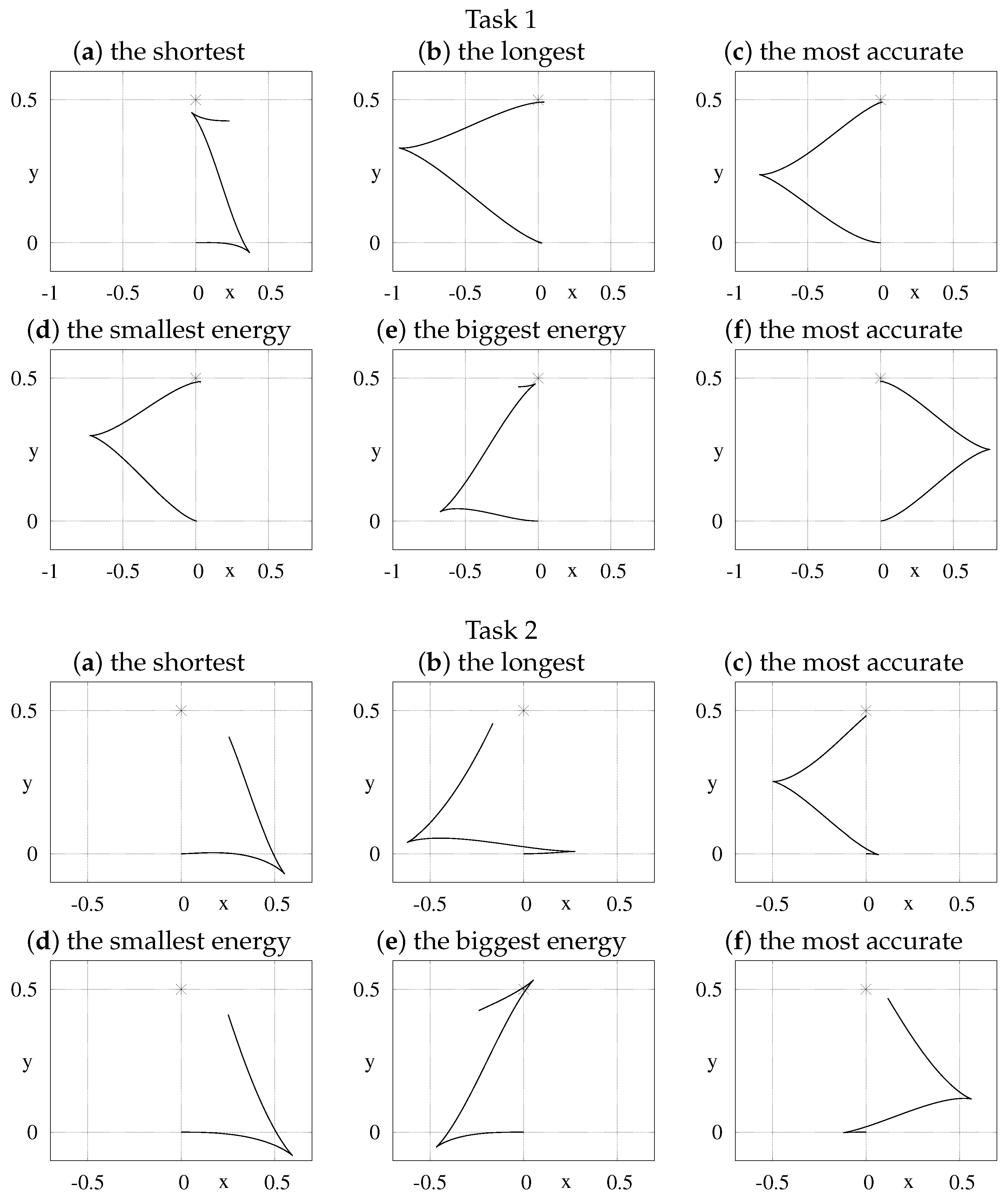
where is the number of the Fourier basis elements contributing to the i-th control. All tasks, with the data collected in Table 1, were solved using Algorithm 1. In Step 6 of the algorithm, two versions of the Newton algorithm were tested: the basic one and with the energy (25) optimization within the null-space of the Jacobi matrix (13). In order to obtain statistically significant results, Step 6 was repeated 100 times for each task, with initial values of varied (each component of was generated randomly with the uniform distribution on the interval ). Programs used in simulations were written in Wolfram Mathematica, version 11.3, and run on a computer with Intel® Core™ i5-8400 CPU and 24 GiB RAM memory. In Figure 2 and Figure 3, some characteristic paths (projected on the xy-plane and with a target point marked with an asterisk) were visualized for the unicycle and the kinematic car, respectively.

Table 1.
Data for tasks.
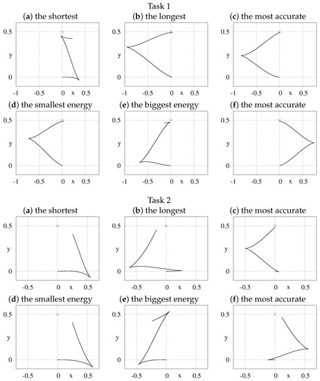

Figure 2.
xy-plane projections of some paths generated with basic (a–c) and null-space optimization (d–f) versions of the Newton algorithm run for the unicycle robot.

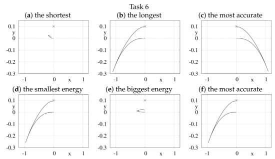
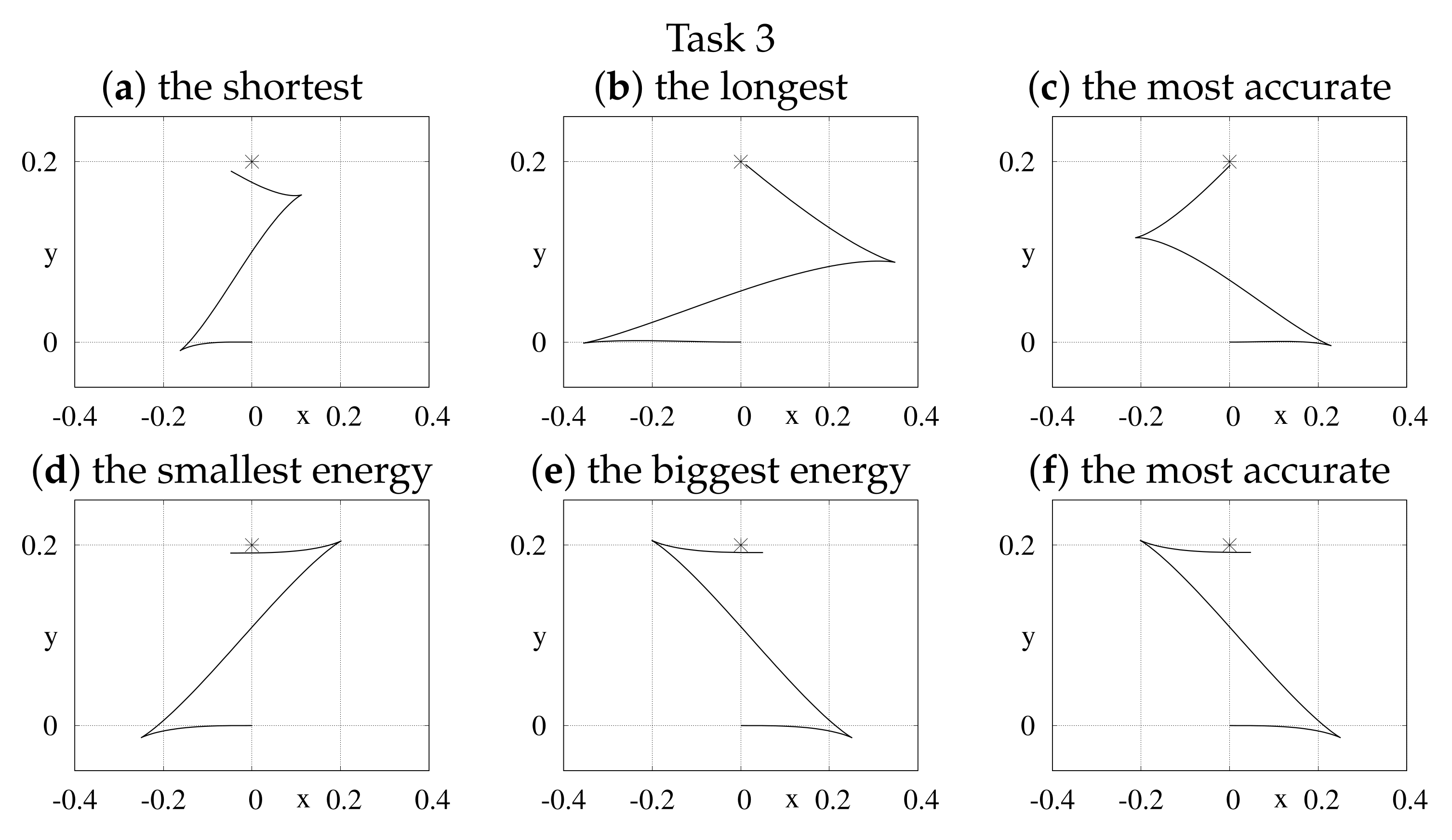
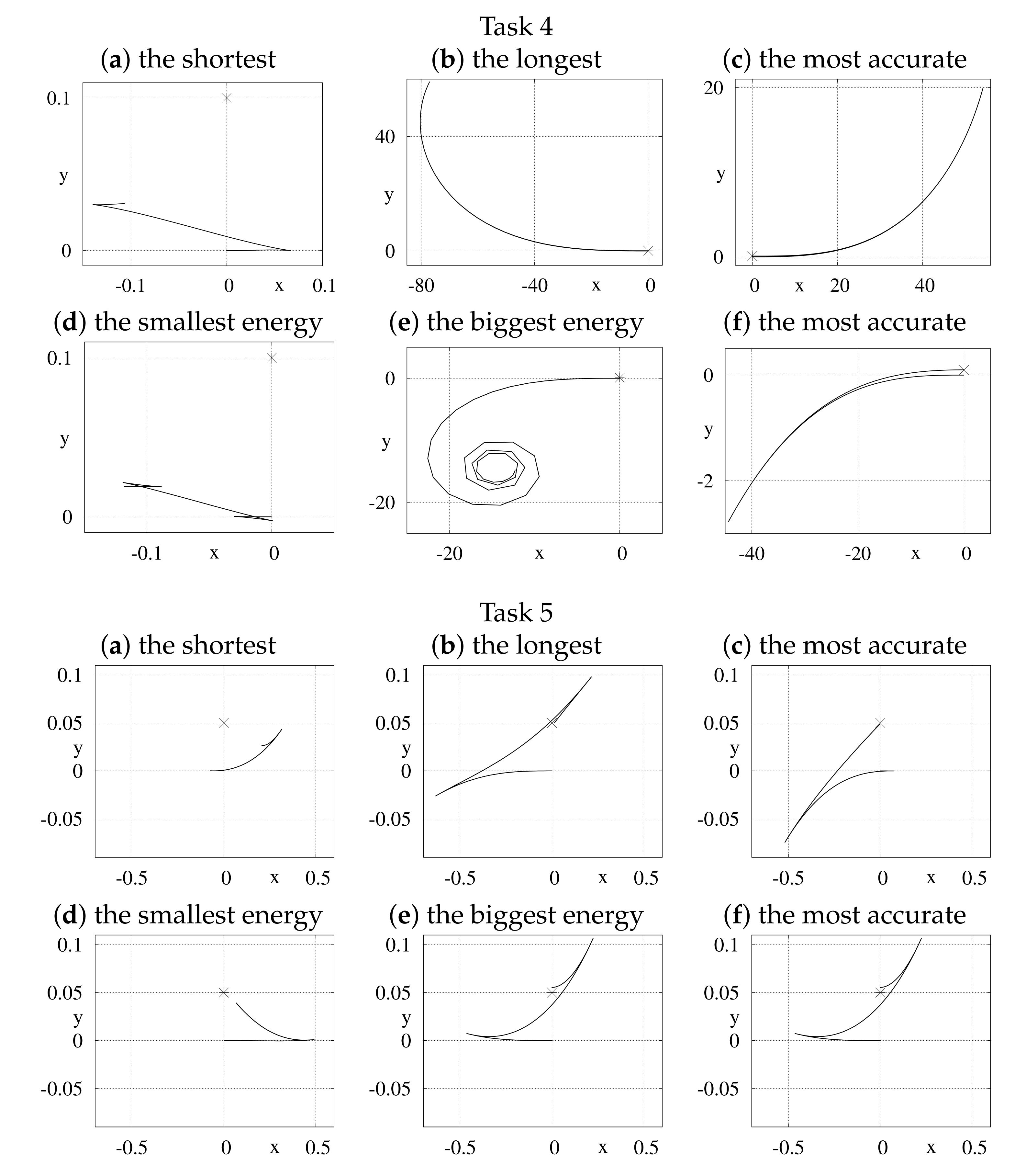
Figure 3.
xy-plane projections of some paths generated with basic (a–c) and null-space optimization (d–f) versions of the Newton algorithm run for the kinematic car.
Some numeric data describing the quality of solutions were collected in Table 2 and Table 3. The abbreviations used:
Table 2.
Accuracy, numeric failures, and computing time for the unicycle tasks.
Table 3.
Accuracy, numeric failures, and computing time for the kinematic car tasks.
- b.a.
- —the best end-point accuracy obtained;
- a.
- —how many generated paths were accurate enough,
- f.
- —the percentage of the Newton algorithm runs which caused numerical problems due to an inversion of near-singularity matrices,
- ctime
- —the average computation time. It is worth noticing that the time includes all stages of running each task, i.e., a symbolic generation of the Ph. Hall basis, kinematic-like mapping, and Jacobians and, finally, a truly numeric trajectory generation.
A path is considered to be accurate if an end-point of generated trajectory in the task-space is close enough to the target point , i.e.,
where —the starting point and — an accuracy coefficient. In Table 2 and Table 3, data were collected for . The most accurate path satisfies
In Table 4 and Table 5, statistical data (length and energy ranges for paths satisfying Condition (26)) were collected. The case when no path meets Condition (26) is marked with a dash (or not included at all when both versions of the Newton algorithm failed).
Table 4.
Path length and energy of motion of the unicycle.
Table 5.
Path length and energy of motion for the kinematic car.
Based on results of the tests, some observations can be formulated:
- Length and energy of resulting paths strongly depend on initial values of , especially when the basic Newton algorithm is used. The Newton algorithm, being local and iterative, has to generate trajectory-dependent results (the next iteration output depends on the output of the current iteration) and it tends to get into a desired location as fast as possible. It may happen that the basic algorithm provides better results than the optimized one. However, a smaller variance of results was observed in the energy-optimized version. In this case, the search space is searched more thoroughly.
- Trajectories generated with the optimized version of the Newton algorithm usually form a few clusters corresponding to local minima. This feature was not observed in the basic algorithm, as trajectories are not constrained by the energy minimization.
- Although the null-space optimization Newton algorithm does not necessarily guarantee the best accuracy, still much more often it promptly reaches the target.
- The failure ratio, cf. Equation (26), is much bigger for non-redundant parameterizations. What is interesting, in some tasks, parameterizations with the same number of parameters, cf. (23) and (24), generate significantly different results. Sometimes a task is solvable in one parameterization, while it is not in the other.
- The optimization within the null space significantly increases computational costs. In order to decrease the costs, this version of the Newton algorithm might be run after the target point was reached using the basic algorithm.
- For the unicycle robot and the identity output function, the quality of the solutions was generally better than that for tasks with smaller dimensional task-spaces, likely due to simplicity of the model and a small number of local minima. However, the length of a path and an energy of motion is smaller for tasks with low-dimensional output functions as it is less restricted.
- Obviously, the higher dimensional output space is, the more difficult task is generated. Additionally, a high redundancy in a parameter space is more computationally costly, but gives more flexibility as well. Thus, a compromise between flexibility and costs has to be found.
- Computational costs are smaller for the identity output function than for other output functions, as there is no need to transfer data between configuration and task spaces.
- Short length steps, characterized by small values of , are easier to control.
- There are a few sources of inaccuracies in motion planning using Lie-algebraic methods: the truncation of the Lie series (5), evaluation of vector fields at although a trajectory surrounds the point (quite well visible for long-range motions) numeric properties of the Newton algorithm. All of them can be controlled by the right choice of parameters.
- A planning accuracy varies substantially with the current configuration , as vector fields in the Lie-algebraic methods are evaluated at the point, cf. Equation (5), and vector fields exhibit different variability around different .
- In almost all xy-projection plots one can notice characteristic cusps, which are typical in Lie-algebraic motion planning. At a close vicinity of a cusp a tangent line to the trajectory remains almost the same, while direction of motion is changed. It means that due to particular values of controls and generators, some components of velocity in Equation (1) change their signs while passing through zero. An illustrative example of such behavior can be constructed by setting: long, short, small, and control passing though zero. Therefore, one can expect that the number of cusps strongly and positively correlates with frequencies of controls. For mobile robots tested the explanation is even simpler, as the cusps result from linear velocity sign changes.
- Many trajectory cusps result in a zigzag motion, which is especially useful in obstacle-cluttered environments as the volume of maneuvers can be controlled and kept small. However, it is also visible that generating a relatively short motion along high degree vector fields requires a relatively long path to follow.
- Results for the kinematic car are the most interesting, especially for the identity output function. In this case, a hard to meet condition forces extensive movement. This condition is particularly difficult to satisfy for non-redundant parameterizations. Therefore, in some sub-figures of Task 4, cf. Figure 3, scales of axes were extended to present the whole paths. Nevertheless, the point (cf. Figure 3 b,c,e,f) is close to the desired point as required.
- It may look strange that in Task 6, cf. Figure 3e, the projected path with the biggest energy is relatively short. In this case, the major contribution to the energy consumption was caused by control , responsible for reorientation of the robot.
4. Conclusions
In this paper, the Lie-algebraic method of motion planning for nonholonomic systems, originally designed to plan within the configuration space, has been extended to also work in a task-space. There are some advantages of planning within the task-space:
- a smaller than the configuration space dimension either increases redundancy and facilitates optimizing a motion or allows to decrease the number of parameters of controls,
- it allows to define and solve many practical tasks, especially in obstacle-cluttered environments when some components of the configuration vector are not important.
However, there are also some disadvantages:
- a new source of singularities introduced by the output mapping,
- the impossibility to plan only within the task-space, without referring explicitly to the configuration space (usually the task-space dimension is smaller than the configuration space dimension, thus no unique mapping between the two spaces exists).
Some general observations based on simulation results:
- Depending on the planning purpose, the Newton algorithm, extensively used in the proposed algorithm, can be applied with or without optimization. The first version (low computational costs) should be used for tasks with no extra requirements or as a first try solution.
- A small redundancy in setting the search space size () is advised not to cause a significant increase of computational costs, while preserving flexibility and solvability of planning tasks.
- An initial value of the parameter vector highly impacts solvability of the planning task and also the resulting trajectory shape. Therefore, the multi-start technique is recommended, especially when planning is performed in the off-line mode.
Our future research will concentrate on applications of the Lie-algebraic method in difficult environments (narrow passages, non-convex obstacles) in the task-space. In such environments, the planning should be performed through selection of sub-goals on the way to the target position. The main difficulty is the sub-goal selection is caused by the fact that nonholonomic systems are not governed by the Euclidean geometry, but rather the sub-Riemannian one [19]. The Lie-algebraic method is local and general-purpose, thus it is particularly well suited for solving tasks in partially known or dynamic environments.
Author Contributions
Conceptualization, A.M. and I.D.; methodology, A.M. and I.D.; software, A.M.; validation, A.M. and I.D.; formal analysis, A.M. and I.D.; resources, A.M. and I.D.; writing—original draft preparation, I.D.; writing—review and editing, I.D.; visualization, A.M. All authors have read and agreed to the published version of the manuscript.
Funding
This research was funded by the Wroclaw University of Science and Technology within Grant No. 821 110 41 60.
Conflicts of Interest
The authors declare no conflict of interest.
References
- Duleba, I. Kinematic models of doubly generalized N-trailer systems. J. Intell. Robot. Syst. 2019, 94, 135–142. [Google Scholar] [CrossRef] [Green Version]
- Vafa, Z.; Dubowsky, S. The kinematics and dynamics of space manipulators: The virtual manipulator approach. Int. J. Robot. Res. 1990, 9, 3–21. [Google Scholar] [CrossRef]
- Dubins, L.E. On curves of minimal length with a constraint on average curvature, and with prescribed initial and terminal positions and tangents. Am. J. Math. 1957, 79, 497–516. [Google Scholar] [CrossRef]
- Reeds, J.A.; Shepp, L.A. Optimal paths for a car that goes both forwards and backwards. Pac. J. Math. 1990, 145, 367–393. [Google Scholar] [CrossRef] [Green Version]
- Murray, R.M.; Sastry, S.S. Nonholonomic Motion Planning: Steering Using Sinusoids. IEEE Trans. Autom. Control 1993, 38, 201–215. [Google Scholar] [CrossRef] [Green Version]
- Dulęba, I.; Sąsiadek, J. Nonholonomic motion planning based on Newton algorithm with energy optimization. IEEE Trans. Control. Syst. Technol. 2003, 11, 355–363. [Google Scholar] [CrossRef]
- Tchoń, K.; Jakubiak, J. Endogenous configuration space approach to mobile manipulators: A derivation and performance assessment of Jacobian inverse kinematics algorithms. Int. J. Control 2003, 26, 1387–1419. [Google Scholar] [CrossRef]
- Duleba, I.; Wissem Khefifi, W.; Karcz-Duleba, I. Layer, Lie algebraic method of motion planning for nonholonomic systems. J. Frankl. Inst. 2012, 349, 201–215. [Google Scholar] [CrossRef]
- Jakubczyk, B. Nonholonomic path following with fastly oscillating Controls. In Proceedings of the 9th Workshop on Robot Motion and Control, Wąsowo, Poland, 3–5 July 2013; pp. 99–103. [Google Scholar]
- Arismendi, C.; Alvarez, D.; Garrido, S.; Moreno, L. Nonholonomic Motion Planning Using the Fast Marching Square Method. Int. J. Adv. Robot. Syst. 2015, 12, 1–14. [Google Scholar] [CrossRef]
- Gawron, T.; Michałek, M.M. The VFO-driven motion planning and feedback control in polygonal worlds for a unicycle with bounded curvature of motion. J. Intell. Robot. Syst. 2018, 89, 265–297. [Google Scholar] [CrossRef]
- Łakomy, K.; Michałek, M.M. Robust output-feedback VFO-ADR control of underactuated spatial vehicles in the task of following non-parametrized paths. Eur. J. Control 2021, 58, 258–277. [Google Scholar] [CrossRef]
- LaValle, S. Planning Algorithms; Cambridge University Press: Cambridge, UK, 2006. [Google Scholar]
- Lynch, K.M.; Park, F.C. Modern Robotics: Mechanics, Planning, Control; Cambridge University Press: Cambridge, UK, 2017. [Google Scholar]
- Chow, W.L. Über Systeme von linearen partiellen Differentialgleichungen erster Ordnung. Math. Ann. 1939, 117, 98–105. [Google Scholar]
- Strichartz, R.S. The Campbell-Baker-Hausdorff-Dynkin Formula and Solutions of Differential Equations. J. Funct. Anal. 1987, 72, 320–345. [Google Scholar] [CrossRef] [Green Version]
- Duleba, I.; Khefifi, W. Pre-control from of the gCBHD formula and its application to nonholonomic motion planning. In Proceedings of the IFAC Symposium on Robot Control, Wroclaw, Poland, 1–3 September 2003; Dulęba, I., Sąsiadek, J.Z., Eds.; Elsevier: Oxford, UK, 2004; Volume 1, pp. 123–128. [Google Scholar]
- Nakamura, Y. Advanced Robotics: Redundancy and Optimization; Addison-Wesley: Boston, MA, USA, 1991. [Google Scholar]
- Agrachev, A.; Barilari, D.; Boscain, U. A Comprehensive Introduction to Sub-Riemannian Geometry; Cambridge University Press: Cambridge, UK, 2019. [Google Scholar]

Publisher’s Note: MDPI stays neutral with regard to jurisdictional claims in published maps and institutional affiliations. |
© 2021 by the authors. Licensee MDPI, Basel, Switzerland. This article is an open access article distributed under the terms and conditions of the Creative Commons Attribution (CC BY) license (https://creativecommons.org/licenses/by/4.0/).