1. Introduction
The intersection between combinatorial optimization and Hyper-Heuristics (HHs) is a relevant and active area in literature, as Sánchez et al. detailed with their thorough systematic review [
1]. The former considers optimization problems where a permutation of feasible values gives candidate solutions. The hardness of these problems could be easy or hard to solve, depending on different parameters. Among them resides a category known as NP-hard problems, for which analytical solvers cannot be scaled due to an excessive computational burden. Therefore, approximate solvers are commonly sought for NP-hard problems, including those based on heuristics. It is here where HHs shine bright. This approach has been deemed as high-level heuristics useful to tackle hard-to-solve problems [
2], particularly NP-hard ones [
3]. A classification of HHs considers two main groups: selection HHs (those that select heuristics from an available set) and generation HHs (those that create new heuristics using components of existing ones) [
4]. Although both groups have proved of great interest to the scientific community, in this work we focus on the former.
Selection HHs deal with problems indirectly. They browse a set of available heuristics, which are selectively applied to solve the problem at hand [
5]. A selection HH analyzes a set of available heuristics and chooses the most suitable one according to a given performance metric. Most of the current selection HH models include two key phases: heuristic selection and move acceptance [
6]. The former represents the strategy for deciding which heuristic should be selected. Conversely, the latter determines whether the new solution is accepted or discarded. The approach proposed in this work simplifies the overall model by only focusing on heuristic selection. Thus, changes resulting from applying a particular heuristic are always accepted.
Evolutionary computation is a recurrent approach among the many learning methods employed in the literature to produce HHs. Some examples include, but are not limited to, Genetic Programming (GP) [
5,
7,
8,
9], Grammatical Evolution (GE) [
10], Genetic Algorithms (GA) [
11,
12], and Artificial Immune Systems (AIS) [
13,
14]. The literature contains other related proposals, such as those that evolve HHs by analyzing the set of problem instances [
15]. These findings support the idea of using an evolutionary strategy as a learning mechanism for HHs, one which improves their performance via crossover or mutation. This work focuses on the latter.
HHs have been used to tackle packing problems in the past. Hart and Sim describe a variant of AIS used as a hybrid HH for the Bin Packing Problem [
13,
14,
16]. Falkenauer [
11] proposed a GA-based HH model, and Burke et al. [
17], Hyde [
8], and Drake et al. [
9,
18,
19] have studied GP rules for the Bin Packing and Multidimensional Knapsack problems. More recent studies of HHs have been conducted on the binary knapsack domain using Ant Colony Optimization [
20] and Quartile-related Information [
21]. Further information about the state-of-the-art of HHs and their applications are provided in [
4,
22].
As mentioned above, several combinatorial optimization problems have been tackled with HHs [
1]. This paper focuses on the Knapsack Problem (KP), which has been studied in great depth due to its simple structure and broad applicability. Example applications include cargo loading, cutting stock, allocation, and cryptography [
23]. When a constructive approach is used to solve this problem, the solution is built one step at a time by deciding if one particular item must be packed or ignored. For simplicity, our setting states that once the process chooses an item, there is no way to change such a decision. Using a constructive approach leads to different subproblems throughout the solving process, depending on the heuristic used. This happens because packing an item produces an instance with a reduced knapsack capacity (the previous knapsack capacity minus the weight of the packed item) and a reduced list of items (the item recently packed or ignored is no longer part of the items to pack). This behavior raises the question of which heuristic, among the different options, should be used to maximize the overall profit resulting from the items contained in the knapsack. The literature usually refers to the problem of selecting the best algorithm for a particular situation as the Algorithm Selection Problem [
24].
Despite the extensive use of selection HHs [
4,
25], only a few works explore the insights of their behavior. A few examples include a run-time analysis [
26,
27], the use and control of crossover operators [
19], and heuristic interaction when applied to constraint satisfaction problems [
28]. Furthermore, traditional selection HH models, that represent the relation between problem states and heuristics through 〈condition, action〉 rules, exhibit a significant limitation: they require the definition of a set of features to characterize the problem state [
29]. Finding such a set of features implies an additional layer of complexity to the model. To the best of our knowledge, there is only one work on feature-independent HHs for the knapsack problem, which obtained only a few preliminary results [
30]. Therefore, our work aims at filling this knowledge gap through two particular contributions:
It proposes an evolutionary-powered hyper-heuristic framework capable of combining the strengths of individual heuristics when solving sets of KP instances.
Besides the model itself, it provides the analysis and understanding of the performance of the hyper-heuristics designed under this model on instance sets formed by challenging instances, both balanced and unbalanced (in terms of heuristic performance).
The remainder of this document is organized as follows.
Section 2 defines the fundamental ideas associated with our work.
Section 3 describes the HH model and the rationale behind it.
Section 4 details the experiments conducted and analyzes the results. Finally,
Section 5 presents the conclusions and provides an overview of future directions for this investigation.
3. Proposed Hyper-Heuristic Model
The HH model developed in this work can be classified as an offline selection HH [
56]. Internally, the HH model relies on a variant of the
Evolutionary Algorithm (EA) to find the sequence of heuristics to apply. The original EA flipped each bit with probability
(where
is the chromosome length). Conversely, our approach chooses one among various available mutation operators based on a uniform random probability distribution. This EA implementation considers some of the features used by Lehre and Özcan [
27]. However, the set of available operators is different as we work with constructive heuristics while they have used perturbative ones.
We choose four simple packing heuristics due to their popularity: {Def, MaxP, MaxPW, MinW}. Before moving forward, we describe them below.
- Default
(Def) packs the items in the same order that they are contained in the instance, as long as they fit in the knapsack.
- Maximum profit
(MaxP) sorts the items in descending order based on their profit and packs them in that order as long as they fit in the knapsack.
- Maximum profit per weight
(MaxPW) calculates profit-over-weight ratio for each item and sorts them in descending order. Then, MaxPW follows this ordering until the knapsack is full or no more items are left to be packed.
- Minimum weight
(MinW) favors lighter items, so it sorts items in ascending order based on their weight and packs them by following such order until they no longer fit.
Should there be a tie, all heuristics will choose the first conflicting item. Among these heuristics, Def is the fastest one to execute as it involves no additional operations. On the contrary, MaxP, MaxPW, and MinW take longer to compute but usually yield better results than using no order at all (Def). We are aware that more complex heuristics are available in the literature. Still, at this point in the investigation, we consider it suitable to test the proposed HH approach on this set of simple heuristics.
In our model, each HH represents a sequence of heuristics to apply to the problem in one specific order. For simplicity, we refer to its length as the cardinality of the HH. Let us consider the HH with cardinality of five (
) given by
{
Def,
MaxP,
MaxP,
Def,
MinW} (
Figure 1). Please note that one of the available heuristics is not contained within the HH,
MaxPW. In this HH,
Def occupies positions 0 and 3,
MaxP occupies positions 1 and 2, and
MinW occupies position 4. Let us assume that
will solve a 12-item knapsack instance. In this case, there are 12 decisions to be made for solving this instance (
to
). While some of the decisions will add an item to the knapsack, others will discard it. As the HH represents a sequence of five heuristics, the first five decisions will be made in the same order in which the heuristics are presented in
:
Def,
MaxP,
MaxP,
Def, and
MinW. After that, there are no more heuristics to choose to make further decisions. Then, the HH is used again, but now backwards:
MinW,
Def,
MaxP,
MaxP, and
Def. The process repeats by inverting the sequence every time we reach the end of the HH. Although this scheme seems disruptive, we consider it feasible to favor the changes in heuristics throughout the solving process.
3.1. Hyper-Heuristic Training
The learning mechanism within the HH model works as follows. The HH,
, is randomly initialized (with a sequence of
randomly selected heuristics), and it is used to solve the set of training instances. We register the profit of the solution obtained by
for each instance. The performance of the HH,
, is then calculated as the average of all the profits obtained for the training set. In our EA implementation, a chromosome represents a HH that codes a sequence of heuristics to apply, i.e.,
. At each iteration, the process randomly chooses one mutation operator
from the available operators
. To do so, a uniform probability distribution is employed. Thus, EA applies it on a copy of the current HH, which produces a candidate HH, according to (
2). The model evaluates the candidate HH on the set of training instances. If its performance is greater or equal (to favor diversity) than the current HH, this candidate takes its place. The process is repeated until it reaches the maximum number of allowed iterations
. Pseudocode 1 details this training procedure.
The main goal of the learning mechanism is to produce a HH (an ordered sequence of heuristics) that maximizes the profit of an instance by packing appropriate items into the knapsack. In other words, it solves (
1). Thus, the EA does not operate on the solution space
, but on the heuristic space
.
| Pseudocode 1 Hyper-heuristic trainer |
input: Set of heuristics , Set of mutation operators , Set of instances to train the hyper-heuristic , Initial cardinality , Performance function , and Maximum number of iterations output: Best selection hyper-heuristic
- 1:
InitializeRandomly(, ) - 2:
, ▹ Evaluate the current HH - 3:
for i = 0 to do - 4:
GenerateCandidate() - 5:
, ▹ Evaluate the candidate HH - 6:
if then - 7:
and - 8:
end if - 9:
end for - 10:
return -
- 11:
procedure GenerateCandidate() - 12:
Clone() - 13:
←ChooseRandomly() - 14:
▹ Mutate by applying - 15:
return - 16:
end procedure
|
3.2. Mutation Operators
The evolutionary process dynamically chooses among eight available mutation operators to alter the candidate hyper-heuristic
. Operators contained within set
are described below. To clarify the behavior of such operators, we also provide a brief example of their behavior. Bear in mind that, in all the examples, we always consider the HH depicted in
Figure 1 as the HH to mutate, i.e.,
= {
Def,
MaxP,
MaxP,
Def,
MinW}.
- Add
inserts a randomly chosen heuristic at a random position into . In doing so, cardinality () increases by one and existing heuristics at this position onward are shifted to the right. For the example, let us assume that and that the random selection chooses MaxPW. Thus, the resulting HH has a cardinality of six and is given by {Def, MaxP, MaxP, MaxPW, Def, MinW}.
- Single-point Flip
selects a position at random from and changes its heuristic to a different one (selected at random). Thus, cardinality is preserved. Let us suppose that . As Def is the current heuristic at this position, it cannot be chosen. Therefore, let us assume that the new heuristic is MinW. Then, the resulting HH is {MinW, MaxP, MaxP, Def, MinW}.
- Two-point Flip
is a more disruptive version of the previous operator. This time, heuristics at two different positions () are renewed. Let us suppose that and . In the first case, the available heuristics are Def, MaxPW, and MinW. In the second one, they are Def, MaxP, and MaxPW. Imagine that MaxPW and Def are selected, respectively. Then, the resulting HH still preserves cardinality and is given by = {Def, MaxP, MaxPW, Def, Def}.
- Neighbor-based Add
is similar to Add as it also inserts a heuristic at a random position within . However, the heuristic to insert is randomly selected among neighboring heuristics (positions and ), as long as they are valid positions. Should i correspond to an edge, the only neighbor is copied. Let us suppose that . In this case, the heuristic to insert would be either Def () or MaxP (), with the same probability (50%). Imagine that MaxP is selected. Then, and as with the Add operator, cardinality grows to six and the resulting HH is = {Def, MaxP, MaxP, MaxP, Def, MinW}.
- Neighbor-based Single-point Flip
is a variant of Single-Point Flip where the heuristic at changes into one of its neighbors (positions and , if they exist). For example, suppose that . In this case, candidate replacements would be either MaxP () or Def (), each one with a 50% probability. Let us suppose that Def is selected. Then, the resulting HH preserves cardinality and becomes = {Def, MaxP, Def, Def, MinW}.
- Neighbor-based Two-point Flip
likewise, this is a variant of Two-Point Flip in which heuristics are chosen at random from neighboring ones. Let us suppose that and . In the first case, available heuristics are MaxP and Def; in the second one, it is only Def since the position corresponds to an edge of the HH. Let us suppose that, in the first case, Def is selected. Therefore, the resulting HH is = {Def, MaxP, Def, Def, Def}.
- Swap
interchanges heuristics at two randomly selected locations, , and so preserves cardinality. For example, assume that and . Thus, the resulting HH becomes = {Def, Def, MaxP, MaxP, MinW}.
- Remove
randomly selects one position within the HH and removes the heuristic at that position. Therefore, cardinality is reduced by one. After removing the heuristic, upcoming ones are shifted to the left. For example, imagine that . Then, the resulting HH has a cardinality of four and is given by: = {MaxP, MaxP, Def, MinW}.
Note that neighbor-based operators are allowed to replace the corresponding heuristic with the same one since it is determined by the neighbors. Certainly, other operators can be used but, for the sake of simplicity, we limit ourselves to these eight to formulate . Finally, consider that there is only one operator that reduces cardinality (Remove), while two of them increase it (Add and Neighbor-based Add), and the remaining five preserve it (Single-point Flip, Two-point Flip, Single-point Neighbor-based Flip, Two-point Neighbor-based Flip, and Swap). Therefore, it is rather expected that trained HHs exhibit a higher cardinality than untrained ones. Because of this, a HH may end up choosing a different amount of items with each heuristic. We believe such flexibility in the learning process may favor more complex interactions between the available heuristics.
3.3. The Knapsack Problem Instances
In this investigation, we consider four datasets:
,
,
, and
. Dataset
is used for training purposes and comprises 400 knapsack problem instances. We synthetically generated such instances for this work by using the algorithm proposed by Plata et al. [
57]. This dataset contains a balanced mixture of problem instances, where each heuristic has an equal probability of performing best. Therefore, we are sure that no single heuristic outperforms others on all instances. We replicated the process to produce 400 additional problem instances for testing purposes (dataset
). These two datasets consider instances of 50 items and a knapsack capacity of 20 units. Dataset
contains 600 hard instances proposed by Pisinger [
45] and featuring 20 items but at different capacities. Finally, dataset
consists of 600 additional hard instances (also proposed by Pisinger [
45]). In this case, instances have 50 items and, again, exhibit different capacities. A summary of the datasets is provided in
Table 1. Bear in mind that for the confirmatory experiments, we analyze the effect of changing the training dataset, but we shall discuss it in more detail further on.
3.4. Performance Metrics
We evaluate performance by considering both absolute and relative performances. All approaches are evaluated based on the profits obtained by their solutions (the sum of the profits of the items packed within the knapsack). The overall performance of a method on a particular set is calculated as the sum of the profits of the solutions produced for all the instances in such a set. However, it is also useful to estimate the relative performance, i.e., w.r.t. the other methods. For this purpose, we also include a performance ranking and the success rate ().
The performance ranking is calculated as follows. All methods solve every instance in the set. Then, for each instance, the methods are sorted based on the profit of their solutions. The best one receives a ranking of 1, the second one a ranking of 2, and so on. In the case of ties, the ranking is the average of tied positions. This metric is helpful to identify ties that indicate a similar performance of two or more methods. Conversely, the success rate is calculated as the percentage of instances in a set where a particular method reaches or surpasses a threshold. In this investigation, such a threshold is given per instance and corresponds to the best result among those achieved by the heuristics, i.e., the best profit we can get from using each heuristic individually. For the sake of clarity, we present the success rate as a vector of two components: one where the threshold is achieved and one where it is surpassed. Bear in mind that the second component in the vector can only be achieved by mixing heuristics throughout the solving process, and so it only applies to HHs.
4. Experiments and Results
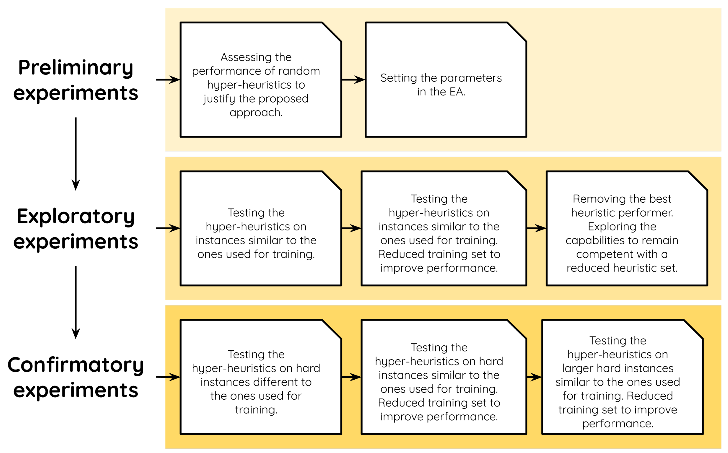
We organized our experiments in three stages: preliminary, exploratory, and confirmatory experiments. For the sake of clarity, these stages are further divided into categories.
Figure 2 provides an overview of our experimental methodology. In the following lines, we carefully describe each stage, the corresponding experiments, and the results we obtained.
4.1. Preliminary Experiments
The preliminary experiments were designed first to justify the need for an intelligent way to combine the heuristics (the HHs) and, second, to determine a suitable set of parameters for running the EA to produce such HHs.
4.1.1. Preliminary Experiment I
The first experiment conducted in this work aims to prove that we need an intelligent approach to define the sequences of heuristics. In other words, we justify that it is unlikely for a random sequence of heuristics to achieve competent results. For this purpose, we generated 30 random HHs. The length of these HHs was set to 16 heuristics for empirical reasons. As in this experiment, we were only interested in the behavior of randomly generated HHs, the EA was not used to improve the initial HHs. Then, we used the 30 randomly generated HHs to solve set
, and we compared their results against the ones obtained by the available heuristics (see
Section 3 for more details). For the sake of clarity, our comparisons include the results of three representative HHs from the perspective of total profit on set
: the best, the median, and the worst hyper-heuristics.
One way to analyze the performance of the methods relies on ranking the resulting data.
Table 2 shows the ranks obtained by the four heuristics, as well as the three representative HHs, when solving set
. As one may observe, in most of the cases, the heuristics obtain the best result in isolation (ranks close to 1), as it was expected as set
is balanced. Although the best HH never occupies the last positions in the rank, the median performance hints that the good behavior of
Best-HH is more likely to be due to chance. Furthermore, by randomly generating the sequences of heuristics, we risk producing something as bad as
Worst-HH, where it replicated the worst heuristic for this set, i.e.,
Def.
Table 2 also shows the total profit obtained for each method on set
, which serves as evidence that it is indeed possible to produce one good HH at random, such that it outperforms several heuristics. However, this seems unlikely to happen by chance since at least half the HHs perform worse than
MinW.
Regarding the success rate, the results confirm that generating sequences of heuristics at random is not a good idea. The success rate of the best randomly generated HH was , which means that only in 5% of the instances in set this HH produced a solution as competent as the best one among the four heuristics, while in 0.25% of the instances for the same set, the HH improved upon this result.
4.1.2. Preliminary Experiment II
Before moving further in this investigation, we needed to fix the number of iterations for the EA. Therefore, we generated 30 HHs by running the EA for 1000 iterations each time. In all the cases, the initial HH contained sequences of 12 heuristics, and we used
as the training set. This time, the cardinality of the HHs was reduced by
concerning the previous experiment since the mutation operators allow shortening and extending the sequences. Then, we no longer need long initial sequences as with the first preliminary experiment. For each HH, we recorded the Stagnation Point (SP). We define SP as the iteration at which the best solution was first encountered and for which the profit showed no improvement in subsequent iterations.
Table 3 shows the stagnation points of the 30 runs of the EA.
We used these stagnation points to estimate the maximum number of iterations for running the EA. The average stagnation point among the 30 runs was 150.1, so we rounded it down to 150 iterations. Fifty additional iterations were added just as a precaution to minimize the risk of not reaching a good result. Thus, we set the maximum number of iterations to 200 for the rest of the experiments.
4.2. Exploratory Experiments
The exploratory experiments comprise a series of tests that cover general aspects of the proposed model, particularly those regarding how it copes with single heuristics on the balanced instance sets (sets and ).
4.2.1. Exploratory Experiment I
In this experiment, the rationale was to test the performance of HHs on similar instances to those they were trained on. Therefore, we produced 30 HHs with an initial cardinality of 12 heuristics each, as in preliminary experiment 2 (
Section 4.1.2). Each HH was trained using set
for 200 iterations. Afterward, we tested the resulting HHs on set
and we compared the data against those obtained by heuristics applied in isolation.
Table 4 presents the ranking of the four heuristics as well as the best, median, and worst HHs produced in this experiment and tested on set
. This table also shows the total profit obtained by each of these methods on the same set. Based on the results obtained (both on ranks and total profit), we observe that the process is forcing the HHs to replicate the behavior of the best performing heuristic for these types of instances (
MaxPW). This also means that the HHs are, most of the time, ignoring the remaining heuristics. Although this may seem like a good choice as
MaxPW is the best individual performer, the HHs are sacrificing the opportunity to improve their overall performance and outperform the best individual heuristic.
4.2.2. Exploratory Experiment 2
In the previous experiment, the EA forced the HHs into replicating the behavior of one heuristic,
MaxPW. In this experiment, we try to overcome this situation by reducing the number of instances in the training set. Then, for this experiment, 30 new HHs were produced, but this time, only 60% of the instances in set
were used for training purposes. These 60% instances were randomly selected once and used for producing the 30 HHs. As in the previous experiment, the maximum number of iterations for the EA was set to 200 and all the HHs were initialized by using a random sequence of 12 heuristics. We used the 30 HHs to solve set
and summarized the results through the rankings and total profit (
Table 5).
Based on the results shown in
Table 5, we observe a small improvement in
Best-HH with respect to
MaxPW. Although this supports our initial idea that we can improve the results obtained by the heuristics with a hyper-heuristic, the improvement is rather small and insignificant in practice. Furthermore, the success rate of
Best-HH is
, which is exactly the same as
MaxPW.
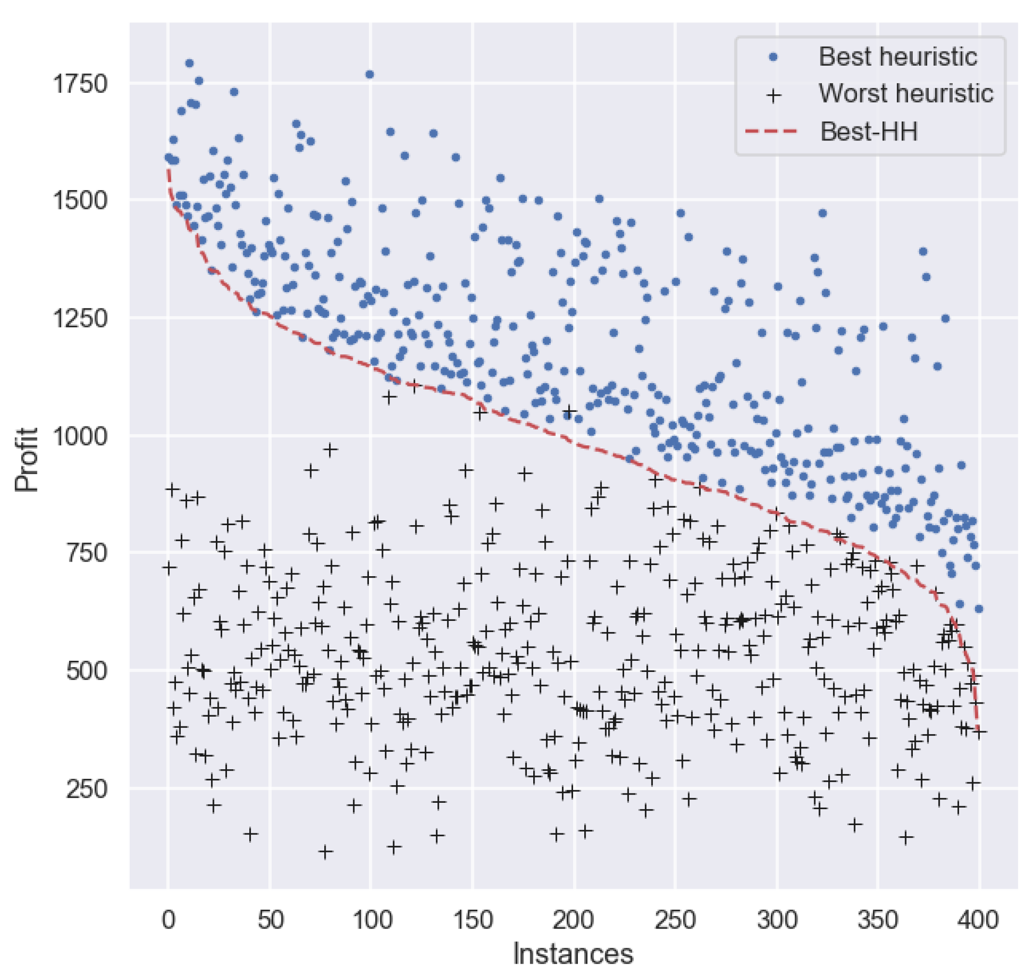
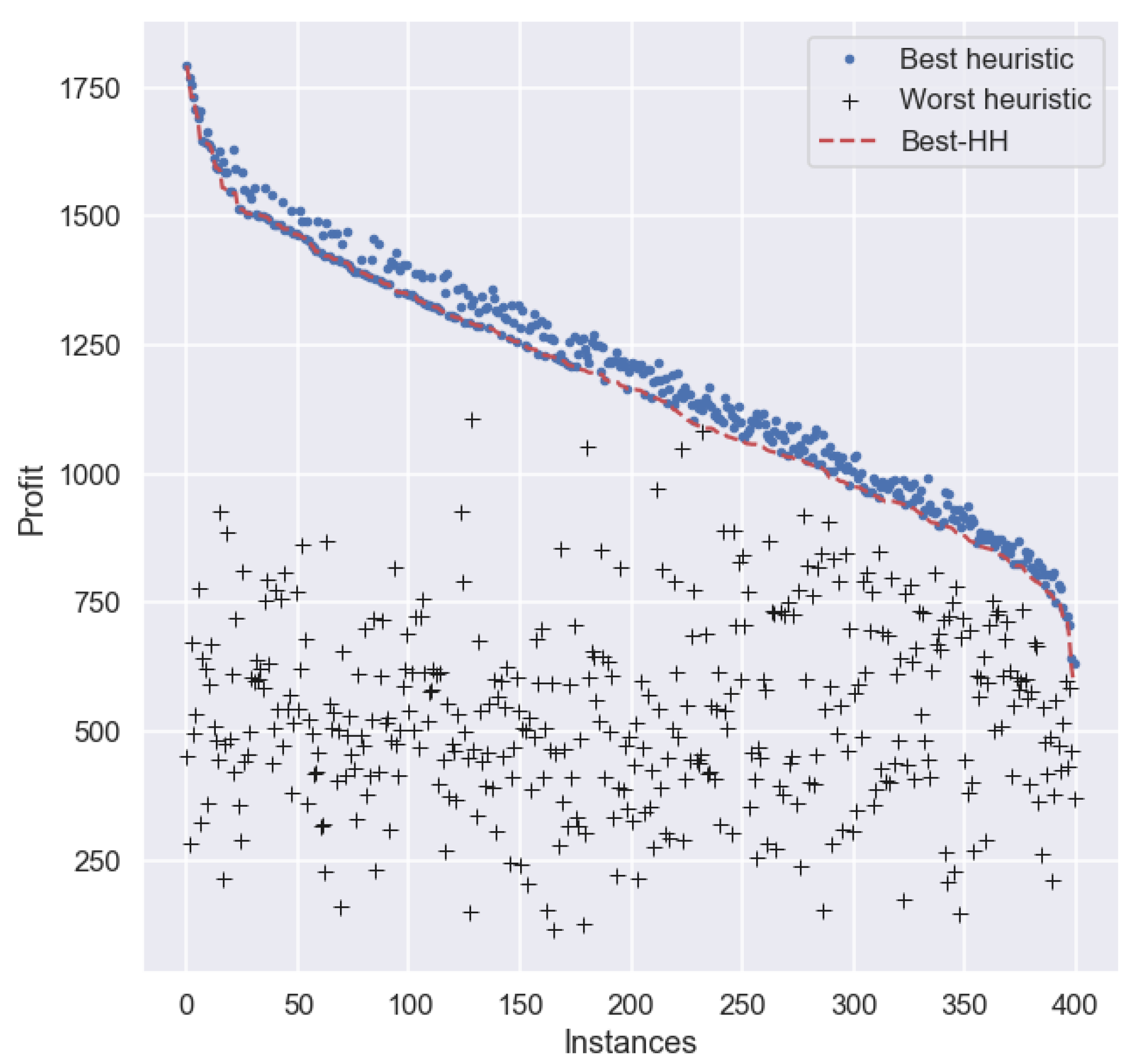
For a more in-depth analysis about the performance of the best HH in this experiment, we plotted the performance of
Best-HH, as well as of the best and worst heuristic for each particular instance in set
. For clarity, the results are sorted (from larger to smaller) on the profit obtained by
Best-HH on each instance in the set.
Figure 3 depicts the profit of each method across all instances. As we can observe, there are many cases where
Best-HH obtains a smaller profit than the best heuristic for each particular instance.
4.2.3. Exploratory Experiment III
So far, we have observed that, even though it is possible to overcome the best individual performer for each instance in some specific cases, oftentimes the HHs tend to replicate the behavior of the overall best heuristic (MaxPW for sets and ). Although this is not a bad result—the model produces very competent HHs, it is difficult to justify the additional time devoted to producing such HHs given the small gains with respect to MaxPW. For this reason, in this experiment we wanted to explore the case where the HHs can only choose among Def, MaxP, and MinW (all the available heuristics but MaxPW) and evaluate if the HHs produced may still be considered competent. As in the previous experiments, we generated 30 HHs by training on set for 200 iterations each, and testing on set . In all the cases, the HHs have an initial cardinality of 12 heuristics.
A comparison between the total profits of
Best-HH and
MaxPW (
Table 6) reveals that a significant efficiency was lost due to the removal of
MaxPW from the pool of heuristics (
Figure 4). However, all three representative HHs (best, median, and worst) obtained the second rank in terms of total profit. The profit of
Best-HH shows an improvement of nearly 6% and over 64% with respect to the
MinW and
Def heuristics, respectively. Therefore, the model can learn in harsh conditions and thus obtains promising results regardless of whether it was given a pool of heuristics with limited quality.
4.3. Confirmatory Experiments
Seeking to test the generalization properties of the proposed HH model, we conducted three additional experiments that now incorporate problem instances taken from the literature. These experiments were conducted in a similar way to the exploratory ones: each one involves the generation of 30 HHs with an initial cardinality of 12, which were trained for 200 iterations. However, this time we tried some combinations of the instance sets for training and testing. The rationale behind these experiments is to observe how well the HHs adapt to changes in the properties of the instances being solved with respect to the instances used for producing such HHs.
4.3.1. Confirmatory Experiment I
So far, we have evaluated the performance of HHs on instances similar to the ones used for training, under various scenarios. In the first confirmatory experiment, we use all the instances from set
to train the HHs, but test their performance on set
. Let us recall that set
contains 600 hard instances proposed by Pisinger [
45] and feature 20 items and different capacities. The relevant issue regarding set
is that such instances are considered hard to solve.
Table 7 shows that
MaxPW is, once again, the best individual performer in this experiment. Although all the produced HHs perform similarly (cf.
Worst-HH), they are unable to improve upon the results obtained by the best heuristic. Nonetheless, all the HHs produced obtained a total profit larger than those obtained by the remaining heuristics.
Even if the HHs were incapable of overcoming MaxPW in this experiment, it is interesting to see how close their performance is, especially as these HHs were trained with instances of a different type than those used for testing.
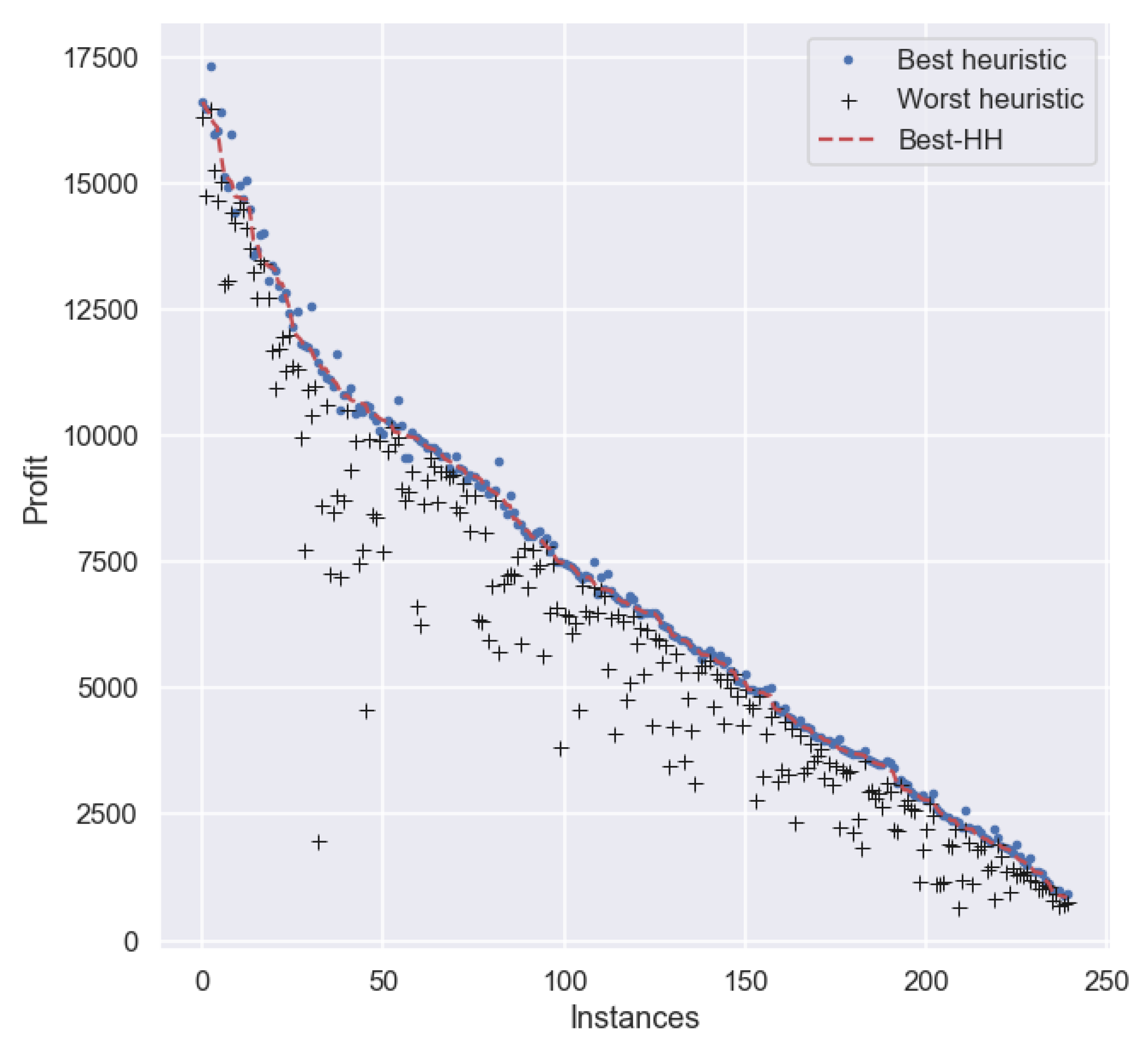
4.3.2. Confirmatory Experiment II
In the previous experiment, we evaluated the performance of HHs trained on balanced sets of instances when tested on hard instances, and we observed a limited capacity to deal with such instances. In this experiment, we show that this behaviour is not due to the hardness of the instances, but because of the discrepancy between the instances used for training and the ones used for testing. For this reason, this experiment is twofold: (1) we test how HHs behave when trained and tested on hard instances (set
) and (2) we try to reduce the effect of
MaxPW in the resulting HHs by reducing the number of instances in the training set. Then, we produced 30 new HHs using only 60% of the instances in set
for training purposes. As in previous experiments, the 60% instances were randomly selected once and used for producing the 30 HHs. For consistency, the maximum number of iterations for the EA was set to 200 and all the HHs were initialized to a cardinality of 12. The HHs produced in this experiment were evaluated on the remaining 40% of the instances in set
. The results for rankings and total profit derived from this experiment are summarized in
Table 8.
This experiment confirms the importance of the instances used for training and their similarity with those solved during the test process. This time, the performance of most of the hyper-heuristics produced using 60% of set
when tested on the remaining 40% of set
improve on
MaxPW (the best heuristic for this set). In fact, the performance of
Worst-HH is practically the same as
MaxPW (
Figure 5). Although the results suggest that an improvement in the total profit can be obtained by using the proposed hyper-heuristic approach, the gain in profit derived from using
Best-HH instead of
MaxPW is rather small (<0.5%). However, this result should not be interpreted as an indication that
Best-HH is replicating the behavior of
MaxPW. In fact, their overall profit is similar (with a small gain for
Best-HH but their specific performance is not. As depicted in
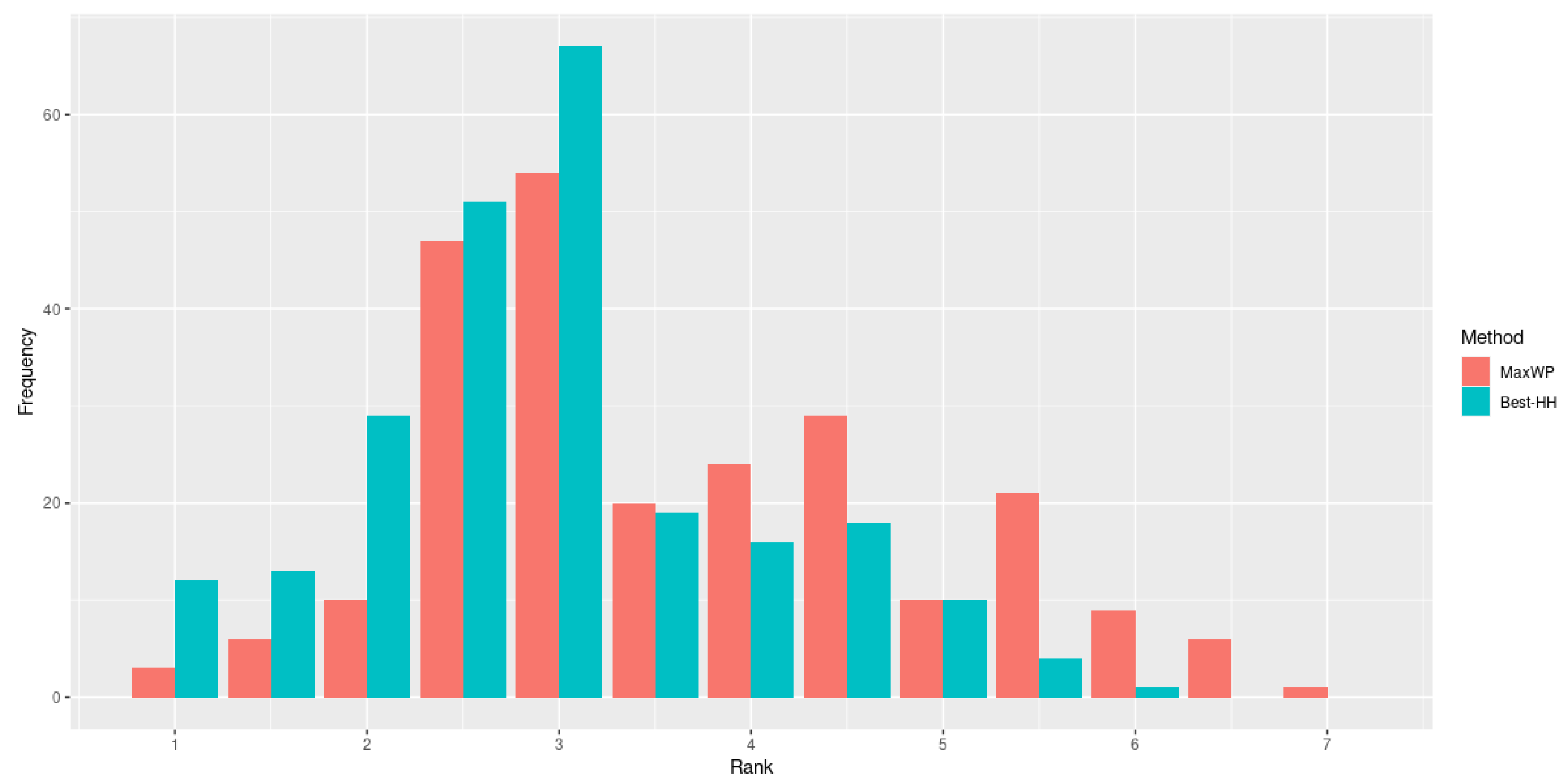
Figure 6, when the ranks are analyzed, we observe that
Best-HH obtains better results in more cases than the best individual heuristic,
MaxPW.
4.3.3. Confirmatory Experiment III
In this final experiment, we extend our analysis to hard and larger instances. This time, we produced 30 HHs by using 60% of set and tested them on the remaining 40% of the same set. With this experiment, we validate that the learning method is quite stable as it still produces competent hyper-heuristics. Despite the fact that the set comprised instances with different features, all three cases beat the best operator (MaxPW) in isolation. Additionally, setting a good training set seems to impact the efficiency of the HH model.
Training done on seemed to negatively affect the results, as seen on exploratory experiment I and confirmatory experiment I. It is important to note that sets and are balanced and synthetically produced. Thus, 25% of the problem instances are designed to maximize the performance of a single low-level heuristic. This pattern is repeated for all the heuristics in this set. Conversely, hard problem instances from sets and are randomly sampled (without replacement) using three different seeds. This training scheme is more representative of real-life applications, where often no balanced or ideal conditions are met.
The model’s behavior is similar to what we observed in previous cases. The hyper-heuristics trained on hard and larger instances are still competitive regarding the single heuristics applied in isolation. This time, the improvement on
MaxPW is smaller than in previous cases (<0.01%).
Table 9 shows that, as in previous cases, there is a difference in the behavior of the heuristics and HHs in terms of ranks, but it does not necessarily represent a significant difference in terms of total profit. However, when we analyze the success rate, we observe that
Best-HH obtains promising results,
. This indicates that in little more of 65% of the instances in the 40% of set
used for testing,
Best-HH was equal in performance to the best out of the four heuristics. Besides, in almost 10% of the instances for the same set,
Best-HH improved upon this result.
4.4. Discussion
We would like to discuss the rationale behind the proposed model and why it may be useful for other problem domains besides the one studied in this document.
As with other packing problems, the iterative nature of KP makes it a great candidate for a hyper-heuristic approach. The inherent mapping of problem states to decisions (or, in this case, packing heuristics) can lead to an optimal item selection by overfitting if the relationship were to be searched exhaustively. A generalization of this item selection is the basis of the rationale behind this approach. Furthermore, the advantages of mixing heuristics have previously been discussed in detail for various optimization and search problems [
27,
58].
The evidence obtained from the experiments confirms that it is possible to produce a sequence of heuristics that provides an acceptable performance when tested on a set of instances. Allow us to explain this in more detail. Let us assume that a hyper-heuristic HH is to be produced for solving only one KP instance with n items, KP1. If the cardinality of the hyper-heuristic is equal to the number of items to pack (), then HH can decide which heuristic to use for packing each item. Among all the possible HHs that could be produced, there is one where all the decisions are correct, HH, which represents the optimal sequence to pack the items in KP, given the available heuristics. Now, let us produce a new hyper-heuristic HH, the best sequence of heuristics for solving a second KP instance, KP, also containing n items (the simplest case for the analysis). There is no guarantee that the previous hyper-heuristic, HH, will also represent the optimal sequence of heuristics for solving KP. If we keep the idea of having one individual decision per item, only a few of these decisions will be the same for both sequences, HH and HH. In order to merge the two sequences, some errors must be accepted. The task of the evolutionary framework is to decide which errors to accept so that the performance is the best among all the instances in the training set. Overall, the model is not looking for the best sequence of heuristics for each particular instance but the best sequence to solve, acceptably, all the instances in the training set.
5. Conclusions and Future Work
In this work, we analyzed the efficiency of a selection HH which does not depend on problem characterization. The analysis showed that the learning mechanism deals very well on all instances despite its simple parameters. For small instances like the ones in sets and , the MaxPW heuristic seemed like the most suitable heuristic in isolation. The instances used for training were generated with one packing heuristic in mind. Instead, instances in the literature are considered harder and represent a challenge for a single heuristic in isolation. It is also important to note that the instance sets may be considered small, so the learning process was not computationally expensive. For larger datasets with more instances to solve, a HH could perform better if one has adequate resources for the learning process.
Our work proves the feasibility of a feature-independent hyper-heuristic approach powered by an evolutionary algorithm. The results confirm our idea that it is possible to generate generic sequences of heuristics that perform better than individual heuristics for specific sets of instances. Our results also demonstrate that the similarity between the training and testing instances influences the model’s performance. In other words, the model can generalize to unseen types of instances, but the ideal scenario would be to train the hyper-heuristics on instances with similar features to the ones to be solved when training is over. At this point, we consider it fair to mention that we are aware of the diversity of the optimization problems. We have selected the KP because it was convenient for our study, as we can easily develop and test hyper-heuristics for this particular problem. However, many other exciting problems could have also been considered in this regard. Our interest was to propose a new hyper-heuristic method to deal with instances that are hard to solve by exact methods.
Many considerations could be taken into account to improve the analysis. Fixing the size of HHs and setting a single heuristic per gene in the model may impact the frequency analysis. Adding more mutation operators and tweaking their probability distribution is also something to consider for future work. More importantly, extending the amount of packing heuristics to choose from, though increasing the heuristic search space, may display more explicit differences between heuristic sequences. Once again, we would like to emphasize that the selection HH proposed did not deal with any problem characterization or feature analysis. Adding problem characterization may improve the performance of the learning process even more at the expense of some additional computational effort.
Although we have not tested the proposed model on other NP-hard optimization problems, we are confident that the model can work correctly on similar problems such as packing and scheduling. Based on our experience, those problems show similar properties that allow hyper-heuristics to grasp the structure of the instances and decide which heuristic to apply at certain times of the solving process. Therefore, the proposed model should perform properly. Nonetheless, testing our approach on other challenging problems is, undoubtedly, a path for future work.


 ,
, 


 is the iteral operator based on that in [52]. This operator indicates a recurrent application of heuristics from a sequence until marks the halt. For example, for a MH defined with two operations (), say crossover () and mutation (), thence . Consider as a common fitness tolerance criterion such as . Therefore, the metaheuristic applies first , followed by , and then it checks the condition given by . If such a condition is not met, the process is repeated until it complies.
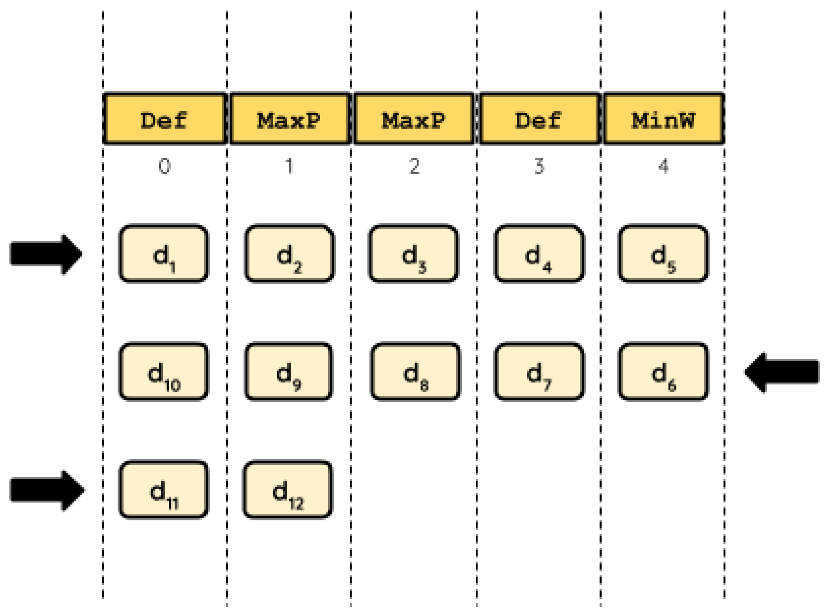


