A Multi-Strategy Improved Sparrow Search Algorithm for Solving the Node Localization Problem in Heterogeneous Wireless Sensor Networks

Abstract

Aiming at the problems of slow convergence and low accuracy of the traditional sparrow search algorithm (SSA), a multi-strategy improved sparrow search algorithm (ISSA) was proposed. Firstly, the golden sine algorithm was introduced in the location update of producers to improve the global optimization capability of SSA. Secondly, the idea of individual optimality in the particle swarm algorithm was introduced into the position update of investigators to improve the convergence speed. At the same time, a Gaussian disturbance was introduced to the global optimal position to prevent the algorithm from falling into the local optimum. Then, the performance of the ISSA was evaluated on 23 benchmark functions, and the results indicate that the improved algorithm has better global optimization ability and faster convergence. Finally, ISSA was used for the node localization of HWSNs, and the experimental results show that the localization algorithm with ISSA has a smaller average localization error than that of the localization algorithm with other meta-heuristic algorithms.

1. Introduction

Wireless sensor networks (WSNs) consist of a large number of miniature sensor nodes with low energy consumption, low price, and reliable performance [1]. They are often used in environmental monitoring, geological disaster warning, military reconnaissance, and other fields [2]. In these fields, location information is crucial, as data without geographic coordinate information are worthless [3]. Usually, a WSNs consists of hundreds or even thousands of sensor nodes, and designers cannot guarantee that all sensor nodes are of the same model. Further, the signal transmission power of the sensors generated by different sensor manufacturers will be different, which leads to the heterogeneity of the communication radius of sensor nodes. There may be various reasons for the formation of heterogeneous wireless sensor networks (HWSNs), but for localization techniques, the most important concern is the heterogeneity of the node communication radius. The localization problem of heterogeneous wireless sensor networks is similar to that of homogeneous wireless sensor networks in that the coordinates of unknown nodes are calculated by a specific localization algorithm using anchor nodes containing geographic coordinates within the network. However, unlike homogeneous wireless sensor networks, the heterogeneity of the node communication radius leads to a further increase in the localization error. Moreover, there are relatively few studies on conducting node localization of HWSNs.

Currently, researchers have proposed many localization algorithms. With the exception of the centroid localization algorithm, most localization algorithms can be divided into two stages: distance estimation and coordinate calculation. In the distance estimation phase, researchers can use the signal propagation time, the attenuation value of signal strength from the sending node to the receiving node, or the average hop distance and hop count between sensor nodes to calculate the distance between the unknown node and each anchor node [4]. In the coordinate calculation phase, the most commonly used method is the least-squares method (LS).

In recent years, meta-heuristic algorithms, which are known for their simplicity, flexibility, and spatial search capability, have provided a new idea for node coordinate calculation in WSNs. Liu et al. [5] replaced LS with a modified particle swarm algorithm (M-PSO) for the coordinate calculation of unknown nodes; when the error in the distance estimation stage was less than 10%, the error using M-PSO was 12.613 m less than that of the localization algorithm using LS. Chai et al. [6] proposed a parallel whale optimization algorithm to replace LS in the DV-Hop algorithm, and the obtained localization error was reduced by 8.4% compared with the DV-Hop algorithm. Cui et al. [7] improved the DV-Hop algorithm, made the discrete hop values continuous, and used the differential evolution algorithm (DE) to replace LS in the coordinate calculation stage. The positioning error of the algorithm was reduced by 70% compared with the DV-Hop algorithm. Although higher localization accuracy can be obtained using the meta-heuristic algorithm compared with LS, most of these studies focus on homogeneous wireless sensor networks, and few researchers have focused on HWSNs.

So far, not many results have been achieved on node localization of HWSNs. Assaf et al. [8] proposed a new expected hop progress (EHP) localization algorithm applicable to nodes with different transmission capabilities. The distance estimated by this algorithm in the distance estimation phase is closer to the real distance. However, the requirements for the potential forwarding area of the successor node are relatively high, and the communication radius of the sensor node cannot be too large. Wu et al. [9] optimized EHP and used elliptic distance to correct the distance calculated by the forward hop progress method and then used LS to find the coordinates of the unknown node. However, the node density required by the algorithm is too large. What is more, there is still room for improving the positioning accuracy of the nodes. Bhat et al. [10] proposed a minimum area localization algorithm for HWSNs combined with the Harris Hawk optimization algorithm, but the algorithm lacks a comparison with the use of other metaheuristic algorithms, and it is difficult to highlight the advantages of using HHO. No single meta-heuristic algorithm is suitable for the engineering applications used, so it is necessary to find a suitable metaheuristic algorithm in combination with specific application scenarios.

Meta-heuristic algorithms are mostly developed around physical phenomena, biological evolution, and group intelligence [11,12]. Among the many meta-heuristic algorithms, the most commonly used is the swarm intelligence optimization algorithm, such as the Harris Hawk optimization algorithm (HHO) [13], grey wolf optimizer (GWO) [14], butterfly optimization algorithm (BOA) [15], and so on. The sparrow search algorithm (SSA) [16] is a typical swarm intelligence optimization algorithm, which was proposed by Xue et al. in 2020. It has been widely used in many engineering fields, including UAV path planning [17], price prediction [18], and wind energy prediction [19]. In fact, the sparrow search algorithms suffer from the same problems as other meta-heuristic algorithms, such as low optimization-seeking accuracy and slow convergence. Thus, SSA needs to be improved. Yang et al. [20] used a chaotic mapping strategy to initialize the population and introduced adaptive weighting strategy and t-distribution variation strategy to balance the local exploration ability and global utilization ability of the algorithm. Yuan et al. [21] introduced centroid opposition learning, learning coefficients, and mutation operators in the original SSA to prevent SSA from falling into the local optima, and applied the improved algorithm to the control of distributed maximum power point tracking. Liu et al. [22] proposed a hybrid sparrow search algorithm based on constructing similarity, which overcomes the problem of the algorithm falling into a local optimum by introducing an improved chaotic mapping circle and t-distribution variation.

In summary, this paper compares the performance of 15 common meta-heuristic algorithms in node localization, and the comparison results are shown in Section 4. Then, SSA with better comprehensive performance is selected as the algorithm for the coordinate calculation stage, and SSA is improved with regard to its problems. Finally, the improved sparrow search algorithm (ISSA) is applied to the node localization of HWSNs. The main contributions of this paper are as follows:

• An improved sparrow search algorithm that incorporates the golden sine strategy, particle swarm optimal idea, and Gaussian perturbation is proposed. It shows a better performance in finding the optimal than the sparrow search algorithm and other comparative algorithms;
• ISSA is applied to the problem of solving the coordinates of unknown nodes in HWSNs. It achieves better localization accuracy compared with the localization algorithm using the remaining 15 meta-heuristic algorithms and LS.

The rest of this paper is organized as follows. In Section 2, the original SSA is introduced, and ISSA is presented to address the problems of slow convergence and low accuracy of SSA. In Section 3, simulation results are described and discussed. In Section 4, the application of ISSA in the node localization of HWSNs is introduced. Finally, Section 5 gives the summary of this paper and the direction of future work.

2. Basic SSA and Its Improvement

2.1. Basic SSA

SSA completes the spatial search by iteratively updating the position of each sparrow [16], and the entire population is divided into three categories: producer, scrounger, and investigator. The producers and scroungers each make up a certain proportion of the population and are dynamically updated according to the results of each iteration. However, the investigators are selected randomly from the whole population, usually at a rate of 10 to 20%. The details of the three categories are described as follows.

2.1.1. Updating Producer’s Location

The producers are primarily responsible for searching for food and guiding the movement of the entire population. When the warning value R₂ is less than the safety value ST, it indicates that no predators were discovered during the search, necessitating a broad search by the producers. When the warning value R₂ exceeds the safe value ST, the sparrow has encountered a predator and is obliged to guide all scroungers to a safe area. The location update equation of the producers is shown in Equation (1).

$$X_{i,j}^{t+1}=\{\begin{array}{l}{X}_{i,j}^t\cdot \exp \left(\frac{-i}{\alpha \cdot ite{r}_{\max }}\right)\mathrm{if}{R}_2<ST\\ X_{i,j}^t+Q\cdot L\hspace{1em}\hspace{1em}\hspace{1em} \mathrm{if}{R}_2\ge ST\end{array}$$

(1)

where t represents the current iteration, i and j are the individual numbers of the population and the dimensions of the solution problem, respectively, iter_max is the maximum number of iterations. $\alpha \in (0,1]$ represents a random, and Q denotes a random number following the normal distribution. L is a matrix of $1\times d$ in which each element is 1, where d represents the dimension of the solved problem. $X_{i,j}^t$ and $X_{i,j}^{t+1}$ are the position of the i-th sparrow’s j-th dimension in the t-th and (t + 1)-th iterations, respectively. $R_2\in (0,1]$ represents an alarm value, and $ST\in [0.5,1)$ represents the safety threshold.

2.1.2. Updating Scrounger’s Location

The remainder of the sparrow colony are scroungers whose primary function is to frequently monitor the producers. Once producers discover a source of good food, they will immediately abandon their current location in order to compete for it. Otherwise, the scroungers will go hungry and will be forced to fly to other locations in search of food. The location update equation of the scroungers is shown in Equation (2).

$$X_{i,j}^{t+1}=\{\begin{array}{l}Q\cdot \exp \left(\frac{X_{worst}^t-X_{i,j}^t}{i^2}\right)\mathrm{if}i>n/2\\ X_p^{t+1}+\left|X_{i,j}^t-X_p^{t+1}\right|\cdot A^{+}\cdot \mathrm{L}\mathrm{otherwise}\end{array}$$

(2)

where $X_{worst}^t$ represents the worst position in the t-th iteration and $X_p^{t+1}$ denotes the optimal position of the producer in the (t + 1)-th iteration. A is a matrix of 1 × d, in which the value of each element is randomly 1 or −1, and $A^{+}=A^{{\rm T}}{(A{A}^{{\rm T}})}^{-1}$. When $i>n/2$, it indicates that the sparrow is starving.

2.1.3. Updating Investigator’s Location

The investigators are primarily in charge of colony security. When they detect danger, sparrows on the colony’s periphery flee to a safe area. Those in the colony’s center, on the other hand, walk at random. The location update equation of the investigators is shown in Equation (3).

$$X_{i,j}^{t+1}=\{\begin{array}{l}{X}_{best}^t+\beta \cdot \left|X_{i,j}^t-X_{best}^t\right|\mathrm{if}{f}_i>f_g\\ X_{i,j}^t+K\left(\frac{\left|X_{i,j}^t-X_{worst}^t\right|}{(f_i-f_w)+\epsilon }\right)\mathrm{if}{f}_i=f_g\end{array}$$

(3)

where $X_{best}^t$ represents the global optimal position in the t-th iteration, $\beta$ denotes a normally distributed random number with mean 0 and variance 1, and k is a random number within [−1, 1]. $f_i$, $f_w$ and $f_g$ represent the fitness values of the i-th sparrow, the worst individual, and the best individual, respectively. $f_i>f_g$ means the sparrow is at the edge of the colony, and $f_i=f_g$ means the sparrow is in the middle of the colony.

According to Equation (1), the further back a producer is ranked in the fitness ranking, the more likely it is to fall into a local optimum. As a result, it is necessary to improve Equation (2) in order to improve the convergence accuracy of SSA. As shown in Equation (3), the vigilantes’ location updates are random, which is detrimental to SSA’s convergence speed.

2.2. Improved Sparrow Algorithm

2.2.1. Introduction of Golden Sine Strategy

The horizontal coordinates in Figure 1 represent producers sorted by fitness values, while the vertical coordinates represent the coefficient of variation of each producer’s position. As illustrated in Figure 1, the larger the producer’s ordinal number, the smaller the coefficient of variation of the position, which increases the probability of the producer falling into the local optimum. In summary, Equation (1) does not carry out a global search.

To improve the problem of the weak global search ability of the producers, the golden sine algorithm (Gold-SA) was introduced [23]. This algorithm traverses the whole search space by the relationship between the unit circle and the sine function on the one hand, and on the other hand, it gradually moves from the boundary of each dimension to the middle by the number of golden divisions until the best position for each dimension is found. Thus, in the paper, the golden sine algorithm is used to improve the global search ability of the producers in SSA. The equation of the discoverer position update after the introduction of the golden sine algorithm strategy is shown in Equation (4).

$$X=\{\begin{array}{l}{X}_{b,j}^t\cdot \left|\sin (r_1)\right|+r_2\cdot \sin (r_1)\cdot \left|x_1\cdot X-x_2\cdot X\right|\mathrm{if}{R}_2<ST\\ X_{i,j}^t+Q\cdot L\hspace{1em}\hspace{1em}\hspace{1em}\hspace{1em}\hspace{1em}\hspace{1em}\hspace{1em}\hspace{1em}\hspace{1em}\hspace{1em}\hspace{1em}\hspace{1em} \mathrm{if}{R}_2\ge ST\end{array}$$

(4)

where r₁ and r₂ are the random numbers within [0, 2π] and [0, π], respectively. $X_{b,j}^t$ represents the position of the j-th dimension of the optimal individual in the t-th iteration. The initial value of x₁ is $a\cdot (1-\tau )+b\cdot \tau$, and the initial value of x₂ is $a\cdot \tau +b\cdot (1-\tau )$, where τ is the golden mean and the initial value of a and b is −π and π, respectively. x₁, x₂, a, and b dynamically are updated as shown in Algorithm 1.

Algorithm 1: Pseudo-code for partial parameter update of Gold-SA
/* F represents the current fitness value, G represents the global optimal value, random1 and random2 represent random numbers between [0, 1] */
Input: x1←a·(1 − τ) + b·τ; x2←a·τ + b·(1 − τ); a←−π; b←π;
Output: x1, x2
1:	if (F < G) then
2:	b ← x2; x2 ← x1; x1 ← a·τ + b·(1 − τ);
3:	else
4:	a ← x1; x1 ← x2; x2 ← a·(1 − τ) + b·τ;
5:	end if
6:	if (x1 = x2) then
7:	a ← random1; b ← random2;
8:	x1 ← a·τ + b·(1 − τ); x2 ← a·(1 − τ) + b·τ;
9:	end if

2.2.2. Introduction of Individual Optimal Strategies

By comparing the fitness values of individuals to the global optimal, the sparrow population investigators contribute to the coordination of global exploration and local search in the whole space search. Further, the idea of individual optimality in the particle swarm algorithm can strengthen the convergence ability of the algorithm [24], and the investigators’ position update formula after introducing the optimal individual is as in Equation (5).

$$X_{i,j}^{t+1}=\{\begin{array}{l}{X}_{best}^t+\beta \cdot \left|X_{pi,j}^t-X_{best}^t\right|\mathrm{if}{f}_i>f_g\\ X_{pi,j}^t+K\left(\frac{\left|X_{pi,j}^t-X_{worst}^t\right|}{(f_{pi}-f_w)+\epsilon }\right)\mathrm{if}{f}_i=f_g\end{array}$$

(5)

where $X_{pi,j}^t$ represents the j-th dimensional value of the i-th sparrow’s historical optimal individual.

2.2.3. Gaussian Perturbation

The sparrow algorithm, like the majority of swarm intelligence optimization algorithms, suffer from the problem of falling into a local optimum, which results in poor searching accuracy. To address this issue, it is possible to use the fitness value of the population optimal individual to determine whether the algorithm is trapped in a local optimum [25]. If the global optimal individual’s fitness value is less than a threshold in two consecutive iterations, the algorithm is said to be trapped in a local optimum. At this time, a Gaussian random wandering strategy can be introduced to apply perturbation to the optimal position to help the algorithm to jump out of the local optimum. The improved way of updating the position of the investigators is shown in Equations (6)–(8).

$${\widehat{X}}_t=Gaussian(G_t,\sigma )$$

(6)

$$\sigma =\cos \left(\pi /2\cdot {\left(t/T\right)}^2\right)\cdot (G_t-X_t^{*})$$

(7)

$$G_t=\{\begin{array}{l}{\widehat{X}}_t,f({\overline{X}}_t)<f(G_t)\\ G_t,otherwise\end{array}$$

(8)

where $X_t$ is the position of the optimal individual after applying Gaussian perturbation at the t-th iteration, and $X_t^{*}$ is a random individual of the population.

3. Experimental Results and Analysis

HHO [13], SSA [16], PSO [24], Gold-SA [25], and artificial gorilla troops optimizer (GTO) [26] are selected as the comparison algorithms to verify the search performance of ISSA. The population size of all algorithms is set to 30, and the number of iterations is set to 500. In the ISSA proposed in this paper, the ratio of generators is 0.6, the ratio of discoverers is 0.7, and the ratio of vigilantes is 0.2. Meanwhile, Gaussian perturbation is introduced when the global optimum value is below the threshold 1.00 × 10⁻¹⁰ in two consecutive iterations. The parameters of the other algorithms are consistent with their literature. The whole experiment is divided into four parts: convergence accuracy analysis, convergence speed analysis, rank sum test, and complexity analysis. The simulation experiment described in this article was conducted on a Windows 11 64-bit operating system with an AMD Ryzen 7 5800H processor with Radeon Graphics 3.20 GHz, 16 GB of RAM, and MATLAB 2014B. All experimental results are the average values after 30 runs.

In this section, 23 test functions are selected from CEC’s benchmark functions, which are commonly used for optimization testing of meta-heuristic algorithms [16,27,28,29]. The functions F₁–F₇ are unimodal functions, the functions F₈–F₁₃ are multimodal functions, and the functions F₁₄–F₂₃ are fixed-dimension functions.

Table 1. Benchmark function.

Name	Formula of Functions	Dim	Range	Best
Sphere	$F_1(x)={\displaystyle \sum {}_{i=1}^n{x}_i^2}$	30	[100, 100]	0
Schwefel 2.22	$F_2(x)={\displaystyle \sum {}_{i=1}^n\left|x_i\right|}+{\prod }_{i=1}^n\left|x_i\right|$	30	[10, 10]	0
Schwefel 1.2	$F_3(x)={{\displaystyle \sum {}_{i=1}^n({\displaystyle \sum {}_{j-1}^i{x}_j})}}^2$	30	[100, 100]	0
Schwefel 2.21	$F_4(x)={\max }_i\{\left|x_i\right|,1\le i\le n\}$	30	[100, 100]	0
Rosenbrock	$F_5(x)={\displaystyle {\sum }_{i=1}^{n-1}[100{(x_{i+1}-x_i^2)}^2+{(x_i-1)}^2]}$	30	[30, 30]	0
Step	$F_6(x)={\displaystyle \sum {}_{i=1}^n{([x_i+0.5])}^2}$	30	[100, 100]	0
Quartic	$F_7(x)=i{x}_i^4+random[0,1]$	30	[128, 128]	0
Schwefel 2.26	$F_8(x)={\displaystyle \sum {}_{i=1}^n-x_i\sin }(\sqrt{\left|x_i\right|})$	30	[500, 500]	−418.9829 × n
Rastrigrin	$F_9(x)={\displaystyle \sum {}_{i=1}^n[x_i^2-10\cos (2\pi x_i)+10]}$	30	[5.12, 5.12]	0
Ackley	$F_{10}(x)=-20\exp \left(-0.2\sqrt{\frac{1}{n}{\displaystyle \sum {}_{i=1}^n{x}_i^2}}\right)-\exp \left(\frac{1}{n}{\displaystyle \sum {}_{i=1}^n\cos (2\pi x_i)}\right)+20+e$	30	[32, 32]	0
Griewank	$F_{11}(x)=\frac{1}{4000}{\displaystyle {\sum }_{i=1}^n{x}_i^2}-{\displaystyle {\prod }_{i=1}^n\cos (\frac{x_i}{\sqrt{i}})}+1$	30	[600, 600]	0
Penalized 1	$F_{12}(x)=\frac{\pi }{n}\{10{\sin }^2(\pi y_1)+{{\displaystyle {\sum }_{i=1}^{n-1}{(y_i-1)}^2[1+10{\sin }^2(\pi y_{i+1})]+(y_{n-1})}}^2\}+{\displaystyle {\sum }_{i=1}^{n}u(x_i,10,100,4)}$ $y_i=1+\frac{x_i+1}{4}\begin{array}{cc}& u=(x_i,a,k,m)=\{\begin{array}{c}k{(x_i-a)}^m,\begin{array}{cc}& x_i>a\end{array}\\ 0,\begin{array}{ccc}& & -a<x_i<a\end{array}\\ k{(-x_i-a)}^m,\begin{array}{cc}& x_i<a\end{array}\end{array}\end{array}$	30	[50, 50]	0
Penalized 2	$\begin{array}{l}{F}_{13}(x)=0.1\{{\sin }^2(3\pi x_i)+{\displaystyle {\sum }_{i=1}^n{(x_i-1)}^2[1+{\sin }^2(3\pi x_{i+1})]}+{(x_i-1)}^2(1+{\sin }^2(2\pi x_{i+1}))\}\\ +{\displaystyle {\sum }_{i=1}^{n}u(x_i,5,100,4)}\end{array}$	30	[50, 50]	0
Foxholes	$F_{14}(x)={(\frac{1}{500}+{\displaystyle {\sum }_{j=1}^{25}\frac{1}{j+{\displaystyle {\sum }_{i=1}^2{(x_i-a_{ij})}^6}}})}^{-1}$	2	[−65, 65]	1
Kowalik	$F_{15}(x)={{\displaystyle {\sum }_{i=1}^{11}\left[a_i-x_1(b_i^2+b_i{x}_2)/(b_i^2+b_i{x}_3+x_4)\right]}}^2$	4	[−5, −5]	0.00030
Six-Hump Gamel	$F_{16}(x)=4x_1^2-2.1x_1^4+\frac{1}{3}{x}_1^6+x_1{x}_2-4x_2^2+4x_2^4$	2	[−5, −5]	−1.0316
Branin	$F_{17}(x)={(x_2-\frac{5.1}{4{\pi }^2}{x}_1^2+\frac{5}{\pi }{x}_1-6)}^2+10(1-\frac{1}{8\pi })\cos x_1$	2	[−5, −5]	0.398
Goldstein-price	$\begin{array}{l}{F}_{18}(x)=[1+{(x_1+x_2+1)}^2(19-14x_1+3x_1^2-14x_2+6x_1{x}_2+3x_2^2)]\\ \hspace{1em}\hspace{1em}\hspace{1em} \ast [30+{(2x_1-3x_2)}^2\ast (18-32x_1+12x_1^2+48x_2-36x_1{x}_2+27x_2^2)]\end{array}$	2	[−2, 2]	3
Hartmann 3-D	$F_{19}(x)=-{\displaystyle {\sum }_{i=1}^4{c}_i\exp (-{{\displaystyle {\sum }_{j=1}^3{a}_{ij}(x_i-p_{ij})}}^2)}$	3	[1, 3]	−3.86
Hartmann 6-D	$F_{20}(x)=-{\displaystyle {\sum }_{i=1}^4{c}_i\exp (-{{\displaystyle {\sum }_{j=1}^6{a}_{ij}(x_i-p_{ij})}}^2)}$	6	[0, 1]	−3.32
Shekel 1	$F_{21}(x)=-{\displaystyle {\sum }_{i=1}^5{[(X-a_i){(X-a_i)}^T+c_i]}^{-1}}$	4	[0, 10]	−10.1532
Shekel 2	$F_{22}(x)=-{\displaystyle {\sum }_{i=1}^7{[(X-a_i){(X-a_i)}^T+c_i]}^{-1}}$	4	[0, 10]	−10.4029
Shekel 3	$F_{23}(x)=-{\displaystyle {\sum }_{i=1}^{10}{[(X-a_i){(X-a_i)}^T+c_i]}^{-1}}$	4	[0, 10]	−10.5364

lists the parameters of each function, including its expression, dimension, range, and optimal value.

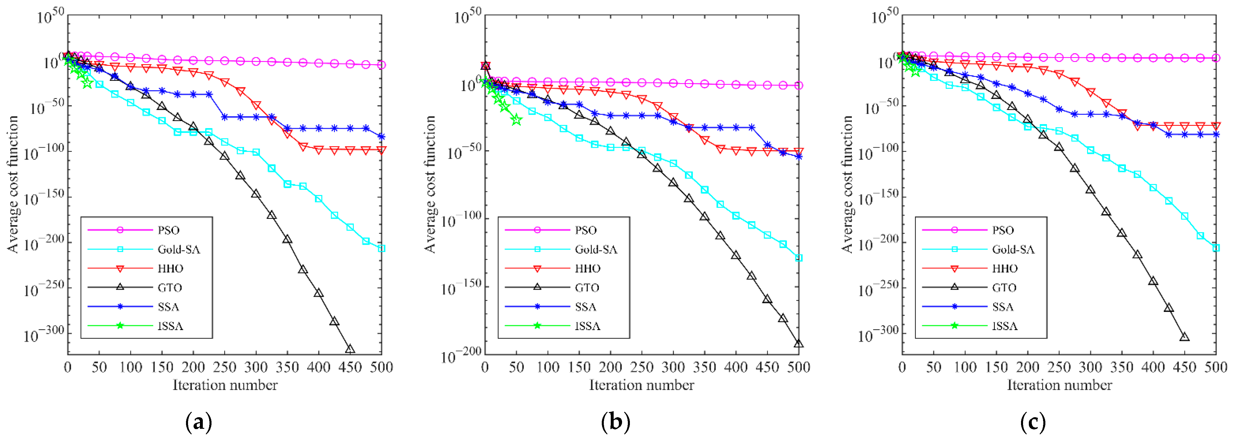
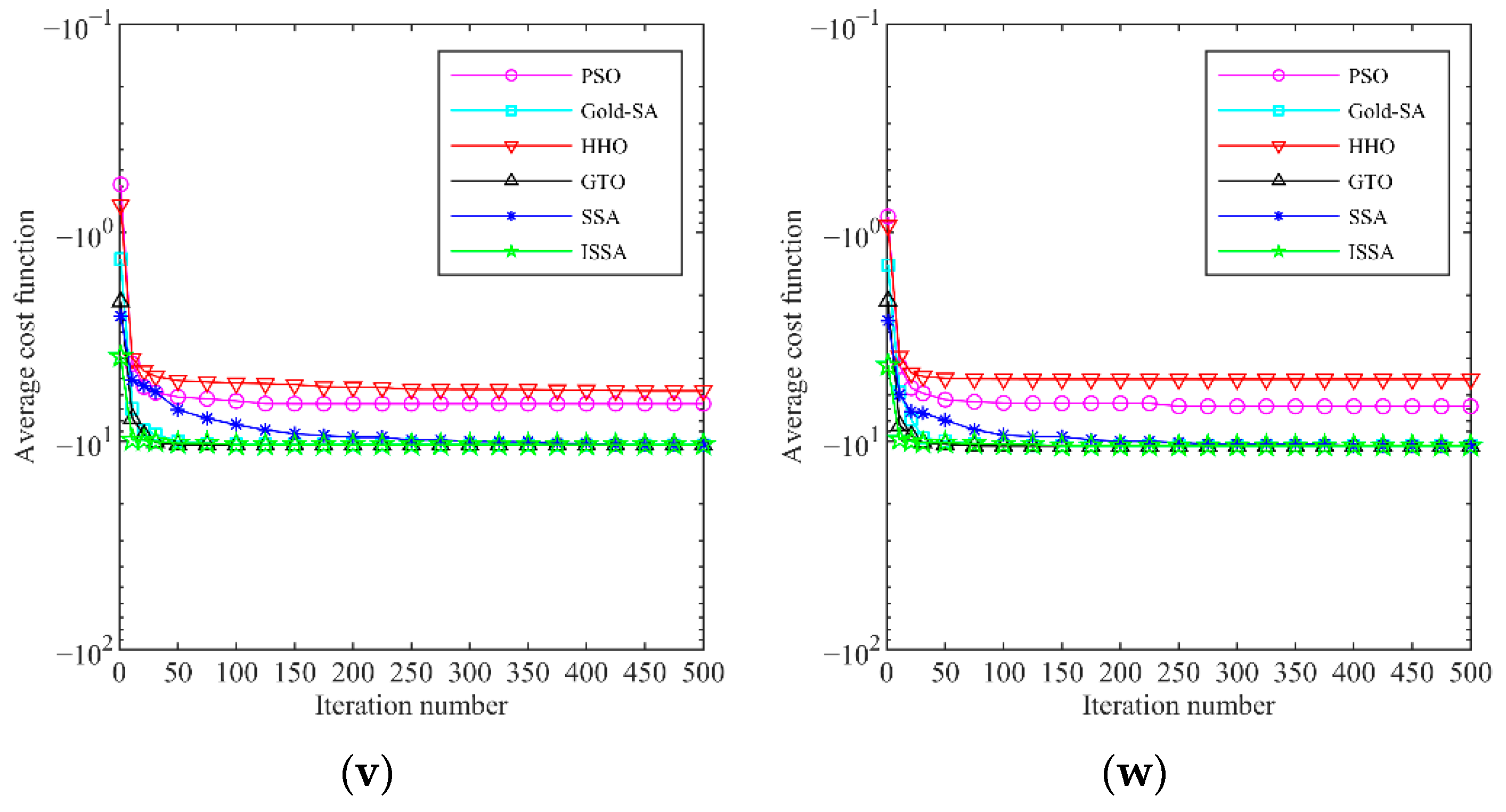
3.1. Convergence Accuracy Analysis

Table 2. Comparison of benchmark function results.

Function		PSO	Gold-SA	HHO	GTO	SSA	ISSA
F1	AVG	8.35 × 10−6	4.46 × 10−207	1.10 × 10 −98	0.0	1.11 × 10−84	0.0
	STD	8.80 × 10−6	0.0	4.65 × 10 −98	0.0	5.85 × 10−84	0.0
	p	4.13 × 10 −11(+)	9.64 × 10−2(−)	1.07 × 10−9(+)	7.27 × 10−8(+)	7.27 × 10−8(+)
F2	AVG	1.12 × 10−2	1.69 × 10−129	8.34 × 10−51	4.06 × 10−193	5.25 × 10−55	0.0
	STD	1.79 × 10−2	9.10 × 10−129	3.54 × 10−50	0.0	2.78 × 10−54	0.0
	p	4.46 × 10−11(+)	5.14 × 10−2(−)	2.45 × 10−10(+)	3.19 × 10−3(+)	2.24 × 10−11(+)
F3	AVG	4.13 × 10+02	1.47 × 10−206	4.36 × 10−72	0.0	5.32 × 10−82	0.0
	STD	1.28 × 10+03	0.0	2.34 × 10−71	0.0	2.82 × 10−81	0.0
	p	4.01 × 10−11(+)	7.42 × 10−2(−)	6.48 × 10−10(+)	2.01 × 10−07(+)	2.01 × 10−07(+)
F4	AVG	3.71 × 10−01	7.87 × 10−96	5.22 × 10−49	3.71 × 10−194	8.22 × 10−46	0.0
	STD	1.16 × 10−01	4.24 × 10−95	2.65 × 10−48	0.0	4.40 × 10−45	0.0
	p	3.00 × 10−11(+)	1.67 × 10−1(−)	1.69 × 10−8(+)	4.97 × 10−4(+)	1.93 × 10 −10(+)
F5	AVG	2.87 × 101	6.62 × 10−3	1.45 × 10−2	1.61	1.70 × 10−4	1.41 × 10−8
	STD	9.06	1.01 × 10−02	1.82 × 10−02	6.01	4.18 × 10−4	3.71 × 10−8
	p	3.02 × 10−11(+)	2.38 × 10−07(+)	8.15 × 10−11(+)	1.52 × 10−3(+)	6.07 × 10−11(+)
F6	AVG	5.02 × 10−6	2.31 × 10−4	1.37 × 10−4	1.77 × 10−7	3.90 × 10−7	2.46 × 10−11
	STD	5.90 × 10−6	3.07 × 10−4	2.19 × 10−4	1.80 × 10−7	5.04 × 10−7	7.98 × 10−11
	p	2.83 × 10−8(+)	5.49 × 10−11(+)	8.15 × 10 −11(+)	0.379(−)	4.50 × 10−11(+)
F7	AVG	7.57 × 10−2	2.16 × 10−4	1.73 × 10−4	9.01 × 10−5	3.67 × 10−4	6.57 × 10−5
	STD	2.68 × 10−2	2.84 × 10−4	2.24 × 10−4	8.64 × 10−5	3.27 × 10−4	4.81 × 10−5
	p	3.02 × 10−11(+)	1.44 × 10−3(+)	4.94 × 10−5(+)	9.06 × 10−8(+)	4.20 × 10−10(+)
F8	AVG	−2.70 × 103	−1.26 × 104	−1.26 × 104	−1.26 × 104	−9.34 × 103	−1.26 × 104
	STD	3.74 × 102	1.61 × 10−1	5.96 × 10−1	7.49 × 10−5	2.49 × 103	2.90 × 10−8
	p	3.02 × 10−11(+)	4.62 × 10−10(+)	1.55 × 10−9(+)	3.02 × 10−11(+)	2.91 × 10−11(+)
F9	AVG	52.1	0.0	0.0	0.0	0.0	0.0
	STD	12.2	0.0	0.0	0.0	0.0	0.0
	p	1.21 × 10−12(+)	NaN(=)	NaN(=)	NaN(=)	NaN(=)
F10	AVG	1.74 × 10−3	8.88 × 10−16	8.88 × 10−16	8.88 × 10−16	8.88 × 10−16	8.88 × 10−16
	STD	1.18 × 10−3	9.86 × 10−32	9.86 × 10−32	9.86 × 10−32	9.86 × 10−32	9.86 × 10−32
	p	1.21 × 10−12(+)	NaN(=)	NaN(=)	NaN(=)	NaN(=)
F11	AVG	42.0	0.0	0.0	0.0	0.0	0.0
	STD	5.85	0.0	0.0	0.0	0.0	0.0
	p	1.21 × 10−12(+)	NaN(=)	NaN(=)	NaN(=)	NaN(=)
F12	AVG	8.00 × 10−1	1.53 × 10−5	1.15 × 10−5	2.68 × 10−8	3.80 × 10−8	7.50 × 10−11
	STD	9.05 × 10−1	2.77 × 10−5	1.78 × 10−5	4.94 × 10−8	5.16 × 10−8	2.47 × 10−10
	p	3.02 × 10−11(+)	2.67 × 10−9(+)	8.10 × 10−10(+)	0.3871(−)	3.16 × 10−10(+)
F13	AVG	1.10 × 10−3	5.83 × 10−5	1.54 × 10−4	2.93 × 10−3	6.16 × 10−7	4.19 × 10−11
	STD	3.30 × 10−3	1.23 × 10−4	2.16 × 10−4	8.48 × 10−3	7.00 × 10−7	1.14 × 10−10
	p	3.87 × 10−1(−)	3.32 × 10−6(+)	4.20 × 10−10(+)	0.3555(−)	6.07 × 10−11(+)
F14	AVG	1.30	1.03	1.29	9.98 × 10−1	8.73	4.76
	STD	5.82 × 10−1	1.79 × 10−1	9.24 × 10−1	3.33 × 10−16	4.98	5.34
	p	7.44 × 10−10(+)	9.69 × 10−7(+)	2.05 × 10−6(+)	6.12 × 10−13(+)	4.20 × 10−5(+)
F15	AVG	4.75 × 10−4	4.00 × 10−4	3.50 × 10−4	3.99 × 10−4	3.21 × 10−4	3.08 × 10−4
	STD	2.76 × 10−4	2.42 × 10−4	3.20 × 10−5	2.75 × 10−4	2.55 × 10−5	7.64 × 10−7
	p	8.31 × 10−3(+)	1.09 × 10−5(+)	1.64 × 10−5(+)	7.64 × 10−8(+)	3.82 × 10−10(+)
F16	AVG	−1.03	−1.03	−1.03	−1.03	−1.03	−1.03
	STD	0.0	4.05 × 10−3	1.23 × 10−8	0.0	1.16 × 10−8	0.0
	p	1.21 × 10−12(+)	3.02 × 10−11(+)	8.88 × 10−1(−)	1.21 × 10−12(+)	1.21 × 10−12(+)
F17	AVG	3.98 × 10−1	4.00 × 10−1	3.98 × 10−1	3.98 × 10−1	3.98 × 10−1	3.98 × 10−1
	STD	1.11 × 10−16	1.28 × 10−2	4.06 × 10−5	1.11 × 10−16	1.32 × 10−8	3.72 × 10−16
	p	1.21 × 10−12(+)	3.02 × 10−11(+)	2.77 × 10−5(+)	1.21 × 10−12(+)	1.72 × 10−12(+)
F18	AVG	3.0	14.2	3.0	3.0	3.0	3.0
	STD	3.96 × 10−15	13.5	5.54 × 10−7	1.78 × 10−15	1.34 × 10−8	3.35 × 10−15
	p	6.32 × 10−12(+)	3.02 × 10−11(+)	6.63 × 10−1(−)	1.72 × 10−12(+)	4.08 × 10−12(+)
F19	AVG	−3.86	−3.8	−3.86	−3.86	−3.0	−3.86
	STD	2.66 × 10−15	8.01 × 10−2	3.04 × 10−3	2.66 × 10−15	5.07 × 10−5	2.66 × 10−15
	p	1.21 × 10−12(+)	3.34 × 10−11(+)	3.20 × 10−9(+)	1.21 × 10−12(+)	1.21 × 10−12(+)
F20	AVG	−3.25	−2.95	−3.1	−3.26	−3.26	−3.27
	STD	5.89 × 10−2	3.71 × 10−1	9.34 × 10−2	5.94 × 10−2	8.00 × 10−2	5.89× 10−2
	p	1.58 × 10−2(+)	9.83 × 10−8(+)	3.52 × 10−7(+)	3.485 × 10−3(+)	8.12 × 10−4(+)
F21	AVG	−6.31	−10.2	−5.19	−10.2	−10.2	−10.2
	STD	3.46	5.63 × 10−3	7.46 × 10−1	1.78 × 10−15	1.12 × 10−5	1.78 × 10−15
	p	5.00 × 10−1(−)	1.86 × 10−9(+)	3.02 × 10−11(+)	1.21 × 10−12(+)	1.21 × 10−12(+)
F22	AVG	−6.61	−10.4	−5.73	−10.4	−10.4	−10.4
	STD	3.8	5.11 × 10−3	1.67	0.0	3.02 × 10−4	0.0
	p	1(−)	1.96 × 10−10(+)	3.02 × 10−11(+)	1.21 × 10−12(+)	1.21 × 10−12(+)
F23	AVG	−6.81	−10.5	−5.05	−10.5	−10.5	−10.5
	STD	3.78	3.19 × 10−3	4.18 × 10−1	1.93 × 10−14	5.71 × 10−6	8.88 × 10−15
	p	1(−)	3.02 × 10−11(+)	3.02 × 10−11(+)	1.72 × 10−12(+)	1.21 × 10−12(+)

presents the average (AVG) and standard deviation (STD) of the average localization errors for the six meta-heuristics. Among them, R in Table 2 is explained in detail in Section 3.2.

According to Table 2, ISSA can find the optimal value in the unimodal functions F₁~F₄. This indicates that the introduction of the golden sine strategy significantly enhances the global optimality finding ability of the original SSSA. For the unimodal functions F₅~F₇, although the optimal values are not sought, their convergence accuracy is higher than that of the remaining four compared algorithms. For the multimodal functions F₈, although the mean value of ISSA is the same as Gold-SA, HHO, and GTO, the standard deviation of ISSA is much lower than that of Gold-SA, HHO, and GTO. Among the multimodal functions F₉~F₁₁, the convergence accuracy of ISSA is the same as that of Gold-SA, HHO, GTO, and SSA, and they can all converge to the optimal value. However, the convergence accuracy of ISSA is the best in all cases in the multimodal functions F₁₂ and F₁₃. For the fixed-dimension functions F₁₄~F₂₃, a total of seven best or tied best convergence accuracies were obtained for ISSA.

The ranking results of the six meta-heuristic algorithms are shown in Figure 2. The ranking is determined primarily by the average value of each algorithm; if the average value is identical, the ranking is determined by the standard deviation.

The radar plot shown in Figure 2 has 23 polar axes, and each polar axis represents 1 test function. Starting from the center point of the radar plot, there are six circles that expand outward in sequence, and the numbers on the circles represent the ranking of the algorithms. A closed polygon can be obtained by connecting the ranking points of each algorithm on the 23 test functions. The smaller the area of the polygon, the better the convergence performance of the algorithm. According to Figure 2, it can be seen that the area enclosed by ISSA is the smallest, which indicates that the convergence accuracy of ISSA is better than that of PSO, Gold-SA, HHO, GTO, and SSA.

3.2. Convergence Speed Analysis

The convergence curves for the six meta-heuristic algorithms on the 23 benchmark functions are depicted in Figure 3.

As shown in Figure 3, the convergence speed of ISSA in the unimodal functions F₁~F₇ is faster than that of the remaining five compared algorithms. In particular, ISSA can converge to the optimal value within 60 times in F₁~F₄. This indicates that the introduction of the individual optimal idea of PSO in the position update of the investigator greatly accelerates the convergence speed of the algorithm. For the multimodal functions F₈~F₁₃, the convergence speed of ISSA is also better than the remaining five comparison algorithms. Among the fixed-dimensional functions F₁₄~F₂₃, except for F₁₄, the convergence rate of ISSA is not weaker than that of PSO, Gold-SA, HHO, GTO, and SSA. In summary, the improved ISSA has a faster convergence speed.

3.3. Wilcoxon Rank Sum Test

García et al. [30] proposed that it is not sufficient to evaluate the performance of meta-heuristic algorithms using only the average and standard deviation. Therefore, it is essential to perform statistical tests. The Wilcoxon rank sum test, a binary hypothesis, determines whether there is a significant difference between two samples. It is assumed that H₀: the overall difference between the two samples is not significant, and H₁: there is a significant difference between the two samples. If the significance level between two samples is less than 0.05, then the H₀ hypothesis can be rejected; otherwise, the H₁ hypothesis is rejected. The significance level between such algorithms is denoted by p.

In this section, the results of one run of each meta-heuristic algorithm are taken as 1 element in the corresponding sample, and there are 30 elements in each set of samples. Combining the sample data of ISSA and the sample data of either metaheuristic algorithm can help to find the p value between them. NaN implies that the two samples are identical and cannot be tested with the Wilcoxon rank sum test, which indicates that the performance of the two sets of algorithms is the same. The p values on each benchmark function are shown in Table 2. The + located in parentheses after p represents a significant difference between the two samples, and − represents no significant difference. p combined with the AVG corresponding to the two algorithms can effectively determine the superiority of the algorithms. If AVG of ISSA is smaller than AVG of the comparison algorithm and H₁ holds, it means that ISSA performs better than the comparison algorithm. If AVG of ISSA is larger than AVG of the comparison algorithm and H₁ holds, the performance of ISSA is weaker than that of the comparison algorithm. If AVG of ISSA is the same as AVG of the comparison algorithm and H₁ holds, then the two algorithms have the same performance. In the remaining cases, it can be regarded as uncertain in terms of statistical significance.

Table 3. Statistical results of the performance advantages and disadvantages between ISSA and each algorithm.

ISSA and PSO	ISSA and Gold-SA	ISSA and HHO	ISSA and GTO	ISSA and SSA
14/1/4/4	10/1/8/4	13/1/7/2	6/1/13/3	13/0/10/0

a/b/c/d a, b, c denote the number of benchmark functions whose ISSA performance is better than, weaker than, or equal to the comparison algorithm, respectively. d denotes the number of benchmark functions that cannot be judged in terms of statistical significance.

gives the statistical results of the performance advantages and disadvantages between ISSA and the remaining five algorithms on 23 benchmark functions, respectively. As shown in Table 3, the performance of ISSA is better than that of SSA on 13 benchmark test functions, while the performance of ISSA is the same as that of SSA on the remaining 10 benchmark functions. This indicates that the proposed algorithm in this paper has achieved some success in terms of the performance of the optimization search. Compared with the GTO proposed by Abdollahzadeh et al. in 2021 [31], ISSA outperforms each other on all six benchmark functions and has the same performance on 13 benchmark functions. This indicates that ISSA still has some advantages over the recently proposed meta-heuristic algorithm.

3.4. Time Complexity Analysis

Let the population size of SSA and ISSA be N, the number of iterations be T_max, and the problem dimension be D. From Section 2, two algorithms differ only in the way they update different species of sparrows, and they have the same algorithmic complexity in the steps of population initialization, boundary check, position update, and sort update, all of which be $o(T_{\max }\cdot N\cdot D)$. Assuming that the proportions of producers, scroungers, and investigators in the sparrow population are r₁, r₂, and r₃, respectively, then in SSA, the time complexity of the location update of producers is $o(T_{\max }\cdot r_1\cdot N\cdot D)$, the time complexity of the location update of scroungers is $o(T_{\max }\cdot r_2\cdot N\cdot D)$, and the location update of investigators is $o(T_{\max }\cdot N\cdot D)$. The total time complexity of SSA is $o(T_{\max }\cdot N\cdot D)$.

In ISSA, the time complexity of the position update of the producer after introducing the golden sine strategy is $o(T_{\max }\cdot r_1\cdot N^2)$, and the position update of the investigators after introducing the particle swarm optimal idea is still $o(T_{\max }\cdot r_3\cdot N)$. In addition, the time complexity added by introducing Gaussian perturbation to the optimal sparrow individuals is $o(T_{\max }\cdot D)$. The total time complexity of ISSA is $o(T_{\max }\cdot N\cdot D\cdot (1+r_1\cdot N))$.

In summary, the time complexity of ISSA is slightly higher than that of SSA for the same number of iterations. However, the convergence speed of ISSA is fast, and the time consumption of ISSA may be reduced if no more changes in the search results are taken as the end condition. ISSA is more suitable for engineering applications that require high search accuracy and have lower requirements for computation time.

4. Application of ISSA in Node Location in HWSNs

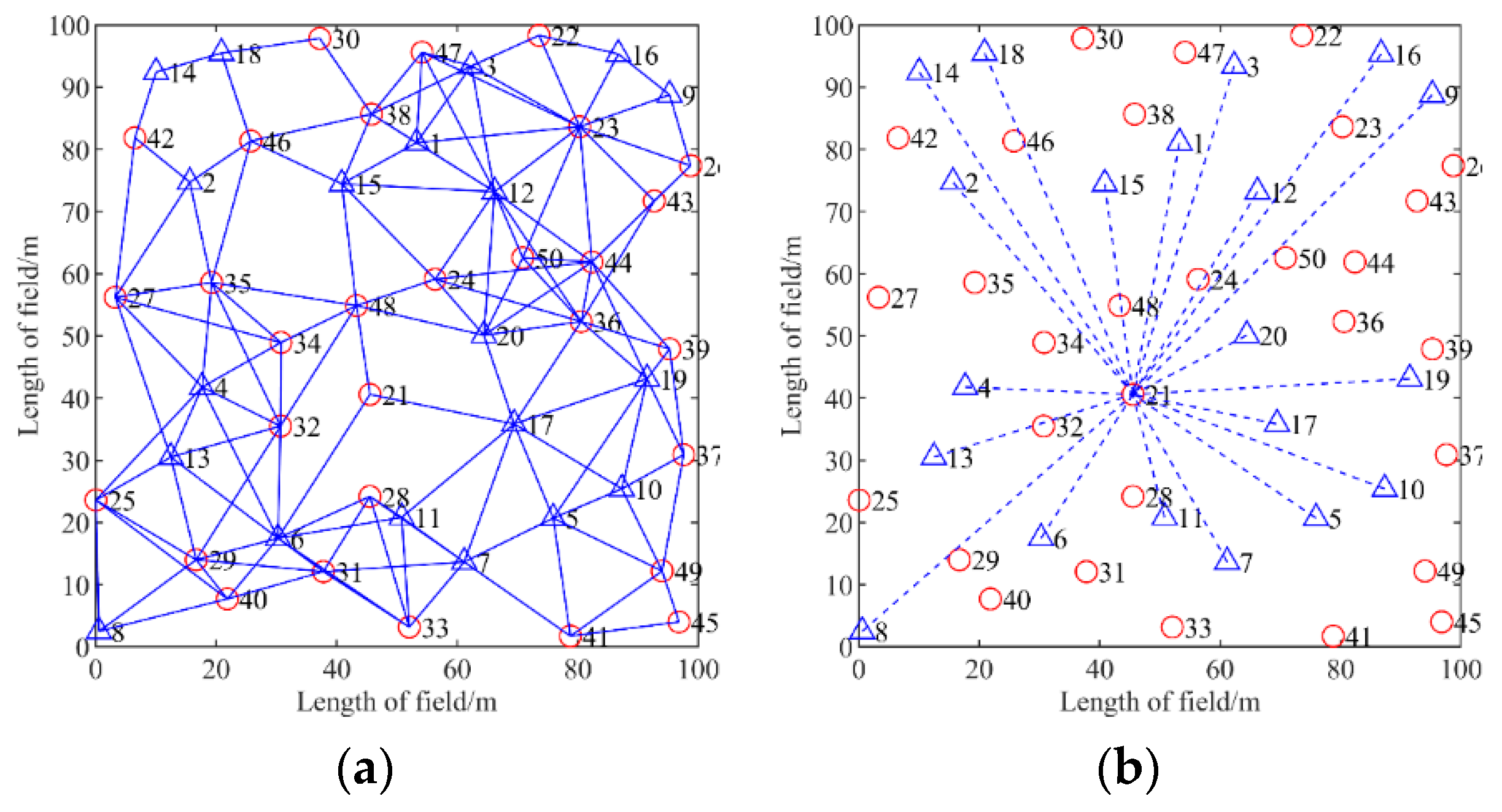
4.1. Node Localization Problem in HWSNs

The node localization of HWSNs can be divided into two stages: distance estimation and coordinate calculation. Once the distances from each anchor point to the unknown node are obtained in the distance estimation phase, the coordinate calculation of the unknown node can be transformed into an optimization problem, as shown in Equation (9). The dimension of this optimization problem is 2, and the theoretical optimal value is 0. Therefore, the problem can be solved by meta-heuristic algorithms.

$$F(x)={\displaystyle {\sum }_{j=1}^{Na}\left|\sqrt{{(x_1-a_j)}^2+{(x_2-b_j)}^2}-d_j\right|}$$

(9)

where Na indicates the number of anchor nodes, (a_j, b_j) represents the coordinates of the j-th unknown node, and d_j is the distance from the unknown node to the j-th anchor node.

4.2. Network Model

Figure 4a shows the network connection of 50 nodes in an area of 100 × 100 m², in which the number of anchor nodes represented by red ○ is 20, the number of unknown nodes represented by blue △ is 30, and the blue solid line represents the neighboring nodes can communicate with each other. In addition, the communication radius of each node is different. The node localization of HWSNs is to find out the coordinates of unknown nodes using the information of finite anchor nodes, such as the coordinates of each anchor point and the distance from each anchor point to the unknown node. The distance from each anchor node to the unknown node is shown in Figure 4b, in which blue dashed line indicates the distance from the anchor node to the unknown node.

4.3. Localization Steps

In this section, we replace the least-squares method of the localization algorithm with the meta-heuristic algorithm. The specific steps of the localization algorithm are as follows.

Step 1. Calculating the intersection area of the incoming neighbor

As shown in Figure 5a, when the intersection region of anchor nodes 1, 2, and 3 is used as the search space for meta-heuristic algorithms, the searching range can be narrowed, thus accelerating the convergence speed. However, because the intersection region of anchor points is an irregular graph, performing the calculation is difficult. To simplify computations, the communication region of each anchor point can be treated as a square, as illustrated in Figure 5b, and the intersection region of the incoming neighbor can then be calculated.

Step 2. Calculating the distance from the unknown node to each anchor node

In this step, the idea of the DV-Hop localization algorithm is adopted, and the product of hop count and hop distance between nodes is used as the distance from an unknown node to an anchor node. The hop distance formula is shown in Equation (10), and the distance from the unknown node to the anchor node is calculated in Equation (11).

$$Hopsiz{e}_i=\frac{{\displaystyle {\sum }_{i\ne k}\sqrt{{(x_i-x_k)}^2+{(y_i-y_k)}^2}}}{{\displaystyle {\sum }_{i\ne k}{h}_{ik}}}$$

(10)

$$d_{ij}=Hopsiz{e}_{ij}\cdot h_{ij}$$

(11)

where (x_i, y_i), (x_k, y_k) are the coordinates of anchors I and k, respectively, and h_ik represents the number of hops between anchors I and k. Hopsize_i is the hop distance of anchor I, Hopsize_ij denotes the hop distance of anchor I with the least number of hops from unknown node j, and d_ij is the distance between unknown node j to anchor i.

Step 3. Calculating coordinates of unknown node

To begin with, the fitness function is defined as in Equation (12). Then, the swarm intelligence optimization algorithm is used to find the unknown node coordinates, with the coordinates with the lowest fitness values being selected as the unknown node coordinates. If the distance value in Step 2 is guaranteed to be constant, the higher the performance of the chosen swarm intelligence optimization algorithm, the more accurate the positioning.

$$fitnes{s}_j={\displaystyle {\sum }_{i=1}^{Na}\left|\sqrt{{({\tilde{x}}_j-x_i)}^2+{({\tilde{y}}_j-y_i)}^2}-d_{ij}\right|}$$

(12)

where j represents the unknown node numbers, N_a is the total number of anchors, and (x_j, y_j) represents the coordinates of unknown nodes randomly generated.

4.4. Performance Evaluation

To verify the superiority of ISSA for node localization in HWSNs, we compared it with LS and 15 other meta-heuristic algorithms, including HHO [13], GWO [14], BOA [15], SSA [16], Gold-SA [23], PSO [24], GTO [26], sine cosine algorithm (SCA) [31], DE [32], Archimedes optimization algorithm (AOA) [33], whale optimization algorithm (WOA) [34], elephant herding optimization (EHO) [35], marine predators algorithm (MPA) [36], tunicate swarm algorithm (TSA) [37], and Coot optimization algorithm (COOT) [38]. All meta-heuristic algorithms have a population size of 30, an iteration number of 50, and other parameters that are consistent with their original literature. The area of HWSNs is 100 × 100 m², the number of anchor nodes is 25, and the node communication radius is a random value within [15,29], and the normalized root mean square error (NRMSE) is used to evaluate the positioning performance as shown in Equation (13).

$$NRMSE=\frac{1}{Nu}{\displaystyle {\sum }_{j=1}^{Nu}\frac{1}{r_j}}\sqrt{{(x_j-{\tilde{x}}_j)}^2+{(y_j-{\tilde{y}}_j)}^2}$$

(13)

where Nu represents the number of unknown nodes and $(x_i,y_i)$, and $({\tilde{x}}_j,{\tilde{y}}_j)$ are the true and estimated coordinates of the unknown node, respectively.

The NRMSE and the time required to compute the coordinates of unknown nodes using LS or different meta-heuristic algorithms when all nodes in HWSNs have the same coordinate positions are shown in

Table 4. Positioning results of 17 algorithms.

	NRMSE			Time
	AVG	STD	Rank	AVG	STD	Rank
LS	0.5557	0.0945	17	0.0903	0.0358	1
PSO	0.4545	0.0592	15	1.0545	0.2449	5
DE	0.4178	0.0610	4	1.4722	0.1060	13
SCA	0.4252	0.0602	6	1.1997	0.1844	9
Gold-SA	0.4245	0.0633	5	1.1809	0.2874	8
AOA	0.4408	0.0606	8	0.9484	0.3666	3
GWO	0.4414	0.0572	12	1.1724	0.1841	7
WOA	0.4448	0.0574	13	1.1524	0.1596	6
EHO	0.5457	0.0484	16	1.3273	0.1379	10
BOA	0.4389	0.0542	7	1.4387	0.0863	11
SSA	0.4168	0.0596	3	0.9542	0.1997	4
MPA	0.4409	0.0595	10	3.1366	0.4165	16
TSA	0.4414	0.0572	11	0.7694	0.0841	2
COOT	0.4409	0.0569	9	1.4474	0.4420	12
HHO	0.4453	0.0548	14	2.3375	0.3184	15
GTO	0.4151	0.0611	2	10.3031	0.4517	17
ISSA	0.4138	0.0590	1	1.6637	0.4558	14

. As far as the NRMSE is concerned, the average localization error of LS is higher than that of all other metaheuristic algorithms, reaching 55.57%. This indicates that using meta-heuristic algorithms to solve the coordinates of unknown nodes can indeed reduce the localization error of the nodes. The localization error obtained using different metaheuristic algorithms also varies. The best-performing ISSA has a 13.19% reduction in the average positioning error compared with the worst performing EHO. The top four average positioning errors are ISSA, GTO, SSA, and DE in order, and their average positioning errors are 41.38%, 41.51%, 41.68%, and 41.78%, respectively. Although the NEMSE of the top four meta-heuristic algorithms is not very different, there is a big difference in the positioning time required by each of them.

In terms of search time, LS takes the shortest time of 0.04 s, while GTO takes the longest time of 10.3 s. The times required for ISSA, GTO, SSA, and DE localization are 1.66 s, 10.3 s, 0.95 s, and 1.47 s, respectively. It can be seen that, when solving the node coordinates of HWSNs, it is difficult to achieve both accuracy and time optimality. However, the localization accuracy is the most critical index in the node localization of HWSNs. Within a certain range, the search time requirement can be reduced appropriately. In summary, the ISSA proposed in this paper is more suitable for node localization in HWSNs.

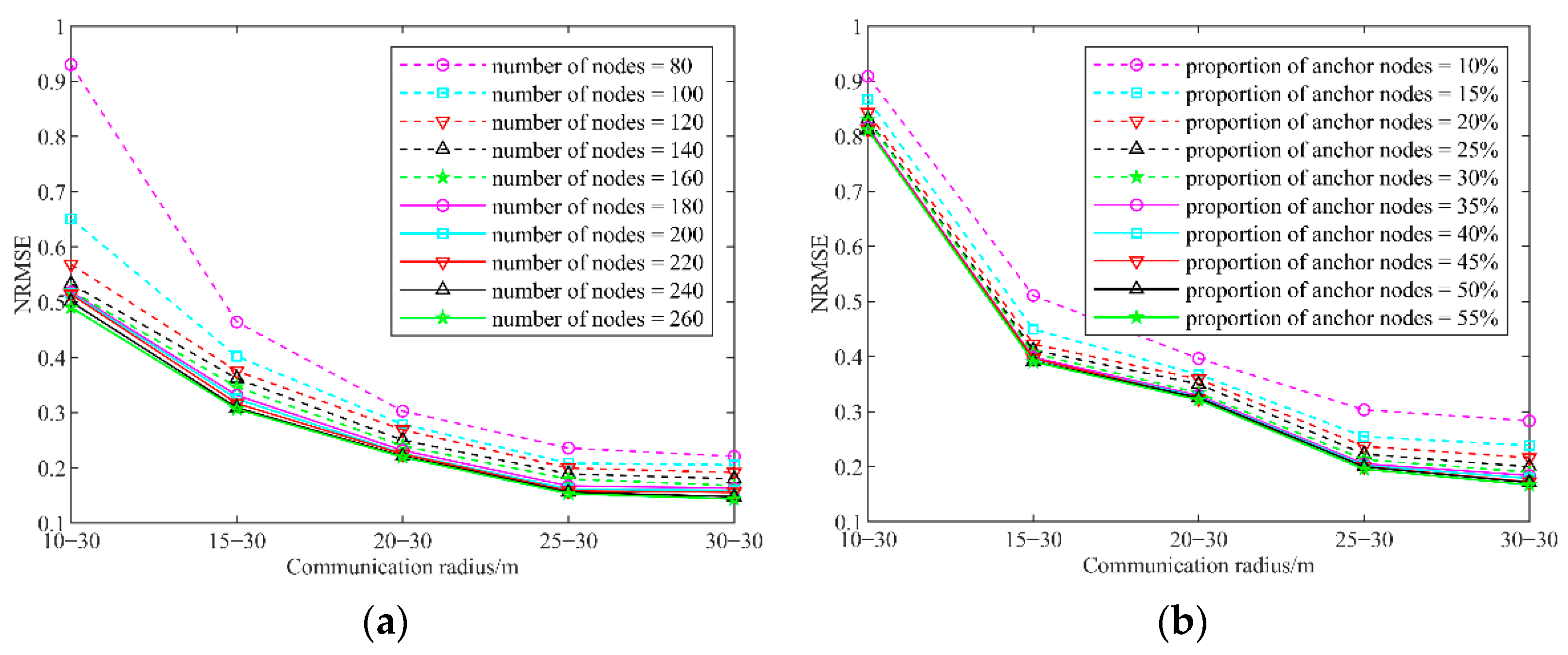
4.5. Effect of Parameter Variation on Localization Accuracy in HWSNs

Figure 6 depicts the effect on NRMSE when the number of nodes and the ratio of anchor points are varied in a deployment area of 100 × 100 m². The 10–30 in Figure 6a,b indicates that the communication radius of the nodes is a random value within [10, 30], and 30–30 indicates that the communication radius of the nodes is all 30 m. The ratio of anchor points in Figure 6a is 25, and the total number of nodes in Figure 6b is 100. ISSA is used to calculate the coordinates of unknown nodes with 50 iterations, and the number of individuals in the population is 30.

From Figure 6, the NRMSE decreases as the heterogeneous range of node communication radius decreases, regardless of the number of nodes and the ratio of anchor points taken. From Figure 6a, the NRMSE decreases continuously when the number of nodes increases sequentially, but the magnitude of its decrease also becomes smaller. When the number of nodes increases to 160, the average variation of NRMSE on different communication intervals is less than 1%. From Figure 6b, the NRMSE also decreases as the proportion of anchor points increases, but the magnitude of its decrease also becomes slower. When the anchor point ratio is 25%, the reduction of NRMSE tends toward 0. Therefore, the optimal number of nodes is 160, and the optimal anchor point ratio is 25% when using the localization algorithm described in this section to solve the localization problem.

5. Conclusions

In this paper, for the node localization problem in HWSNs, we compared the localization accuracy and localization time consumption of 15 common meta-heuristic algorithms and found that the comprehensive performance of SSA is the best. Thus, a multi-strategy improved sparrow search algorithm is proposed to address the problems of SSA. To improve the global exploration capability of SSA, the golden sine strategy was introduced into the producer’s position update method. Meanwhile, to accelerate the convergence speed of SSA, the idea of individual optimality of particle swarm was introduced to the location update method of the investigator. To prevent SSA from falling into local optimality, Gaussian perturbation was applied to the globally optimal sparrow individuals. A total of 23 benchmark functions and 5 meta-heuristics were chosen to evaluate ISSA’s optimization performance. In terms of the average value and standard deviation of the search results, ISSA achieved first place or was tied for first place on a total of 20 benchmark functions. Except for F14, the convergence speed of ISSA is not weaker than the rest of the comparison algorithms. In addition, the Wilcoxon rank sum test and the average value were combined in order to evaluate the performance of the algorithms. From a statistical point of view, the number of benchmark functions in which ISSA outperforms PSO, Gold-SA, HHO, GTO, and SSA is 14, 10, 13, 6, and 13, respectively.

Finally, ISSA was used to solve the problem of solving unknown node coordinates for HWSNs coordinate calculation. Simulation experiments showed that the localization accuracy obtained using ISSA to compute node coordinates is the best among the 15 meta-heuristic algorithms and LS, and it reduces the localization error by 14.19% compared with LS. Changing the internal parameters of HWSNs, it can be found that increasing the number of nodes and increasing the proportion of anchor nodes can improve the accuracy of the localization algorithm. However, when the number of nodes reaches 160 and the proportion of anchor nodes reaches 25%, the enhancement effect will be significantly weakened.

Unfortunately, applying the proposed ISSA to the node localization of HWSNs improves the localization accuracy but also increases the time required for localization. In our future work, we will further optimize the search mechanism of ISSA to reduce the search time during node localization. In addition, we will also focus on the distance estimation of the first stage of the HWSNs localization problem to further improve the localization accuracy.

References

1. Phoemphon, S.; So-In, C.; Leelathakul, N. Improved distance estimation with node selection localization and particle swarm optimization for obstacle-aware wireless sensor networks. Expert Syst. Appl. 2021, 175, 114773. [Google Scholar] [CrossRef]
2. Nemer, I.; Sheltami, T.; Shakshuki, E.; Elkhail, A.A.; Adam, M. Performance evaluation of range-free localization algorithms for wireless sensor networks. Pers. Ubiquit. Comput. 2021, 25, 177–203. [Google Scholar] [CrossRef]
3. Nithya, B.; Jeyachidra, J. Low-cost localization technique for heterogeneous wireless sensor networks. Int. J. Commun. Syst. 2021, 34, e4733. [Google Scholar] [CrossRef]
4. Tu, Q.; Liu, Y.; Han, F.; Liu, X.; Xie, Y. Range-free localization using Reliable Anchor Pair Selection and Quantum-behaved Salp Swarm Algorithm for anisotropic Wireless Sensor Networks. Ad Hoc Netw. 2021, 113, 102406. [Google Scholar] [CrossRef]
5. Liu, Z.K.; Liu., Z. Node self-localization algorithm for wireless sensor networks based on modified particle swarm optimization. In Proceedings of the 27th Chinese Control and Decision Conference (2015 CCDC), Qingdao, China, 23–25 May 2015; pp. 5968–5971. [Google Scholar]
6. Chai, Q.; Chu, S.; Pan, J.; Hu, P.; Zheng, W. A parallel WOA with two communication strategies applied in DV-Hop localization method. EURASIP J. Wirel. Commun. 2020, 2020, 50. [Google Scholar] [CrossRef]
7. Cui, L.; Xu, C.; Li, G.; Ming, Z.; Feng, Y.; Lu, N. A high accurate localization algorithm with DV-Hop and differential evolution for wireless sensor network. Appl. Soft Comput. 2018, 68, 39–52. [Google Scholar] [CrossRef]
8. Assaf, A.E.; Zaidi, S.; Affes, S.; Kandil, N. Low-Cost Localization for Multihop Heterogeneous Wireless Sensor Networks. IEEE Trans. Wirel. Commun. 2016, 15, 472–484. [Google Scholar] [CrossRef]
9. Wu, W.; Wen, X.; Xu, H.; Yuan, L.; Meng, Q. Efficient range-free localization using elliptical distance correction in heterogeneous wireless sensor networks. Int. J. Distrib. Sens. Netw. 2018, 14, 1–9. [Google Scholar] [CrossRef] [Green Version]
10. Bhat, S.J.; Venkata, S.K. An optimization based localization with area minimization for heterogeneous wireless sensor networks in anisotropic fields. Comput. Netw. 2020, 179, 107371. [Google Scholar] [CrossRef]
11. Goel, L. An extensive review of computational intelligence-based optimization algorithms: Trends and applications. Soft Comput. 2020, 24, 16519–16549. [Google Scholar] [CrossRef]
12. Zhang, J.; Wang, J.S. Improved Whale Optimization Algorithm Based on Nonlinear Adaptive Weight and Golden Sine Operator. IEEE Access 2020, 8, 77013–77048. [Google Scholar] [CrossRef]
13. Heidari, A.A.; Mirjalili, S.; Faris, H.; Aljarah, I.; Mafarja, M.; Chen, H. Harris hawks optimization: Algorithm and applications. Future Gener. Comput. Syst. 2019, 97, 849–872. [Google Scholar] [CrossRef]
14. Mirjalili, S.; Mirjalili, S.M.; Lewis, A. Grey Wolf Optimizer. Adv. Eng. Softw. 2014, 69, 46–61. [Google Scholar] [CrossRef] [Green Version]
15. Arora, S.; Singh, S. Butterfly optimization algorithm: A novel approach for global optimization. Soft Comput. 2018, 23, 715–734. [Google Scholar] [CrossRef]
16. Xue, J.; Shen, B. A novel swarm intelligence optimization approach: Sparrow search algorithm. Syst. Sci. Control. Eng. 2020, 8, 22–34. [Google Scholar] [CrossRef]
17. Liu, G.; Shu, C.; Liang, Z.; Peng, B.; Cheng, L. A Modified Sparrow Search Algorithm with Application in 3d Route Planning for UAV. Sensors 2021, 21, 1224. [Google Scholar] [CrossRef]
18. Zhou, J.; Chen, D. Carbon Price Forecasting Based on Improved CEEMDAN and Extreme Learning Machine Optimized by Sparrow Search Algorithm. Sustainability 2021, 13, 4896. [Google Scholar] [CrossRef]
19. An, G.; Jiang, Z.; Chen, L.; Cao, X.; Li, Z.; Zhao, Y.; Sun, H. Ultra Short-Term Wind Power Forecasting Based on Sparrow Search Algorithm Optimization Deep Extreme Learning Machine. Sustainability 2021, 13, 10453. [Google Scholar] [CrossRef]
20. Yang, X.; Liu, J.; Liu, Y.; Xu, P.; Yu, L.; Zhu, L.; Chen, H.; Deng, W. A Novel Adaptive Sparrow Search Algorithm Based on Chaotic Mapping and T-Distribution Mutation. Appl. Sci. 2021, 11, 11192. [Google Scholar] [CrossRef]
21. Yuan, J.; Zhao, Z.; Liu, Y.; He, B.; Wang, L.; Xie, B.; Gao, Y. DMPPT Control of Photovoltaic Microgrid Based on Improved Sparrow Search Algorithm. IEEE Access 2021, 9, 16623–16629. [Google Scholar] [CrossRef]
22. Liu, J.; Wang, Z. A Hybrid Sparrow Search Algorithm Based on Constructing Similarity. IEEE Access 2021, 9, 117581–117595. [Google Scholar]
23. Tanyildizi, E.; Demir, G. Golden Sine Algorithm: A Novel Math-Inspired Algorithm. Adv. Electr. Comput. Eng. 2017, 17, 71–78. [Google Scholar] [CrossRef]
24. Kennedy, J.; Eberhart, R. Particle swarm optimization. In Proceedings of the ICNN’95—International Conference on Neural Networks, Perth, WA, Australia, 27 November–1 December 1995; pp. 1942–1948. [Google Scholar]
25. Xiao, S.; Wang, H.; Wang, W.; Huang, Z.; Zhou, X.; Xu, M. Artificial bee colony algorithm based on adaptive neighborhood search and Gaussian perturbation. Appl. Soft Comput. 2021, 100, 106955. [Google Scholar] [CrossRef]
26. Abdollahzadeh, B.; Soleimanian Gharehchopogh, F.; Mirjalili, S. Artificial gorilla troops optimizer: A new nature-inspired metaheuristic algorithm for global optimization problems. Int. J. Intell. Syst. 2021, 36, 5887–5958. [Google Scholar] [CrossRef]
27. Zhang, M.; Wang, D.; Yang, J. Hybrid-Flash Butterfly Optimization Algorithm with Logistic Mapping for Solving the Engineering Constrained Optimization Problems. Entropy 2022, 24, 525. [Google Scholar] [CrossRef]
28. Jamil, M.; Yang, X. A literature survey of benchmark functions for global optimisation problems. Int. J. Math. Model. Numer. Optim. 2013, 4, 150–194. [Google Scholar] [CrossRef] [Green Version]
29. Rashedi, E.; Nezamabadi-Pour, H.; Saryazdi, S. GSA: A Gravitational Search Algorithm. Inf. Sci. 2009, 179, 2232–2248. [Google Scholar] [CrossRef]
30. García, S.; Molina, D.; Lozano, M.; Herrera, F. A study on the use of non-parametric tests for analyzing the evolutionary algorithms’ behaviour: A case study on the CEC’2005 Special Session on Real Parameter Optimization. J. Heuristics 2009, 15, 617–644. [Google Scholar] [CrossRef]
31. Mirjalili, S. SCA: A Sine Cosine Algorithm for solving optimization problems. Knowl.-Based Syst. 2016, 96, 120–133. [Google Scholar] [CrossRef]
32. Storn, R.; Price, K. Differential Evolution—A Simple and Efficient Heuristic for global Optimization over Continuous Spaces. J. Glob. Optim. 1997, 11, 341–359. [Google Scholar] [CrossRef]
33. Hashim, F.A.; Hussain, K.; Houssein, E.H.; Mabrouk, M.S.; Al-Atabany, W. Archimedes optimization algorithm: A new metaheuristic algorithm for solving optimization problems. Appl. Intell. 2020, 51, 1531–1551. [Google Scholar] [CrossRef]
34. Mirjalili, S.; Lewis, A. The Whale Optimization Algorithm. Adv. Eng. Softw. 2016, 95, 51–67. [Google Scholar] [CrossRef]
35. Wang, G.-G.; Deb, S.; Coelho, L.d.S. Elephant Herding Optimization. In Proceedings of the 2015 3rd International Symposium on Computational and Business Intelligence (ISCBI), Bali, Indonesia, 7–9 December 2015; pp. 1–5. [Google Scholar]
36. Faramarzi, A.; Heidarinejad, M.; Mirjalili, S.; Gandomi, A.H. Marine Predators Algorithm: A nature-inspired metaheuristic. Expert Syst. Appl. 2020, 152, 113377. [Google Scholar] [CrossRef]
37. Kaur, S.; Awasthi, L.K.; Sangal, A.L.; Dhiman, G. Tunicate Swarm Algorithm: A new bio-inspired based metaheuristic paradigm for global optimization. Eng. Appl. Artif. Intell. 2020, 90, 103541. [Google Scholar] [CrossRef]
38. Naruei, I.; Keynia, F. A new optimization method based on COOT bird natural life model. Expert Syst. Appl. 2021, 183, 115352. [Google Scholar] [CrossRef]
Figure 1. Relationship between location variation coefficient and numbering of producers.
Applsci 12 05080 g001
Figure 2. Radar chart of sort of algorithm.
Applsci 12 05080 g002
Figure 3. Convergence curve of benchmark function: (a) F1: Sphere; (b) F2: Schwefel 2.22; (c) F3: Schwefel 1.2; (d) F4: Schwefel 2.21; (e) F5: Rosenbrock; (f) F6: Step; (g) F7: Quartic; (h) F8: Schwefel 2.26; (i) F9: Rastrigrin; (j) F10: Ackley; (k) F11: Griewank; (l) F12: Penalized 1; (m) F13: Penalized 2; (n) F14: Foxholes; (o) F15: Kowalik; (p) F16: Six-Hump Gamel; (q) F17: Branin; (r) F18: Goldstein-price; (s) F19: Hartmann 3-D; (t) F20: Hartmann 6-D; (u) F21: Shekel 1; (v) F22: Shekel 2; (w) F23: Shekel 3.
Applsci 12 05080 g003aApplsci 12 05080 g003bApplsci 12 05080 g003cApplsci 12 05080 g003d
Figure 4. Heterogeneous wireless sensor network model: (a) network connections; (b) distance from all anchor nodes to unknown node 21.
Applsci 12 05080 g004
Figure 5. Impact of heterogeneity of communication radius on network communication: (a) original communication radius; (b) square communication radius.
Applsci 12 05080 g005
Figure 6. Effect of parameter variation on positioning accuracy: (a) change in number of nodes; (b) change of anchor node ratio.
Applsci 12 05080 g006