An Algorithm for Arranging Operators to Balance Assembly Lines and Reduce Operator Training Time

Abstract

Industry 4.0 is transforming how costs, including labor costs, are managed in manufacturing and remanufacturing systems. Managers must balance assembly lines and reduce the training time of workstation operators to achieve sustainable operations. This study’s originality lies in its use of an algorithm to balance an assembly line by matching operators to workstations so that the line’s workstations achieve the same targeted output rates. First, the maximum output rate of the assembly line is found, and then the number of operators needed at each workstation is determined. Training time is reduced by matching operators’ training and skills to workstations’ skill requirements. The study obtains a robust, cluster algorithm based on the concept of group technology, then forms operator skill cells and determines operator families. Four numerical examples are presented to demonstrate the algorithm’s implementation. The proposed algorithm can solve the problem of arranging operators to balance assembly lines. Managers can also solve the problem of worker absences by assigning more than one operator with the required skillset to each workstation and rearranging them as needed.

1. Introduction

Netessine and Taylor [1] demonstrated that expensive production technology usually leads to low product prices and may simultaneously lead to high-quality products. However, the product price is usually proportional to the product cost, part of which is labor cost. Assembly line balancing (ALB) is a crucial part of production/operations management [2]. On most mass-production assembly lines, workers repetitively perform a set of tasks predefined by using assembly line balancing techniques [3], which assign a number of work elements to various workstations to maximize the assembly line’s balancing efficiency [4]. A balancing of tasks across the workstations results in the optimization of a given objective function without violating preceding constraints [5]. An unbalanced assembly line can be dangerous. For example, an operator without adequate training or who is focused on personal problems can cause an accident, decrease the efficiency of the assembly line, and increase production costs. Assembly lines maximize assembly operations, and most manufacturing plants have one or more lines, making assembly line balancing one of the oldest challenges in industry [6]. Moreover, a balanced assembly line can reduce a factory’s work-in-process (WIP) inventory. Kim et al. [7] suggested a mathematically mixed integer programming model that accounts for the WIP balance and setup time in a semiconductor fabrication line. Maximum productivity and minimum load smoothness are benefits of solving the assembly line balancing problem (ALBP) [8,9].

Many types of production lines exist. Kuroda [10] presented a robust design for a cellular-line production system with unreliable facilities. A cellular-line production system comprises multiple flow shops, which are individual sets composed of functionally different facilities. Kuroda grouped facilities that perform similar operations.

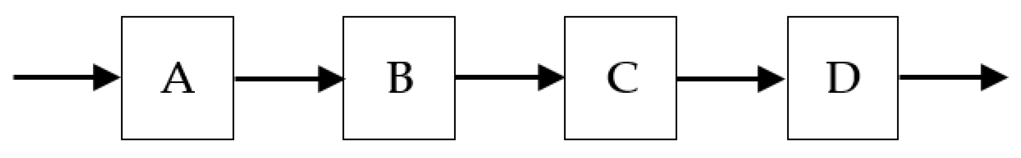
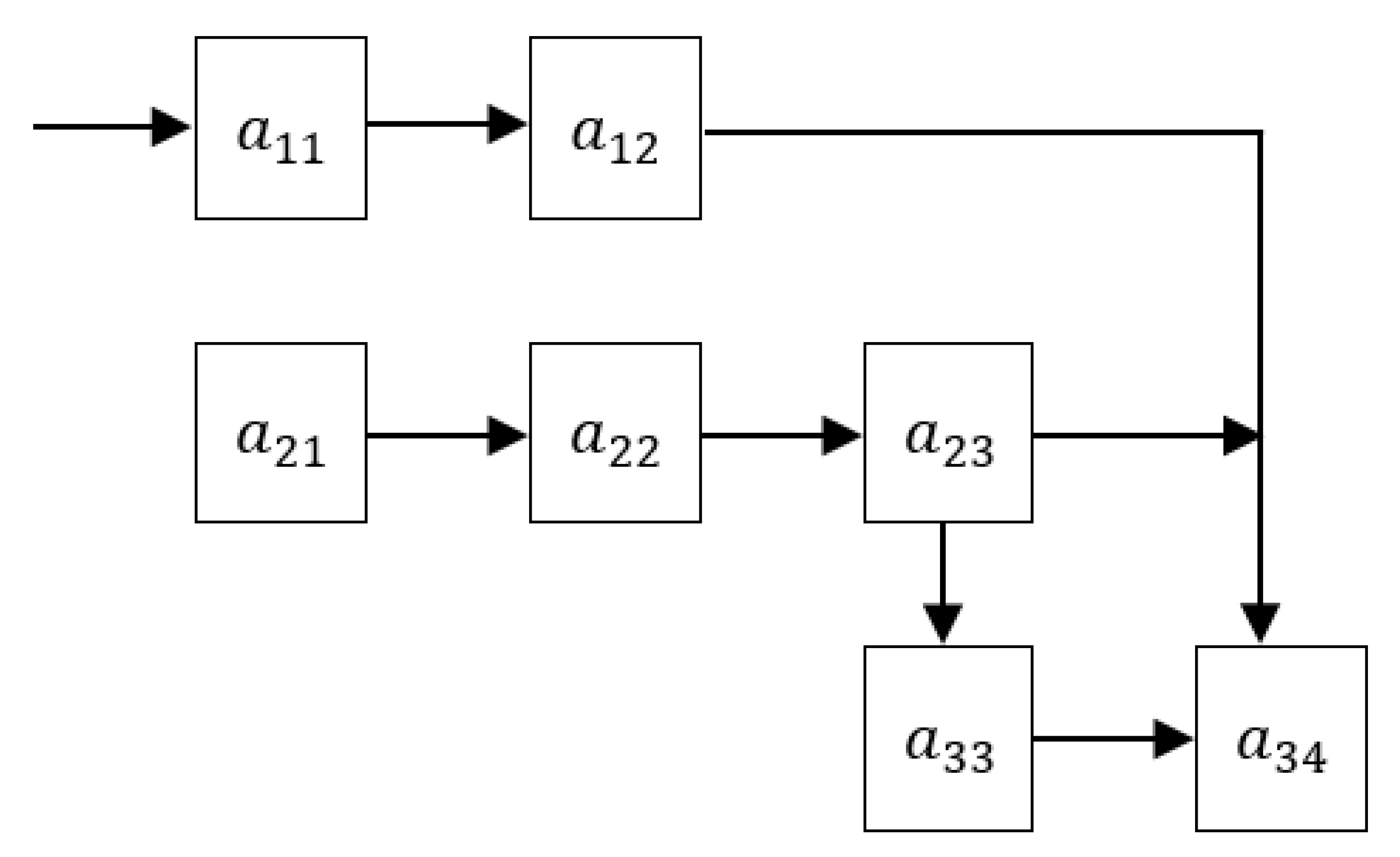
This study initially considers a traditional assembly line that has four workstations with outputs ${\lambda }_A$, ${\lambda }_B$, ${\lambda }_C$, and ${\lambda }_D$ (Figure 1). Thus, the production rate, or output rate, of this assembly line is equal to ${\lambda }_{line}=min.\left\{{\lambda }_A,{\lambda }_B,{\lambda }_C,{\lambda }_D\right\}$.

The cycle time (CT) refers to the longest period required for workstations to complete operations. Therefore, all station operation times are less than or equal to the CT. The aim of balancing the assembly line is to ensure that the output rate and operating time of each workstation are identical. Previous studies have examined assembly line balancing. According to Bartholdi and Eisenstein [11], the assembly line balances itself. They found that if workers are sequenced from slowest to fastest, a stable partition of work spontaneously emerges independent of the stations at which the workers begin. Moreover, the production rate converges to a value. Huang [12] determined that the CT and labor efficiency are negatively exponential to the number of assigned workers. Sawik [13] presented new mixed integer programming formulations for scheduling a flexible flow line with blocking. In this flexible flow line, each stage has one or more identical parallel machines. This study uses parallel operators instead of parallel machines. Rearranging operators may increase the production rate. Muth [14] examined whether a rearrangement in the order of servers affects the production rate. Muth speculated that the production rate remains invariant if the production line is reversed.

If the number of workers at a workstation is more than the number of machines, the machines are expected to limit the output rate and cause a bottleneck. However, Zavadlav et al. [15] showed that the workers, rather than the machines, limit the rate of output.

The manager of a factory always works under “cost” pressure; the company wants the manager to make continual improvements without increasing the cost. Managers typically try to increase the output by adding machines and workers, but managers must first consider whether assembly lines are balanced. When assembly lines are not balanced, productivity is low and workers complain. Workers might not only complain that they have to do more work at their station for the same pay, but also that their skills are not suited to their workstation. This work environment might lead workers to miss shifts on purpose or to resign.

Many ALBP methods have been examined in the study of manufacturing systems, including the heuristic algorithm [16,17,18,19,20,21,22,23,24], artificial bee colony algorithm [25,26,27], genetic algorithm [28,29,30], branch-and-bound algorithm [31,32,33,34], imperialist competitive algorithm [35], Pareto Greedy algorithm [36], memetic ant algorithm [37], whale optimization algorithm [38], recursive algorithm [39], fuzzy linear programming [40], swarm algorithm [41,42], simulated annealing algorithm [43], and data envelopment analysis [44]. The genetic algorithm [45,46] and artificial bee colony algorithm [47] have been used to solve the ALBP in remanufacturing systems. However, studies have seldom discussed how to arrange operators and group similarly skilled operators at the same workstation. This paper considers workers, not machines, in determining whether a workstation has the right equipment and machinery for operators to use. To achieve this goal, the study works out a method for rapidly balancing assembly lines by arranging operators among the workstations and uses a robust, cluster algorithm based on the concept of group technology (GT) to form operator skill cells and determine operator families.

2. Problem Statement

Traditionally, when arranging a limited number of operators on an assembly line, a manager begins with one operator per workstation, before adding an operator to the workstation with the lowest output. Step by step, all of the operators are arranged and the output rate can be found.

When a workstation has a lower output rate, the manager typically adds another operator. However, the lower output might be due to the “human” factor; an operator who is trained on many machines might be assigned to a workstation outside of their skill set. For example, if an operator knows how to work an auto-optical inspection machine but is assigned to a workstation with an in-circuit test machine, the station’s output rate will drop because the operator does not have the required skills. Output can also fall when a worker is absent or resigns unexpectedly and the manager fills the vacancy with a random worker who has not been trained to operate that workstation.

Thus, the problem statement of this study is:

Ideal: The maximum output rate is found, all of the workstations have the same output rate, and the number of operators at each workstation can be found, with all operators assigned to a workstation that matches their skill set.

Reality: The arrangement algorithm is step by step, and the maximum output rate cannot be determined until all of the operators have been arranged. Operators can be assigned to unsuitable workstations.

Consequences: The maximum output rate is an unknown that will affect a boss’s decisions, especially before setting up a new plant. An operator who works at an unsuitable workstation might complain, be absent, or quit unexpectedly, causing a lower output rate.

Proposal: An arrangement algorithm with a constant number of operators must consider the maximum output rate and balance the assembly line without any increase in cost. A sorting algorithm must consider the skills required at each workstation and the skill set of each operator.

3. Methodology

A manager adds a worker to a workstation that has a lower output than at other workstations. When the output of another workstation is lower, the manager adds another worker to that workstation. The use of this step-by-step method balances the assembly lines, especially when setting up a new plant.

3.1. Example of Step-by-Step Method

Suppose an assembly line has six workstations, as shown in Figure 2.

In addition, suppose that the terms $t_{11}, t_{12}, t_{22}, t_{13}, t_{14}, \mathrm{and} t_{15}$ are equal to 12, 15, 10, 16, 20, and 8 min, respectively. If one workday comprises 8 h, then the output per operator per day at each workstation, ${\gamma }_{11}$, ${\gamma }_{12}$, ${\gamma }_{22}$, ${\gamma }_{13}$, ${\gamma }_{14}$, and ${\gamma }_{15}$, are 40, 32, 48, 30, 24, and 60, respectively. Suppose that 500 workers are assigned to this assembly line. The workers can be assigned step by step, as follows (

Table 1. Traditional ALB assignment.

	𝑎11	𝑎12	𝑎22	𝑎13	𝑎14	𝑎15
𝑝ij	1	1	1	1	1	1	∑𝑝ij = 6
𝜆ij	40	32	48	30	24	60	𝜆line = 24

).

The term ${\lambda }_{line}$ is limited in workstation $a_{14}$, which is a bottleneck workstation. Thus, this workstation should have one more operator to increase the output rate. The seventh worker is added to workstation $a_{14}$, and the following is obtained (

Table 2. Traditional ALB assignment.

	𝑎11	𝑎12	𝑎22	𝑎13	𝑎14	𝑎15
𝑝ij	1	1	1	1	2	1	∑𝑝ij = 7
𝜆ij	40	32	48	30	48	60	𝜆line = 30

).

The assignment of workers in a step-by-step manner uses considerable time to obtain the following final result (

Table 3. Traditional ALB assignment.

	𝑎11	𝑎12	𝑎22	𝑎13	𝑎14	𝑎15
𝑝ij	74	92	62	99	123	50	∑𝑝ij = 500
𝜆ij	2960	2944	2976	2970	2952	3000	𝜆line = 2944

).

Considerable time was spent and many steps performed to determine the optimal arrangement of operators at the assembly line’s workstations. Although some studies have discussed and tried to solve the ALBP, the question remains: Is there another method for arranging the workers, instead of using the step-by-step method? This paper presents a novel approach for solving this problem.

Almost all workers require training before operating a workstation. Ideally, the operators on an assembly line would have all of the skills required for each workstation, but that would be very costly. Thus, the operators’ skills must be determined so that they can be placed at a workstation that requires their skills. For example, consider an assembly line that has welding and drilling workstations. If operator $\mathsf{\kappa }$ possesses welding skills, assigning operator $\mathsf{\kappa }$ to the welding workstation rather than to the drilling workstation will reduce the training time for the welding workstation.

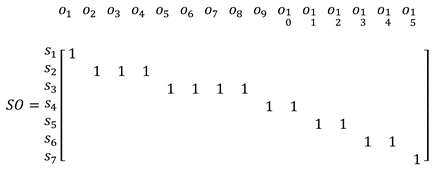
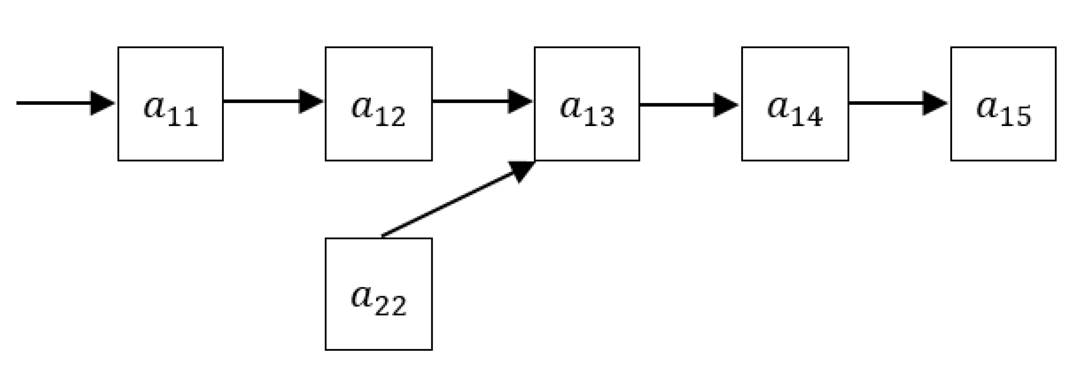
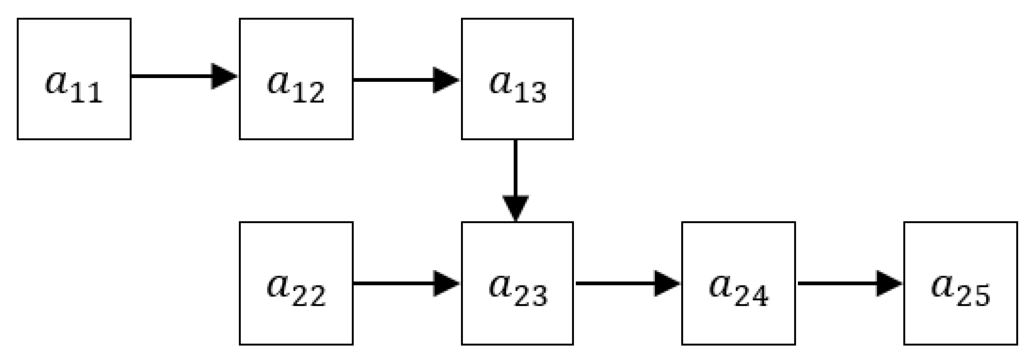
Suppose that there is a balanced assembly line with seven workstations (Figure 3), and workstations 1–7 require one, three, four, two, two, two, and one operator, respectively.

Each workstation requires a skill, which is denoted as $s_1$, $s_2$, ..., $s_7$. A matrix $SO={\left\{s{o}_{ij}\right\}}_{uv}$ describes the relationship between skills and operators. For example, $s{o}_{ij}=1$ indicates that operator $j$ possesses skill $i$. For the assembly line in Figure 3 to function, the minimum matrix $SO$ must be as follows:

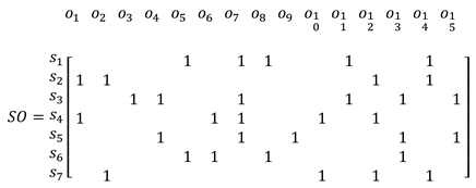
Suppose it is known that:

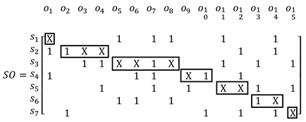
On the basis of the first-come, first-served rule, operator 1 is assigned to $s_1$; operators 2, 3, and 4 are assigned to $s_2$; operators 5, 6, 7, and 8 are assigned to $s_3$; operators 9 and 10 are assigned to $s_4$; operators 11 and 12 are assigned to $s_5$; operators 13 and 14 are assigned to $s_6$; and operator 15 is assigned to $s_7$. Thus, at least 11 operators must take the training course, namely operators 1, 3, 4, 5, 6, 8, 9, 11, 12, 14, and 15, as illustrated in the following matrix where an “X” denotes that the operator needs the training course:

A cluster algorithm is introduced in this paper to reduce the training time and increase the speed at which an assembly line functions. Workers’ absences are also a problem for managers [48,49], but the proposed cluster algorithm can suggest which worker to rotate to a workstation with an absent operator.

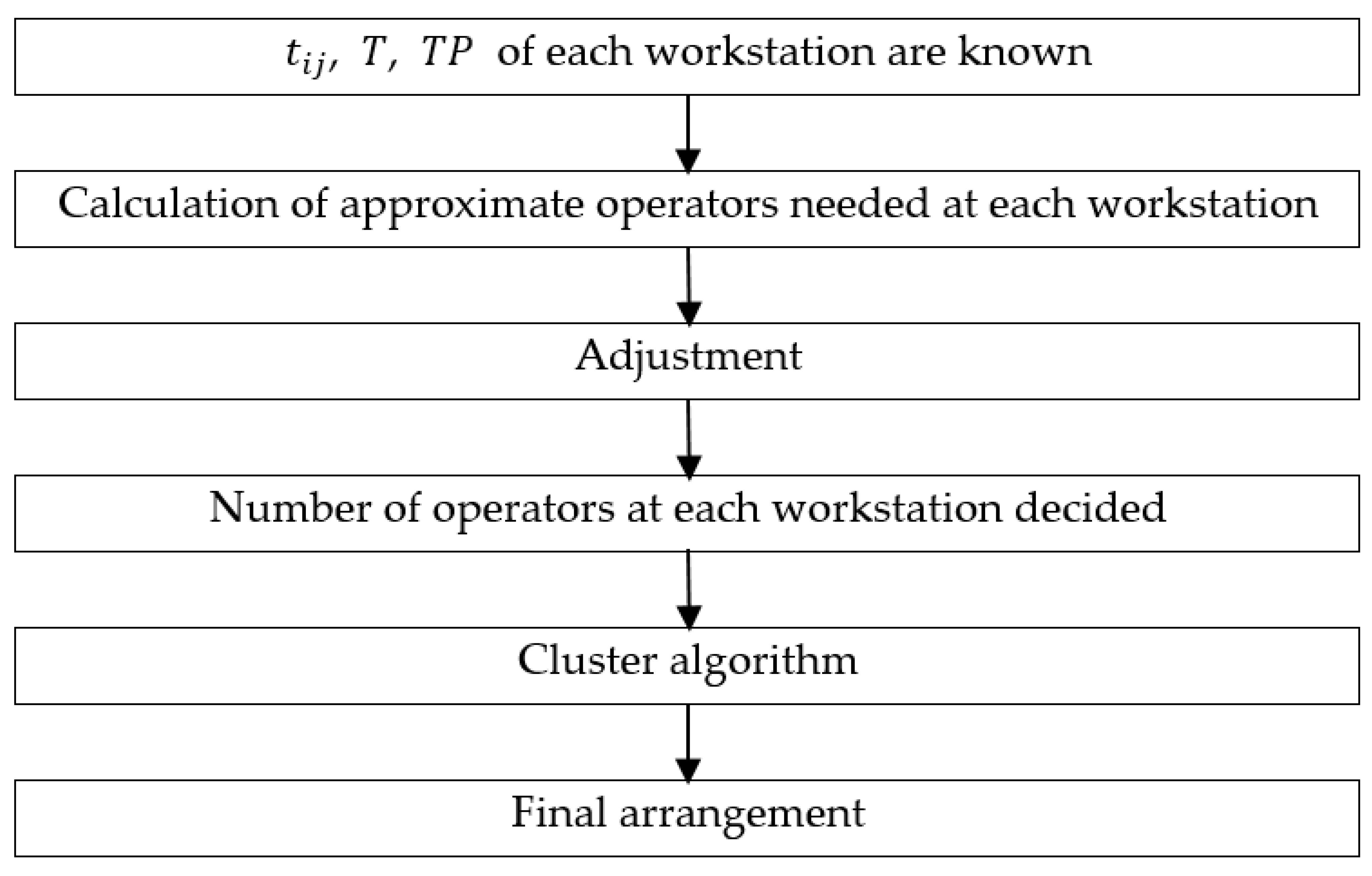
Instead of using the traditional step-by-step method, this study aims to use the proposed algorithm to assign operators to each workstation. Before assigning the operators, some basic data must first be known about each workstation, such as the required skills, the standardization time, the work time per day, and the total number of operators. Then, the approximate number of operators needed at each workstation can be found by using Equations (1)–(7) in Section 3.1. Finally, the number of operators at each workstation can be adjusted by using the traditional step-by-step method. The training time can be reduced by assigning an operator with suitable skills to a suitable workstation, or by sorting the skill–operator matrix by using the cluster algorithm proposed in Section 3.2. The concept is shown in Figure 4.

3.2. Number of Operators at Each Workstation Decided

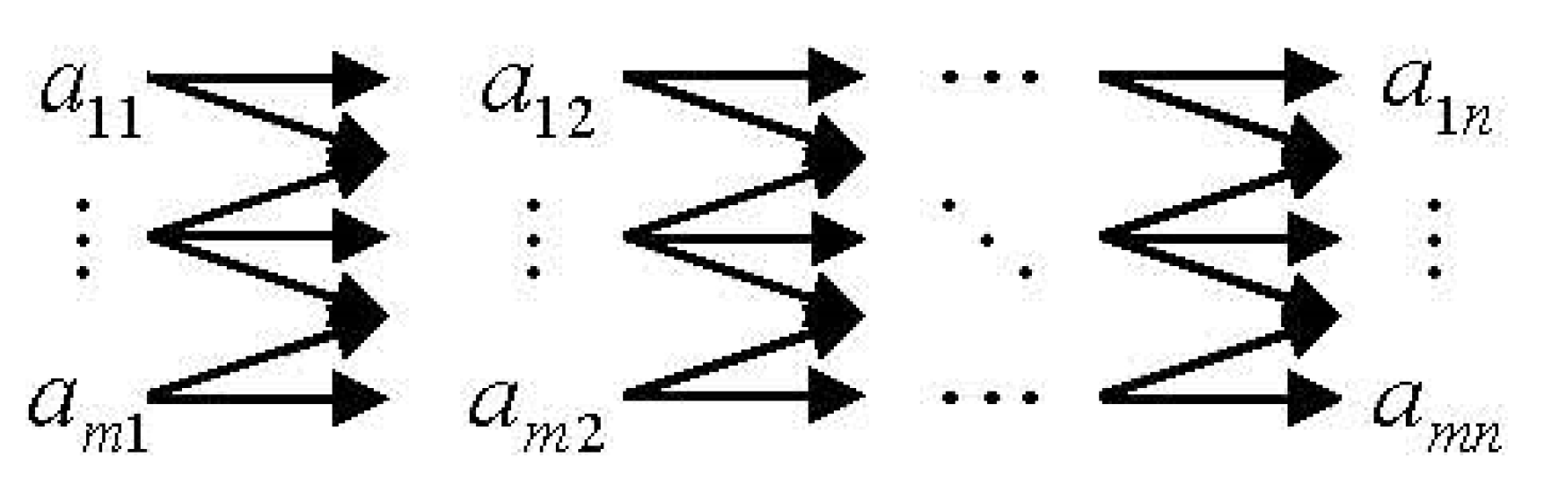
Suppose an assembly line has $m\times n$ workstations (Figure 5).

The matrix $A={\left\{a_{ij}\right\}}_{mn}$ can be used instead of the previous assembly line.

$$A=\left[\begin{array}{c}\begin{array}{cccc}{a}_{11}& a_{12}& \dots & a_{1n}\end{array}\\ \begin{array}{cccc}⋮& ⋮& \ddots & ⋮\end{array}\\ \begin{array}{cccc}{a}_{m1}& a_{m2}& \dots & a_{mn}\end{array}\end{array}\right]$$

The output rate of the assembly line is ${\lambda }_{line}$ where

$${\lambda }_{line}=min.\left\{{\lambda }_{ij}\right\}, 1\le i\le m, 1\le j\le n$$

The ideal assembly line means that

$${\lambda }_{line}={\lambda }_{11}={\lambda }_{21}=\cdots ={\lambda }_{mn}$$

(1)

because

$${\lambda }_{ij}=p_{ij}{\gamma }_{ij}$$

(2)

The term $p_{ij}$ can be easily determined, as follows:

$$p_{ij}=\frac{{\lambda }_{ij}}{{\gamma }_{ij}}$$

(3)

Moreover, the total number of operators is $P$. , where

$$P={\displaystyle \sum }_{i=1}^m{\displaystyle \sum }_{j=1}^n{p}_{ij}$$

(4)

Thus, the following equations are obtained:

$$P={\displaystyle \sum }_{i=1}^m{\displaystyle \sum }_{j=1}^n\frac{{\lambda }_{ij}}{{\gamma }_{ij}}={\lambda }_{line}·{\displaystyle \sum }_{i=1}^m{\displaystyle \sum }_{j=1}^n\frac{1}{{\gamma }_{ij}}={\lambda }_{line}·\frac{1}{T}{\displaystyle \sum }_{i=1}^m{\displaystyle \sum }_{j=1}^n{t}_{ij}$$

(5)

and,

$${\lambda }_{line}=\frac{P}{{{\displaystyle \sum }}_{i=1}^m{{\displaystyle \sum }}_{j=1}^n\frac{1}{{\gamma }_{ij}}}=\frac{P·T}{{{\displaystyle \sum }}_{i=1}^m{{\displaystyle \sum }}_{j=1}^n{t}_{ij}}$$

(6)

Replace ${\lambda }_{ij}$ from Equation (3) with ${\lambda }_{line}$ from Equation (6) to obtain the following equation:

$$p_{ij}=\frac{{\lambda }_{ij}}{{\gamma }_{ij}}=\frac{P}{{\gamma }_{ij}{{\displaystyle \sum }}_{i=1}^m{{\displaystyle \sum }}_{j=1}^n\frac{1}{{\gamma }_{ij}}}=\frac{P·T}{{\gamma }_{ij}{{\displaystyle \sum }}_{i=1}^m{{\displaystyle \sum }}_{j=1}^n{t}_{ij}}$$

(7)

As term $p_{ij}$ is not always an integer, it may need to be chopped off.

Almost all of the operators are now assigned. The traditional step-by-step method is adjusted (as demonstrated in the previous section) and used to assign the remaining workers.

3.3. Cluster Algorithm

The proposed cluster algorithm is based on the concept of GT, which has been applied to cellular manufacturing systems [50,51]. The concept involves grouping machines into machine cells and parts into part families [52,53,54,55,56,57,58,59]. Several algorithms, such as heuristic algorithms [60,61], genetic algorithms [62,63], and neural network algorithms [64], have been derived for solving the GT problem. The proposed algorithm begins with the closeness matrix and a comparison with other algorithms in example 3.

First, the relationship between $u$ skills and $v$ operators, which is represented by the matrix $SO={\left\{s{o}_{ij}\right\}}_{uv}$ is determined as follows:

$$s{o}_{ij}=\{\begin{array}{c}1, if operator j has i skill\\ 0, otherwise\end{array}$$

The closeness matrix of skills is defined as $B_u={\left\{b_{rs}\right\}}_{u\times u}$, where

$$b_{rs}=\{\begin{array}{c}{\displaystyle \sum }_{k=1}^{v}s{o}_{rk}s{o}_{sk}, if r\ne s\\ 0 , otherwise.\end{array}$$

(8)

For example, if there are three workers that know how to operate the welding and milling machines, the closeness between the welding and milling skills is three.

3.3.1. Skills Sorting

Whether two skills are grouped depends on their closeness. Closeness denotes how many operators have both of the skills. The more operators have the two skills, the closer the skills are. First, the skill with the highest closeness value is found and a new group is formed. Second, an unsorted skill follows a sorted skill, based on the highest value in its row in the closeness matrix. If there is no sorted skill to follow, the skill is placed in a new group. Finally, all skills are grouped.

Thus, the skills can be sorted in three steps:

Step 1. Let $f\in G_1$, where $f=\left\{x|b_{xk}=max.\left\{b_{rs}\right\}, 1\le k\le v\right\}$. A tie is broken by selecting the smaller one.

Step 2. Ignore all the grouped rows and form a new closeness matrix $B^{\prime }u=\left\{b_{ij}\right\}$.

Let

$$\{\begin{array}{lll}𝑓\in {𝐺}_k,& & \mathit{if}=\{b_{\mathit{ij}}=\mathit{max}\{b_{\mathit{ij}}\}\mathrm{\wedge }y\in G_k\\ h\in {𝐺}_{\mathit{new}\mathit{group}},& & \mathit{otherwise}\end{array}$$

Step 3. Repeat Step 2 until $u$ skills are grouped.

3.3.2. Operator Sorting

Operator sorting aims to place operators in the group that will use the highest number of their skills.

Thus, let $v\in G_y, y=\left\{x|{\displaystyle \sum }_{u\in G_x}s{o}_{uv}=max.\left({\displaystyle \sum }_{u\in G_i}s{o}_{uv}\right), 1\le i\le R\right\}$. A tie is broken by choosing the group with the lowest number of machines.

3.4. GT Efficiency

This work uses the GT efficiency measurement equation defined by Chandrasekharan and Rajagopalan [65], while letting $q$ be equal to 0.5, as follows:

$$\eta =q{\eta }_1+\left(1-q\right){\eta }_2=q\frac{e_b}{{{\displaystyle \sum }}^{}{Q}_i{P}_i}+\left(1-q\right)\left(1-\frac{e_0}{uv-{{\displaystyle \sum }}^{}{Q}_i{P}_i}\right)$$

(9)

There are two concerns: the “1” in the group, and the “1” not in the group. The higher the GT efficiency, the more 1s are in the groups, and the fewer 1s are not in the groups. Thus, $\frac{e_b}{{{\displaystyle \sum }}^{}N{S}_{i}N{O}_i}$ is the ratio of the number of 1s in the groups to the number of 1s and 0s in all groups, while $\frac{e_0}{uv-{{\displaystyle \sum }}^{}N{S}_{i}N{O}_i}$ is the ratio of the number of 1s not in the groups to the number of 1s and 0s not in the groups.

4. Numerical Examples

4.1. Example 1: Number of Operators at Each Workstation Decided

On an assembly line, 500 operators must be assigned to workstations (Figure 6).

Let

$$A=\left[\begin{array}{ccccc}{a}_{11}& a_{12}& a_{13}& & \\ & a_{22}& a_{23}& a_{24}& a_{25}\end{array}\right]$$

and

$$\left\{t_{ij}\right\}=\left[\begin{array}{ccccc}10& 30& 24& 0& 0\\ 0& 5& 40& 20& 15\end{array}\right]$$

Let the work time per day be 8 h.

Thus,

$$\left\{{\gamma }_{ij}\right\}=\left[\begin{array}{ccccc}48& 16& 20& 0& 0\\ 0& 96& 12& 24& 32\end{array}\right]$$

Thus, from Equation (6), ${\lambda }_{line}=5000/3$, and from Equation (8),

$$\left\{p_{ij}\right\}\begin{array}{c}chop off\\ ~\end{array}\left[\begin{array}{ccccc}34& 104& 83& & \\ & 17& 138& 69& 52\end{array}\right]$$

The approximate operators needed at each workstation are as follows (

Table 4. Approximate operators needed at each workstation.

	𝑎11	𝑎12	𝑎13	𝑎22	𝑎23	𝑎24	𝑎25
𝑝ij	34	104	83	17	138	69	52	∑𝑝ij = 497
𝜆ij	1632	1664	1660	1632	1656	1656	1664	𝜆line = 1632

).

The traditional step-by-step method is adjusted to obtain

Table 5. Final ALB solution proposed by this study.

	𝑎11	𝑎12	𝑎13	𝑎22	𝑎23	𝑎24	𝑎25
𝑝ij	35	104	83	18	138	69	52	∑𝑝ij = 499
𝜆ij	1680	1664	1660	1728	1656	1656	1664	𝜆line = 1656

. Stations $a_{11}$ and $a_{22}$ are the bottleneck stations. Thus, if only one worker is assigned (the 498th one) to station $a_{11}$ or station $a_{22}$, the assembly line cannot function. The production rate is increased if another worker is assigned to station $a_{11}$ and another is assigned to station $a_{22}$. The final ALB solution is as follows (Table 5).

4.2. Example 2: Auditing Production Rate

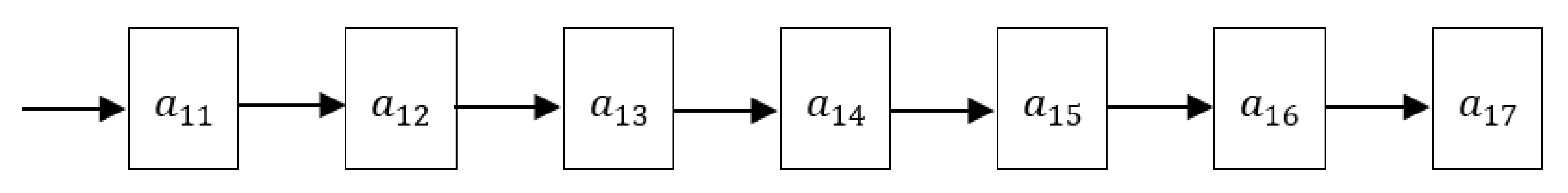
The proposed method can be used to audit the production rate, which could be increased by rearranging the operators at each station. Consider this numerical example: An assembly line has seven workstations and 1100 workers (Figure 7).

Let

$$A=\left[\begin{array}{cccc}{a}_{11}& a_{12}& & \\ a_{21}& a_{22}& a_{23}& \\ & & a_{33}& a_{34}\end{array}\right]$$

$$\left\{t_{ij}\right\}=\left[\begin{array}{cccc}10& 30& & \\ 20& 40& 15& \\ & & 24& 48\end{array}\right]$$

and

$$\left\{p_{ij}\right\}=\left[\begin{array}{cccc}70& 180& & \\ 120& 200& 80& \\ & & 150& 300\end{array}\right]$$

Let the work hours per day be 8 h. Thus, the following matrix is obtained:

$$\left\{{\gamma }_{ij}\right\}=\left[\begin{array}{cccc}48& 16& & \\ 24& 12& 32& \\ & & 20& 10\end{array}\right]$$

From Equation (2), the following matrix is obtained:

$$\left\{{\lambda }_{ij}\right\}=\left[\begin{array}{cccc}3360& 2880& & \\ 2880& 2400& 2560& \\ & & 3000& 3000\end{array}\right]$$

where ${\lambda }_{line}$ = 2400. If the workers are rearranged, the output rate is increased without any increase in cost. Equation (6) is used in the method proposed in this study: ${\lambda }_{line}$ = 528,000/187. Thus, the following matrix is obtained:

The traditional step-by-step method is adjusted to derive the final arrangement (

Table 6. Final ALB solution proposed by this study.

	𝑎11	𝑎12	𝑎21	𝑎22	𝑎23	𝑎33	𝑎34
𝑝ij	59	176	118	235	88	141	282	∑𝑝ij = 1099
𝜆ij	2832	2816	2832	2820	2816	2820	2820	𝜆line = 2816

):

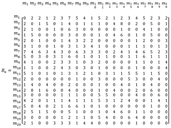
4.3. Example 3: Comparison with Boe and Cheng’s Algorithm

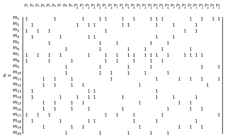
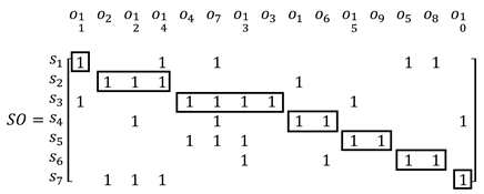
This example compares the proposed algorithm with Boe and Cheng’s close neighbor algorithm [66]. The original part–machine incidence matrix is taken from Boe and Cheng as follows:

4.3.1. Machine Sorting

First, the relationship between the two machines must be obtained. For example, Equation (8) is used to obtain $b_{37}$.

$$b_{37}=1\times 1+0\times 0+1\times 1+\dots +0\times 0=6$$

Thus, the closeness matrix of skills is as follows.

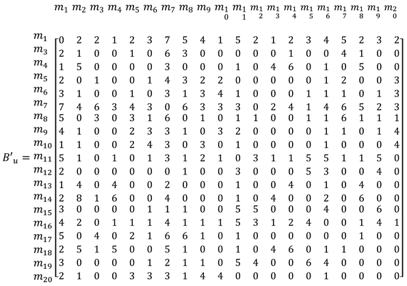
In step 1 of machine sorting, the first machine, belonging to the first group, is $m_2$. Thus, $G_1=\left\{m_2\right\}$. Ignoring $m_2$, the next step is to form a new closeness matrix of skill $B^{\prime }u=\left\{b_{kl}\right\}$, as follows:

The next machine is $m_{14}$, which belongs to $G_1$ because $b_{m_{14}{m}_2}$ is the largest number in $B^{\prime }u$. Thus, $G_1=\left\{m_2, m_{14}\right\}$. The new closeness matrix of skill $B^{\prime }u=\left\{b_{kl}\right\}$ is as follows:

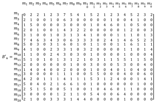
The third machine is $m_1$, which belongs to a new group, $G_2$, because $b_{m_1{m}_7}$ is the largest number in $B^{\prime }u$, but machine $m_7$ does not belong to any group. Thus, $G_2=\left\{m_1\right\}$. Applying steps 2–3 in Section 3.3.1 gives four groups: $G_1=\left\{m_2, m_{14}, m_4, m_{18}, m_{13} \right\}$, $G_2=\left\{m_1, m_7, m_3, m_8, m_{17}, m_5, m_9\right\}$, $G_3=\left\{m_{15}, m_{19}, m_{11}, m_{12}, m_{16} \right\}$, and $G_4=\left\{m_6, m_{10}, m_{20}\right\}$.

4.3.2. Part Sorting

By using the operator sorting step in Section 3.3.2, the parts can be sorted. For example, $p_{24}$, the ${\displaystyle \sum }_{u\in G_1}s{o}_{u{p}_{24}}=5$, and 2, 1, and 0 in $G_2$, $G_3$, and $G_4$, respectively. Thus, $p_{24}$ belongs to $G_1$.

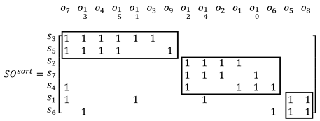
Finally, the four groups are ordered (

Table 7. The four groups in example 3.

Groups	Group Members
G1	m2,m14,m4,m18,m13,p2,p7,p10,p12,p13,p18,p24,p27,p31
G2	m1,m7,m3,m8,m17,m5,m9,p1,p3,p5,p15,p17,p20,p23,p25,p29,p34,p35
G3	m15,m19,m11,m12,m16,p4,p6,p9,p11,p21,p28,p30,p32,p33
G4	m6,m10,m20,p8,p14,p16,p19,p22,p26,

).

The sorted incidence matrix is as follows:

Boe and Cheng’s solution of this example is as follows:

The GT efficiency of the proposed algorithm is obtained using Equation (9), as follows:

$$\eta =0.5\times \frac{33+40+31+14}{5\times 9+7\times 11+5\times 9+3\times 6}+0.5\times \left(1-\frac{35}{20\times 35-\left(5\times 9+7\times 11+5\times 9+3\times 6\right)}\right)=78.5\%$$

In the same way, GT efficiency is calculated using Boe and Cheng’s algorithm, as follows:

$$\eta =0.5\times \frac{40+18+33+22}{7\times 11+3\times 8+5\times 9+5\times 7}+0.5\times \left(1-\frac{40}{20\times 35-\left(7\times 11+3\times 8+5\times 9+5\times 7\right)}\right)=77.4\%$$

4.4. Example 4: Reducing Training Time

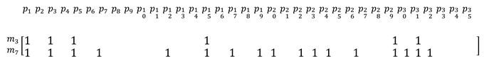
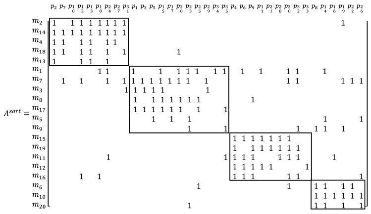
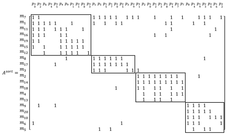
This example demonstrates how to find an operator with the training and skills that matches a workstation’s skill requirements so that the operator does not need to take any training courses. Consider the problem displayed in Figure 3 (Section 2). The proposed algorithm is used to obtain a sorted skill-operator matrix, as follows:

A manager could use the sorted skill–operator matrix as a database for choosing an operator with the right training and skills. Based on the database, the manager could quickly rotate a suitable worker to a workstation. Based on the sorted skill–operator matrix $S{O}^{sort}$, the manager could choose operator $o_{11}$ for the workstation that requires skill $s_1$; $o_2$, $o_{12}$, and $o_{14}$ because of $s_2$; $o_4$, $o_7$, $o_{13}$, and $o_3$, because of $s_3$; $o_1$ and $o_6$ because of $s_4$; $o_{15}$ and $o_9$ because of $s_5$; $o_5$ and $o_8$ because of $s_6$; and $o_{10}$ because of $s_7$, as follows:

Operators in the same skills group can support other operators in the group.

5. Results and Discussion

In example 1, stations $a_{23}$ and $a_{24}$ are the bottleneck stations. However, only one operator, namely the 500th one, can be assigned. Assigning the 500th operator to either station $a_{23}$ or $a_{24}$ cannot increase the output of the assembly line. This study suggests that the 500th worker should be laid off or shifted to another department. Alternatively, a 501st operator could be hired, which would allow another worker to be assigned to station $a_{23}$ and another to be assigned to station $a_{24}$. This example demonstrates the proposed method in detail. The maximum output rate and the number of workers at each workstation can be decided. It also shows that multiple workstations can simultaneously become bottleneck stations.

In example 2, stations $a_{12}$ and $a_{23}$ are the bottleneck stations, and only one operator can be assigned. This study suggests that the 1100th worker be laid off or shifted to another department. Alternatively, a 1101st operator could be hired, which would allow another worker to be assigned to station $a_{12}$ and another to be assigned to station $a_{23}$. With these solutions, a higher production rate than in the original arrangement (2816 > 2400) is achieved without any increase in cost. It shows that a manager can improve productivity by rearranging the number of workers at each workstation, while not increasing costs. It will also cut down on worker complaints because the workers’ workloads are balanced.

In example 3, the proposed algorithm is used to categorize four groups, as shown in Section 4.3. Boe and Cheng‘s algorithm is compared with the GT efficiency measure proposed by Chandrasekharan and Rajagopalan. The GT efficiency of the proposed algorithm is 78.5%, higher than the 77.4% of Boe and Cheng‘s algorithm. Thus, the proposed GT algorithm works and can perform better than other algorithms in the literature. Workers are assigned to the workstation that best uses their skills, so they feel that their contribution is meaningful and more substantial. Workers at the same workstation also share more skills in common. This makes it easier for the manager to alternate workers.

In example 4, operators within the same skill group can support each other, giving managers more worker rotation solutions. With workers suggested by the sorted skill–operator matrix, managers can quickly match suitable operators with workstations so that productivity remains high. Using the matrix to match workers’ training and skills to workstations’ skill requirements also enables managers to reduce operator training time and cover workers’ absences. For example, if $o_4$ is absent or busy, then $o_{15}$ can support or share the workload without needing too much training. The risk of an unexpected worker absence or resignation can be mitigated by alternating the workers according to the sorted skill–operator matrix.

6. Conclusions

Company managers aim to achieve sustainable operations, part of which is managing labor costs. To reduce labor costs, an assembly line manager increases the line’s efficiency and reduces the training time needed by operators. Inadequate training or distractions, such as an operator focused on a personal problem, can be dangerous, something a plant manager seeks to eliminate, while worker absences hurt efficiency and increase costs. This paper presents an algorithm that helps managers keep assembly lines balanced by arranging operators, so a line’s workstations achieve the same output rates. The first example demonstrates how the proposed method can decide the maximum output rate and the number of workers at each workstation given a constant number of operators, especially when setting up a new plant. The second example demonstrates how the method can audit the existing number of operators at each workstation. Using the method to readjust the number of operators at a workstation can increase the output rate, without raising costs. As indicated in the numerical examples, another challenge is that multiple workstations can simultaneously become bottleneck stations. Knowing the number of operators at each workstation, the proposed cluster algorithm can group operators with similar skills and training, which reduces the training time. The third example demonstrates how the proposed clustering algorithm performs better than a previously described algorithm. Within the same group, operators from one workstation can also support operators at other workstations, as demonstrated in example 4. The clustering algorithm could be used by the human resources department to make a database that includes all of the company employees. When an employee is absent, a manger could quickly find a replacement, mitigating the risk of an unexpected absence. The manager could also use such a database to determine which employees should take a training course. By not having all of the employees take the training course, training costs could be reduced. Future applications of the proposed method could include the creation of a course-faculty database, where it could be used to find a replacement instructor for a class when the assigned instructor is absent.

Traditional GT considers only machines and parts, but this study uses the concept of GT to reduce the training time of workstation operators so that managers can achieve sustainable operations. The sorted skill–operator matrix in this study can, similar to a database, provide a manager with suggestions. However, most managers prefer a direct solution to a problem; they want the specific worker whose training and skills match the skill requirements of the problem workstation. Thus, future studies could develop an algorithm to assign specific workers to specific workstations by using a sorted skill–operator matrix, especially for large factories with multiple assembly lines.