Measuring Ocean Surface Current in the Kuroshio Region Using Gaofen-3 SAR Data

Abstract

The Kuroshio is the strongest warm current in the western North Pacific, which plays a crucial role in climate and human activities. In terms of this, the accurate acquisition of ocean surface current velocity and direction in the Kuroshio region is of great research value. Gaofen-3 synthetic aperture radar (SAR) provides data support for the study of ocean surface current measurements in the Kuroshio region, but no relevant experimental result has been published yet. In this paper, four available stripmap mode SARs’ data acquired by Gaofen-3 in the Kuroshio region are used for measuring the ocean surface current field. In general, the Doppler centroid anomaly (DCA) estimation is a common method to infer ocean surface currents from single-antenna stripmap data, but only the radial velocity component can be retrieved. In order to measure current vectors, a novel method combining the sub-aperture processing and the least squares (LS) technology is suggested and demonstrated by applying to the Gaofen-3 SAR data processing. The experiment’s results agree well with model-derived ocean current data, indicating that the Gaofen-3 SAR has the capability to accurately retrieve the ocean surface current field in the Kuroshio region and motivate further research by providing more data.

1. Introduction

Current is ubiquitous in the global ocean, the information about which is valuable in many applications. The circulation current in different regions of the deep ocean will exchange material and energy, which is of great importance for the global climate process. Moreover, monitoring currents in the coastal waters is conducive to navigation, offshore oil and gas field development, fishery resources management, and so forth. According to the data requirements survey report on oceanic variables issued by EuroGOOS, the ocean surface current velocity and direction were the two most requested [1]. Therefore, it is necessary to investigate various methods for measuring the velocity and direction values of the ocean current field. Compared with the in-situ current measurement tools, such as drift buoy and current meter, which are time-consuming and limited in spatial measurement range, the spaceborne synthetic aperture radar (SAR) has become a vital tool for ocean remote sensing mainly due to its day/night and quasi-all-weather capability and its high-spatial resolution [2].

There are two common techniques used for current measurement with SAR data, that is, one is Doppler centroid analysis (DCA) and the other is along-track interferometry (ATI) [3,4]. DCA is suitable for single-antenna SAR data processing and has low requirements for the system. Chapron [5] first proposed the DCA method in 2005 and processed the ENVISAT ASAR data to retrieve the radial velocity of the sea surface in different areas including the current field near the Gulf Stream. In the following years, the DCA method was used many times to measure the ocean surface current field in the Agulhas Current regime [6,7,8]. These studies show that DCA has good applications in these regions with strong boundary currents. The Kuroshio Current is also one of the strongest western boundary currents, but there have not yet been any relevant SAR experimental results applied to the Kuroshio region. In addition, the DCA method using Doppler centroid shift can only derive the line-of sight (LOS) velocity component of ocean surface current, not including the direction values. The ATI method uses interferometric phase to achieve high-resolution ocean surface current measurements. Moreover, ATI systems can be transformed into ones with squint beams to measure the ocean current vectors [9,10,11]. However, ATI needs to operate the SAR data of at least two antennas; the related system is complicated, the experimental data are small, and it is far from scale application than DCA using single SAR data.

Like the Gulf Stream in the North Atlantic, the Kuroshio is a powerful western boundary current and forms the western limb of the North Pacific Subtropical Gyre. Owing to the influence of the geostrophic Coriolis force, the remote sensing measurement of Kuroshio current speed can be performed with the spaceborne altimeters [12,13], but the spatial resolution is relatively rough, reaching tens of kilometers, and the data around the land are easily missed. Gaofen-3 is China’s first C-band full-polarization synthetic aperture radar imaging satellite, which provides reliable high-resolution SAR image data for ocean remote sensing [14]. So far, Gaofen-3 SAR data have been used to study ocean surface waves [15], ocean winds [16] and internal waves [17]. Gaofen-3 provides data support for the ocean current retrieval in the Kuroshio region, which will promote relevant application research.

This paper uses four available Gaofen-3 SAR datasets to measure the ocean surface current in the Kuroshio region. In order to retrieve current velocity and direction information at the same time, a novel method combining sub-aperture processing technology and least squares technology is proposed and applied. The following second part introduces the principle and process of the data processing method in detail. The third part is to carry out the ocean current measurement experiment of the Gaofen-3 SAR data and verify the experimental results. The fourth part discusses and analyzes the applicability of the method, including the influence of system and environmental factors on the results, and the fifth part presents conclusions.

2. Measurement of the Ocean Surface Current

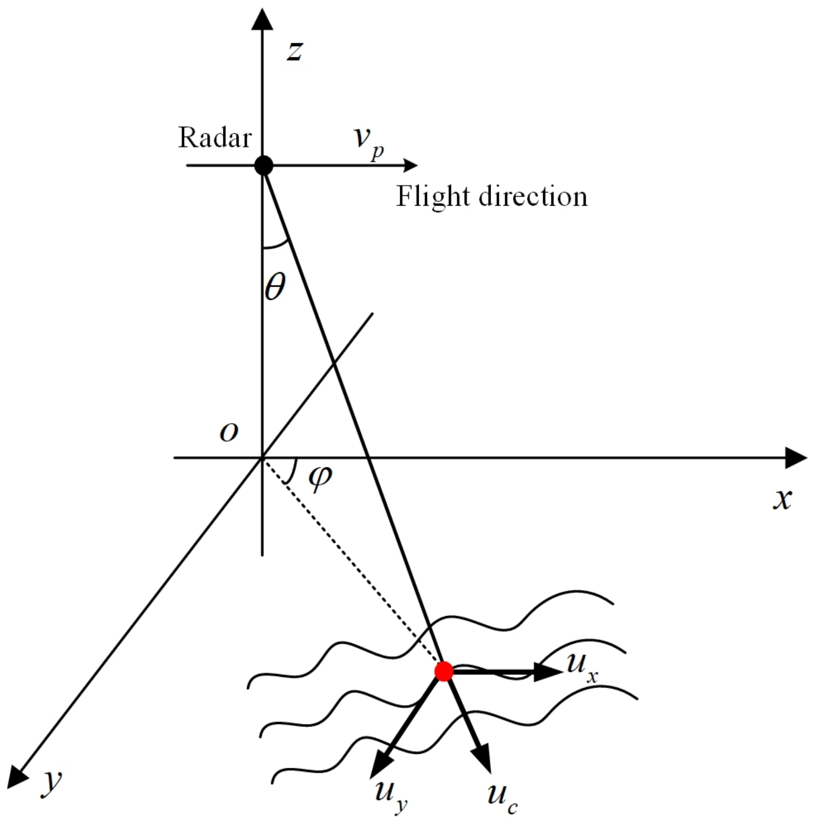
2.1. Ocean Doppler Information of Single Antenna SAR Data

Due to the relative motion between the SAR platform and the ocean surface, the azimuth Doppler information of the echo signal would change, suggesting that the Doppler frequency can be used to retrieve the ocean surface motion. In fact, considering the complexity of ocean motion and the particularity of SAR for ocean imaging, the estimated Doppler centroid shift in SAR ocean data usually includes the following items [18]:

$$f_{dc}=f_{dc}^{phys}+f_{dc}^{geo}+f_{dc}^{ele}+▵f_{dc}.$$

(1)

In Equation (1), $f_{dc}^{phys}$ is the geophysical term, $f_{dc}^{geo}$ is the geometric attitude term, $f_{dc}^{ele}$ indicates electronic misdirection of antenna, $▵f_{dc}$ represents the residual error in data processing. As one of our concerns, $f_{dc}^{phys}$ is proportional to the ocean surface Doppler velocity in the line-of-sight direction, which contains not only the information of ocean currents, but also the contributions of wind and wave motion. In Bragg theory, wind and wave motion primarily involve Bragg wave phase velocity and large-scale wave orbit velocity. Therefore, $f_{dc}^{phys}$ can be expressed as

$$f_{dc}^{phys}=f_c+f_b+f_o,$$

(2)

where $f_c$, $f_b$ and $f_o$ denote the Doppler centroid frequency variation caused by ocean currents, Bragg wave phase velocity, and large-scale wave orbit velocity, respectively. How to estimate $f_{dc}^{phys}$ from $f_{dc}$ has been studied in detail in reference [8], and the relevant data processing process will not be discussed. The focus of this paper is to separate $f_c$ from $f_{dc}^{phys}$ and further extract the ocean current information.

According to the geometric relationship between ocean current and SAR platform shown in Figure 1, $f_c$ can be expressed as:

$$f_c=\frac{2}{\lambda }(u_{x}cos\phi sin\theta +u_{y}sin\phi sin\theta ),$$

(3)

where $u_x$ and $u_y$ represent the azimuth and range velocity components of the current, respectively. $\phi$ is the angle between the beam center and the flight direction in the horizontal plane, which is called the azimuth angle. $\theta$ is the incidence angle, and $\lambda$ is the electromagnetic wavelength. We can also obtain the Doppler frequency caused by platform movement as:

$$f_p=\frac{2v_p}{\lambda }cos\phi sin\theta ,$$

(4)

where $v_p$ is the radar speed.

In Bragg scattering theory, Bragg resonance is the main SAR imaging mechanism for the ocean surface. Furthermore, the phase velocity of the Bragg wave is the main factor affecting the deviation of current measurements, which is expressed as [19,20]:

$$c=\sqrt{g/k_b+T{k}_b},$$

(5)

where g is the acceleration of gravity, and T is the ratio of water surface tension to seawater density. $k_b=2\pi /{\lambda }_b$ is the wavenumber of Bragg waves, which can be expressed by electromagnetic wavenumber $k_e$ and incidence angle ${\theta }_e$ as

$$k_b=2k_{e}sin{\theta }_e.$$

(6)

Therefore, the Doppler centroid variation caused by the Bragg wave phase velocity is

$$f_b=\frac{2}{\lambda }\sqrt{g/k_b+T{k}_b}.$$

(7)

In the composite surface model, as one form of Bragg theory, there are not only small-scale Bragg waves but also large-scale modulating waves on the ocean surface. In this situation, the large-scale waves will be displayed in SAR images by modulating the energy distribution of Bragg waves, and the Doppler centroid will also shift with the variation of large-scale wave orbital velocity, that is, there is $f_o$, which also results in the deviation of current measurements. Generally, the orbital velocity is affected by the weighted average of the local backscatter within the SAR resolution cell and during the SAR integration time [4,5]. In some studies [4,21,22], the empirical model derived from actual data fitting can be used to remove the motion induced by wind and waves, including the effect of orbital speed. This processing method is in good agreement with the actual situation, but is limited by different sensor data and sea surface position, the measurement accuracy will be different. Yu et al. [23] also pointed out that the influence of orbital velocity can be suppressed by space averaging. This operation is simple, but the residual error will be left.

Motion errors will affect SAR imaging and sea surface current field estimation. Reference [24] states that motion errors decrease the image quality in the course of imaging. In principle, the uncertainty caused by motion errors can be corrected with the motion measurement data obtained from the global positioning system (GPS) or other ancillary instrument. In Reference [24], a deep SAR motion compensation scheme is proposed to be combined with the deep SAR imaging algorithm, which could eliminate the influence of motion errors and improve SAR imagery quality in practical applications. Reference [25] also discusses the influence of motion errors on imaging, and points out that classical motion compensation is typically not required for spaceborne systems due to their stable and homogeneous motion. The Gaofen-3 satellite adopts a dual frequency GPS system to realize precise orbit determination, which has high attitude control accuracy and stability [26]. Therefore, the motion errors have a limited impact on the imaging results.

For the application of current measurements, the influence of motion and attitude errors on the predicted Doppler shift is mainly considered, as shown in Reference [8]. Due to errors in satellite position and attitude used to predict the Doppler shift, the ocean current product will deviate. After attitude control, the Gaofen-3 satellite eliminates the change of Doppler center frequency caused by earth rotation, earth ellipticity and satellite orbit oblateness [26]. Therefore, the predicted Doppler shift of SAR data is close to zero. If the azimuth angle error $▵\phi$ is considered in current measurements with actual data, the Doppler frequency caused by platform motion will have errors [27]. Therefore, Equation (8) can be obtained based on Equation (4), and the Doppler frequency caused by current becomes Equation (9):

$$\begin{array}{cc}\hfill ▵f_a& =\frac{2v_p}{\lambda }[cos(\phi +▵\phi )sin\theta -cos\phi sin\theta ]\hfill \\ & \approx -\frac{2}{\lambda }{v}_p▵\phi sin\phi sin\theta \hfill \end{array}$$

(8)

$$\begin{array}{cc}\hfill f_c^{{}^{\prime }}& =\frac{2sin\theta }{\lambda }\left[u_{x}cos\left(\phi +\Delta \phi \right)+u_{y}sin\left(\phi +\Delta \phi \right)\right]\hfill \\ & \approx \frac{2sin\theta }{\lambda }\left[\left(u_x+\Delta \phi u_y\right)cos\phi +\left(u_y-\Delta \phi u_x\right)sin\phi \right].\hfill \end{array}$$

(9)

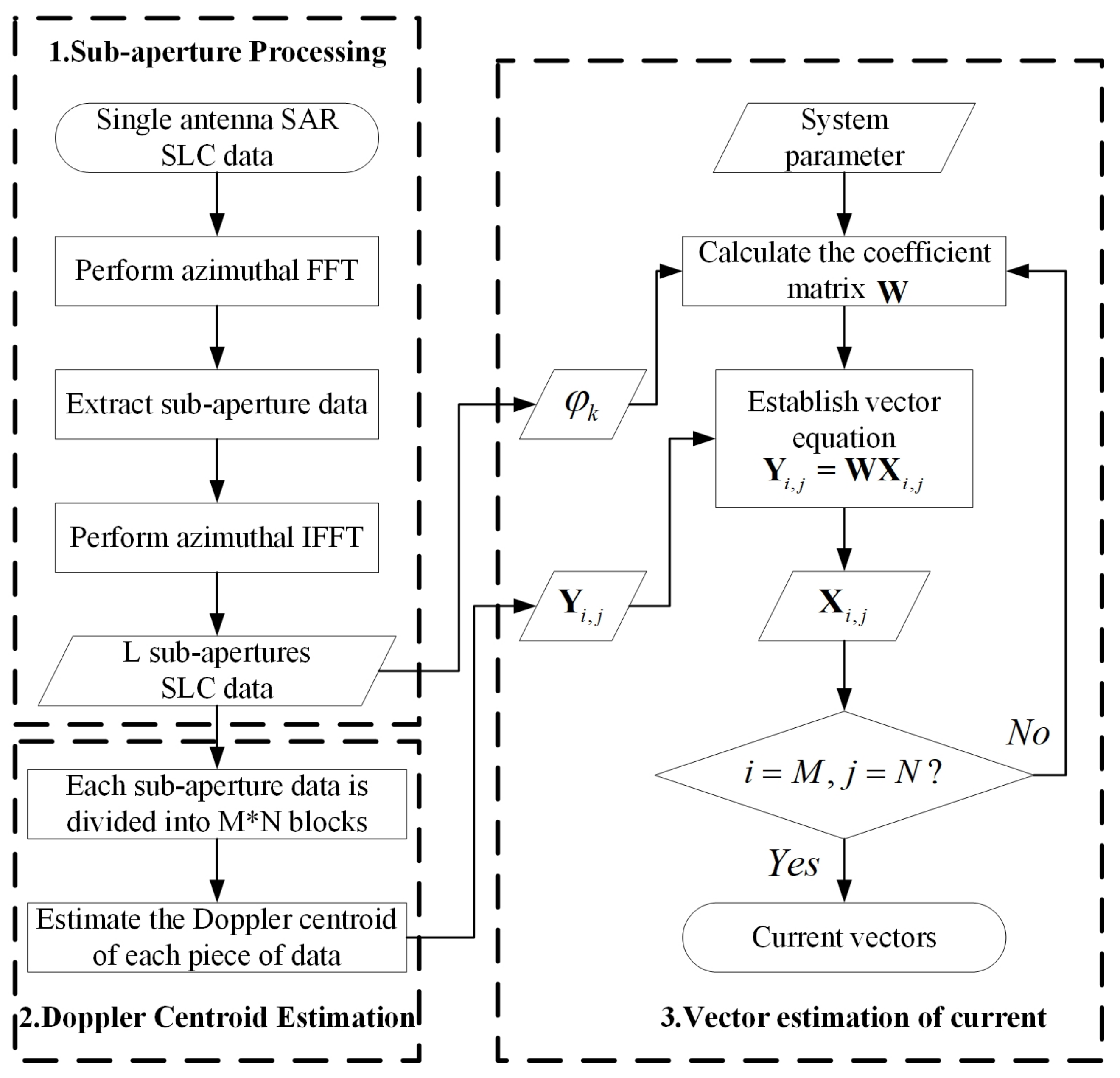
2.2. Measurement Method with Single Antenna SAR Data

According to the above analysis, the Doppler centroids in different azimuth angles reflect the current information in different directions. However, single antenna full-aperture SAR data usually only provide the Doppler frequency in one direction. Therefore, the method in this paper firstly carries out sub-aperture processing to acquire sub-apertures image data representing different look directions, and then carries out Doppler centroid estimation, respectively. Furthermore, the equations are established according to the estimated Doppler centroids. Finally, the current vectors are estimated by the least squares method. This method can be divided into three steps: sub-aperture processing, Doppler centroid estimation and vector estimation of current. The flow chart is shown in Figure 2.

In the first step, the input is Gaofen-3 single look complex (SLC) data. After implementing azimuth FFT of the input SLC, the sub-aperture data is extracted by aperture division in the Doppler frequency domain, then IFFT is performed to acquire L sub-aperture SLC in time-domain as the output of the first step. Besides, the azimuth angle ${\phi }_k$ corresponding to each sub-aperture is also the output and used as the input for the third step. The L sub-aperture SLC is inputted in step 2 to estimate the Doppler frequency of each sub-aperture, respectively. In step 2, each input sub-aperture SLC data is divided into $M*N$ blocks, and the Doppler centroid frequency of each block is estimated. The Doppler frequency at the same spatial position block $(i,j)$ with different sub-apertures form a vector ${\mathbf{Y}}_{i,j}$ as the output. Therefore, azimuth angle ${\phi }_k$ and vector ${\mathbf{Y}}_{i,j}$ are the inputs of the third part. The coefficient matrix $\mathbf{W}$ is generated by combining the Gaofen-3 system parameters, that is, wavelength, incident angle, flight speed, and the azimuth angle of L sub-apertures. Then, the vector equation of the unknown vector $\mathbf{X}$ is established with vectors ${\mathbf{Y}}_{i,j}$ and $\mathbf{W}$. The unknown vector $\mathbf{X}$ includes current vector information, so the current vector at each position in space can be calculated by solving the equation with the least squares method. The output of step 3 is the sea surface current field of the entire data. The specific processing process and the calculation of variables are explained respectively in the following subsection.

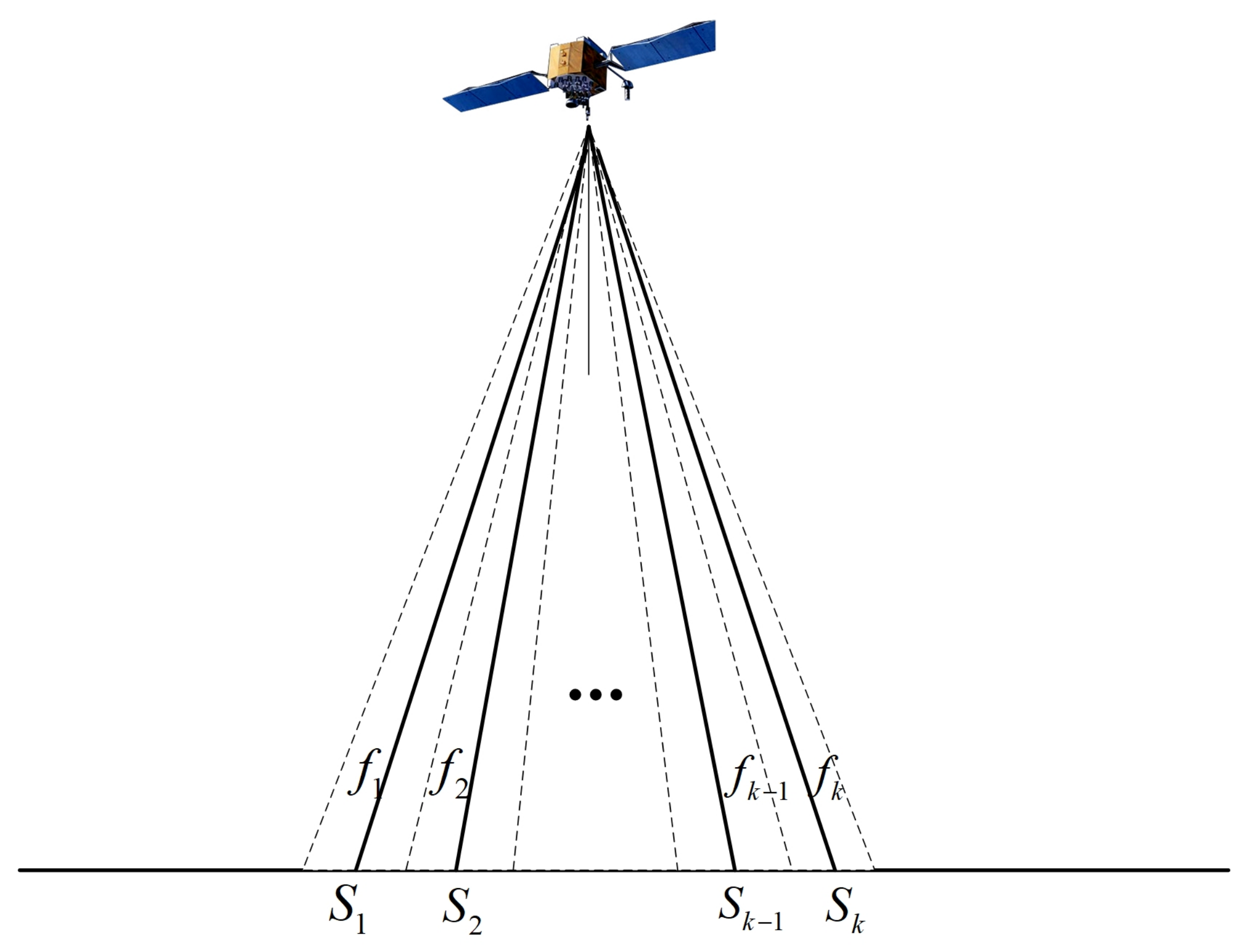
2.2.1. Sub-Aperture Processing

Generally, the beam of SAR is perpendicular to the direction of flight, and the current velocity component in the range direction is obtained by Doppler centroid estimation with full-aperture data. However, through the above analysis, in order to retrieve the current vectors, it is necessary to derive the Doppler centroids in different directions, so the data under different azimuth angles can be processed through sub-aperture processing.

In the basic theory of SAR, there is a linear relationship between Doppler frequency and azimuth time. By dividing Doppler frequency, the full-resolution image is decomposed into a series of low-resolution images formed by beams in different directions, which is sub-aperture processing technology [28].

In this method, sub-aperture data are divided in the azimuth frequency domain. The divided beam is shown in Figure 3, where the solid line represents the beam center of different sub-aperture S. The sub-aperture bandwidths are same, and the sub-aperture center frequency is $f_k$, k = 1, 2, ⋯, L, where L is the number of sub-apertures. In the ideal side-looking condition, the estimated Doppler centroid should be zero when the full-aperture beam irradiates the stationary target. However, in practical systems, the full-aperture beam is not always perpendicular to the azimuth direction. The full-aperture azimuth angle is calculated from the data recorded by the Inertial Navigation System (INS) or estimated from the data in the stationary area, such as land. According to Equation (4), the azimuth angle ${\phi }_k$ of the sub-apertures beam center line can be expressed as

$${\phi }_k=arccos\left(\frac{\lambda f_k}{2v_{p}sin\theta }\right).$$

(10)

2.2.2. Doppler Centroid Estimation

Accurate Doppler centroid estimation of real data is the basis of subsequent processing through the above analysis. According to Reference [29], the methods used for Doppler centroid estimation include the energy balance method, the power spectrum correlation method, the correlation Doppler centroid estimation method and the optimal estimation method. They use different weighting functions $B\left(f\right)$. The results of the optimal estimation method are more accurate, very close to the Cramer–Rao bound, so this paper uses this method to estimate Doppler centroid. The weighting function of optimal estimation method is shown in Equation (11), where $E\left(f\right)$ denotes the Doppler power spectrum. According to [29], Figure 4 shows $E\left(f\right)$ and $B\left(f\right)$, where $F_a$ is pulse repeat frequency (PRF). In Figure 4a, we show the Doppler bandwidth of the sub-aperture image, which corresponds to S in Figure 3. In data processing, we use a band-pass filter to extract the sub-aperture frequency band from the azimuth spectrum. The specific process is referred to in Reference [30]. The frequency point at the center of each sub-aperture bandwidth corresponds to a sub-aperture azimuth angle, and the sub-aperture azimuth angles at both ends are the extreme values, so we can get

$$B\left(f\right)=\frac{E^{\prime }\left(f\right)}{E^2\left(f\right)}.$$

(11)

As shown in Figure 4, the Doppler power spectrum $E\left(f\right)$ is an even function, while the weighting function $B\left(f\right)$ is an odd function. The convolution of the two functions has only one zero-crossing point, which is then calculated by mathematical methods such as the least squares. The zero-crossing point is the Doppler centroid frequency. We convolute the Doppler spectrum of each sub-aperture with the weighted function in Figure 4b to find the zero-crossing point, so as to estimate the Doppler centroid.

In order to accurately estimate the Doppler centroid in actual data, enough sampling points need to be taken in the azimuth and range direction for calculation. Therefore, it is necessary to block sub-aperture image data for Doppler estimation and eliminate the influence of non-geophysical terms. Finally, an average Doppler frequency for several kilometers’ range of ocean surface is acquired, which is expressed as $f_{i,j}$ ($i=1,2,\cdots ,M$, $j=1,2,\cdots ,N$, M and N represent the number of blocks in azimuth and range direction of each sub-aperture datapoint , respectively). Generally, there is a time interval between sub-aperture images, and the variation of the resulting ocean surface is usually at the pixel level. However, the Doppler estimation of sub-apertures requires thousands of pixels to obtain the mean motion state of the ocean surface over several kilometers, so it is considered that the changes of Doppler frequency between different sub-apertures are mainly caused by different beam directions, rather than the ocean surface evolution.

It should be noted that the Doppler centroid estimation process in this paper acts on the correctly imaged single look complex data for the purpose of current inversion. In some of the literature, the Doppler estimation process acts on SAR raw data to improve imaging quality, such as in [31,32]. Compared with imaging processing, this paper pays more attention to the application process of imaging data. In addition, the Doppler estimation algorithm in References [31,32] is applied to airborne SAR data with large squint and high contrast. In this paper, the squint angle of the Gaofen-3 satellite is close to zero, and the SAR data scattering is uniform and the contrast is low.

2.2.3. Vector Estimation of Ocean Current

In this section, we assume that the Doppler frequency caused by the Bragg wave phase velocity is the same at the same spatial position in each sub-aperture image. In addition, in order to improve the efficiency of the algorithm, we deal with the influence of orbital velocity through space averaging, and consider that the residual errors in the same Doppler estimation block are the same. Set the Doppler frequency shift caused by the influence of Bragg wave phase velocity and residual orbit velocity to $f_B$, and combine Equations (8) and (9), then we can get:

$$\begin{array}{cc}\hfill f_{i,j}^k& =▵f_a^k+f_c^k(i,j)+f_B(i,j)\hfill \\ \hfill & =-\frac{2}{\lambda }{v}_p▵\phi sin{\phi }_{k}sin\theta \hfill \\ \hfill & +\frac{2}{\lambda }\left(u_x\left(i,j\right)+▵\phi u_y\left(i,j\right)\right)cos{\phi }_{k}sin\theta \hfill \\ \hfill & +\frac{2}{\lambda }\left(u_y\left(i,j\right)-▵\phi u_x\left(i,j\right)\right)sin{\phi }_{k}sin\theta +f_B(i,j),\hfill \end{array}$$

(12)

where $f_{i,j}^k$ represents the Doppler results of the data block at the central coordinate $(i,j)$ of the k-th sub-aperture image. Let ${\mathbf{Y}}_{i,j}$ represent the vector composed of Doppler centroids of all L sub-aperture resolution units at spatial coordinates $(i,j)$, expressed as

$${\mathbf{Y}}_{i,j}={[f_{i,j}^1,f_{i,j}^2\cdots f_{i,j}^k\cdots f_{i,j}^L]}^T.$$

(13)

Then, the overdetermined linear equations are established and expressed in matrix form as:

$${\mathbf{Y}}_{i,j}=\mathbf{W}{\mathbf{X}}_{i,j},$$

(14)

where the coefficient matrix $\mathbf{W}$ and the unknown vector ${\mathbf{X}}_{i,j}$ containing the current information are respectively expressed as

$$\mathbf{W}=\frac{2sin\theta }{\lambda }\left[\begin{array}{cccc}-v_{p}sin{\phi }_1& cos{\phi }_1& sin{\phi }_1& \lambda /2sin\theta \\ -v_{p}sin{\phi }_2& cos{\phi }_2& sin{\phi }_2& \lambda /2sin\theta \\ ⋮& ⋮& ⋮& ⋮\\ -v_{p}sin{\phi }_L& cos{\phi }_L& sin{\phi }_L& \lambda /2sin\theta \end{array}\right]$$

(15)

$${\mathbf{X}}_{i,j}={[▵\phi ,u_x(i,j)+▵\phi u_y(i,j),u_y(i,j)-▵\phi u_x(i,j),f_B(i,j)]}^T.$$

(16)

Then, after the least squares method is used to solve ${\mathbf{X}}_{i,j}$, the azimuth velocity component $u_x$ and range velocity component $u_y$ corresponding to the data block at coordinates $(i,j)$ can be expressed as

$$u_x=\frac{X_{i,j}\left(2\right)-X_{i,j}\left(1\right)X_{i,j}\left(3\right)}{1+X_{i,j}{\left(1\right)}^2}$$

(17)

$$u_y=\frac{X_{i,j}\left(1\right)X_{i,j}\left(2\right)+X_{i,j}\left(3\right)}{1+X_{i,j}{\left(1\right)}^2}.$$

(18)

Therefore, the current velocity $u_c$ and direction ${\varphi }_c$ can be obtained:

$$u_c=\sqrt{u_x^2+u_y^2}=\sqrt{\frac{X_{i,j}^2\left(2\right)+X_{i,j}^2\left(3\right)}{1+X_{i,j}^2\left(1\right)}}.$$

(19)

$${\varphi }_c=arctan\left(\frac{u_x}{u_y}\right)=arctan\left(\frac{X_{i,j}\left(2\right)-X_{i,j}\left(1\right)X_{i,j}\left(3\right)}{X_{i,j}\left(1\right)X_{i,j}\left(2\right)+X_{i,j}\left(3\right)}\right).$$

(20)

The current field corresponding to the whole SAR image can be measured by solving the current vector of each spatial position in turn.

3. Gaofen-3 Data Experiment and Results

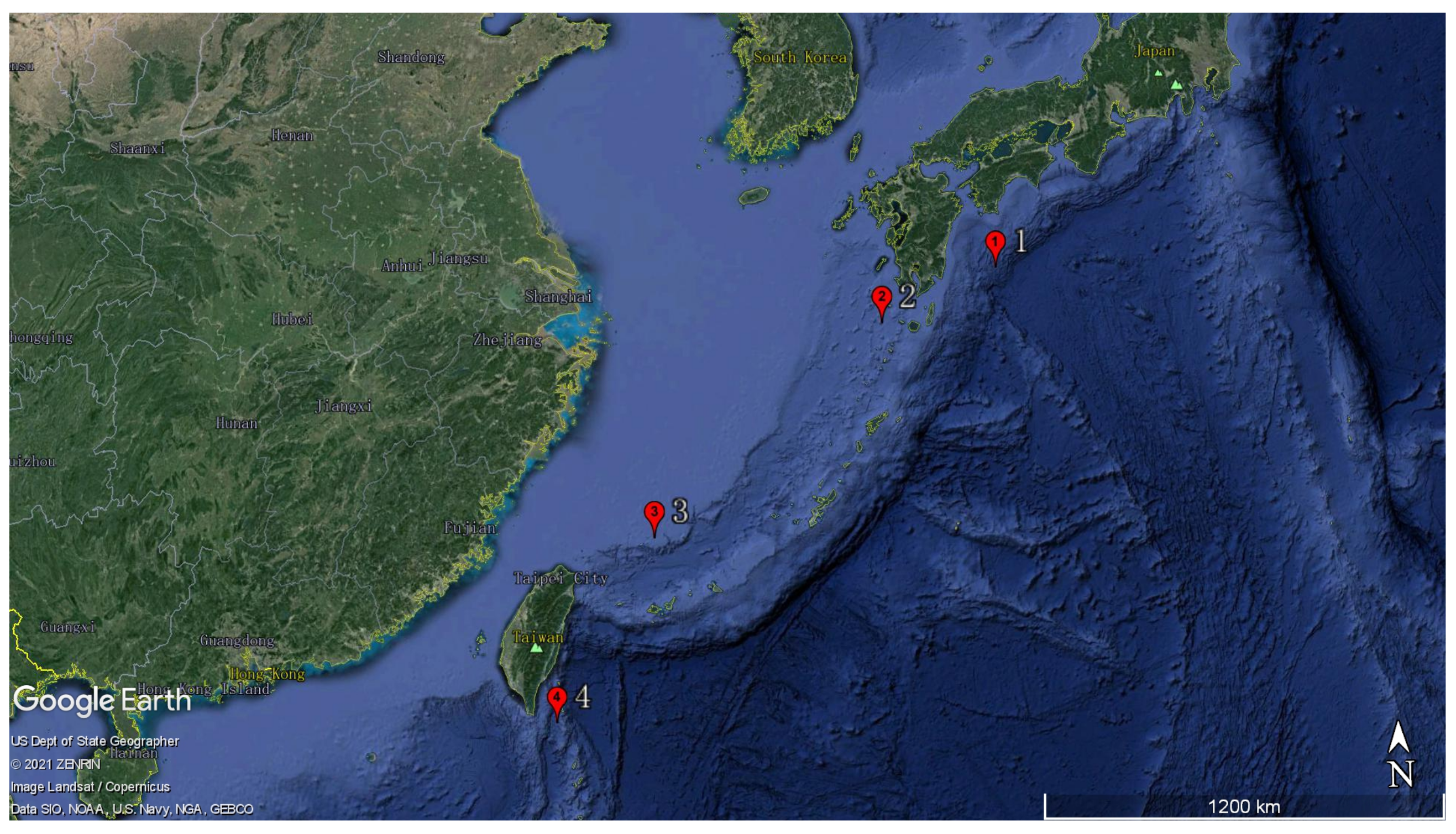
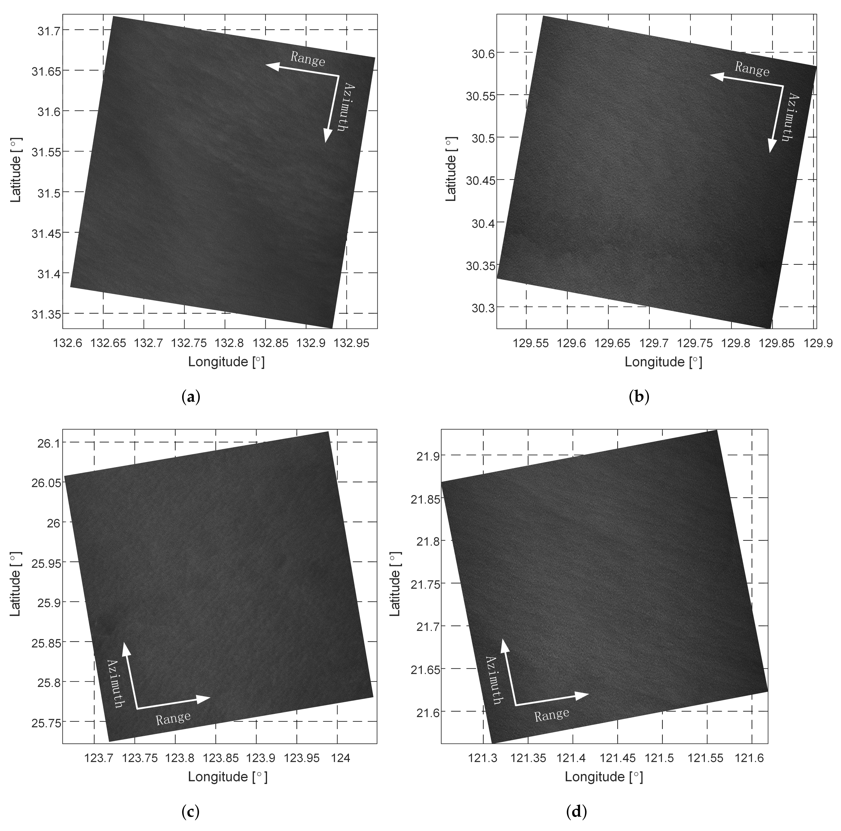
3.1. Experiment Description

The experiment site is located in the Kuroshio Current region. The Kuroshio originates from the North Equator, enters the East China Sea via the Philippines, close to the eastern part of Taiwan, and then flows through the Ryukyu Islands, along the southern part of the Japanese archipelago, and ends in the waters near 142${}^{\circ }$ E and 35${}^{\circ }$ N. The Kuroshio has the characteristics of strong flow velocity, large flow, narrow flow range, deep extension, high temperature and high salt, and so forth.

Gaofen-3 is a Chinese spacecraft carrying a C-band SAR, which was launched in August 2016, from Taiyuan (Shanxi Province, China). The Gaofen-3 satellite is capable of high resolution, large imaging width, high radiation accuracy, multiple imaging modes and long-term operation. It can monitor global marine and land information all day and all night, and expand the earth observation range and improve the rapid response capability through left–right attitude maneuver. The satellite has 12 imaging modes, which is the SAR satellite with the most imaging modes in the world. Gaofen-3 has outstanding flexibility, high attitude control accuracy and stability, and has the ability of continuous two-dimensional attitude guidance maneuver. In addition, the satellite adopts an independent health management mechanism to reduce the risk of whole satellite failure. Some Gaofen-3 SAR system parameters are shown in

Table 1. Gaofen-3 system parameters.

Parameters	Values	Units
Radar Frequency	5.4	GHz
Incidence Angle	20–60	deg
Polarization	HH/HV/VH/VV	–
Spatial Resolution	1–500	m
Swath	10–650	km
Platform Speed	7567	m/s
Orbit Altitude	755	km

. For more specific parameters and technical details, please refer to [26].

The four Gaofen-3 SAR datasets are single look complex (SLC) images acquired in ultra-fine strip-map (UFS) mode, of 3 m high resolution within 30 km swath owing to the dual-receive technique. The Gaofen-3 raw data is imaged by a special integrated SAR data processor, and a chirp scaling (CS) algorithm is used for UFS mode data. More details can be found in Reference [33]. The radar wavelength of the Gaofen-3 SAR system is 5.6 cm, the central incident angle is 22.5 degrees in ultra-fine strip-map mode. The GF-3 SAR system is right view, and implemented zero Doppler through attitude control. Further information about the data is shown in

Table 2. Gaofen-3 experimental data parameters.

Number	Date	Center Coordinates	Orbit	Polarization	Swath
1	8 May 2021	132.79${}^{\circ }$ E, 31.53${}^{\circ }$ N	Descend	HH	30 km
2	23 April 2021	129.70${}^{\circ }$ E, 30.46${}^{\circ }$ N	Descend	HH	30 km
3	15 April 2021	123.86${}^{\circ }$ E, 25.92${}^{\circ }$ N	Ascend	HH	30 km
4	16 November 2020	121.44${}^{\circ }$ E, 21.75${}^{\circ }$ N	Ascend	HH	30 km

. Figure 5 depicts the geographical locations in the red marks.

Figure 6 shows four SAR intensity images. It can be observed that all the images are relatively uniform in intensity, and are not affected by vortices, internal waves and other sea surface phenomena, which means that the weighted effect of the sea surface normalized radar cross section (NRCS) on Doppler centroid variation is minimal. Note that Johannessen et al. [6] pointed out that the Doppler estimation method works best for the quasi-uniform radar cross section, which is consistent with the image features in this experiment.

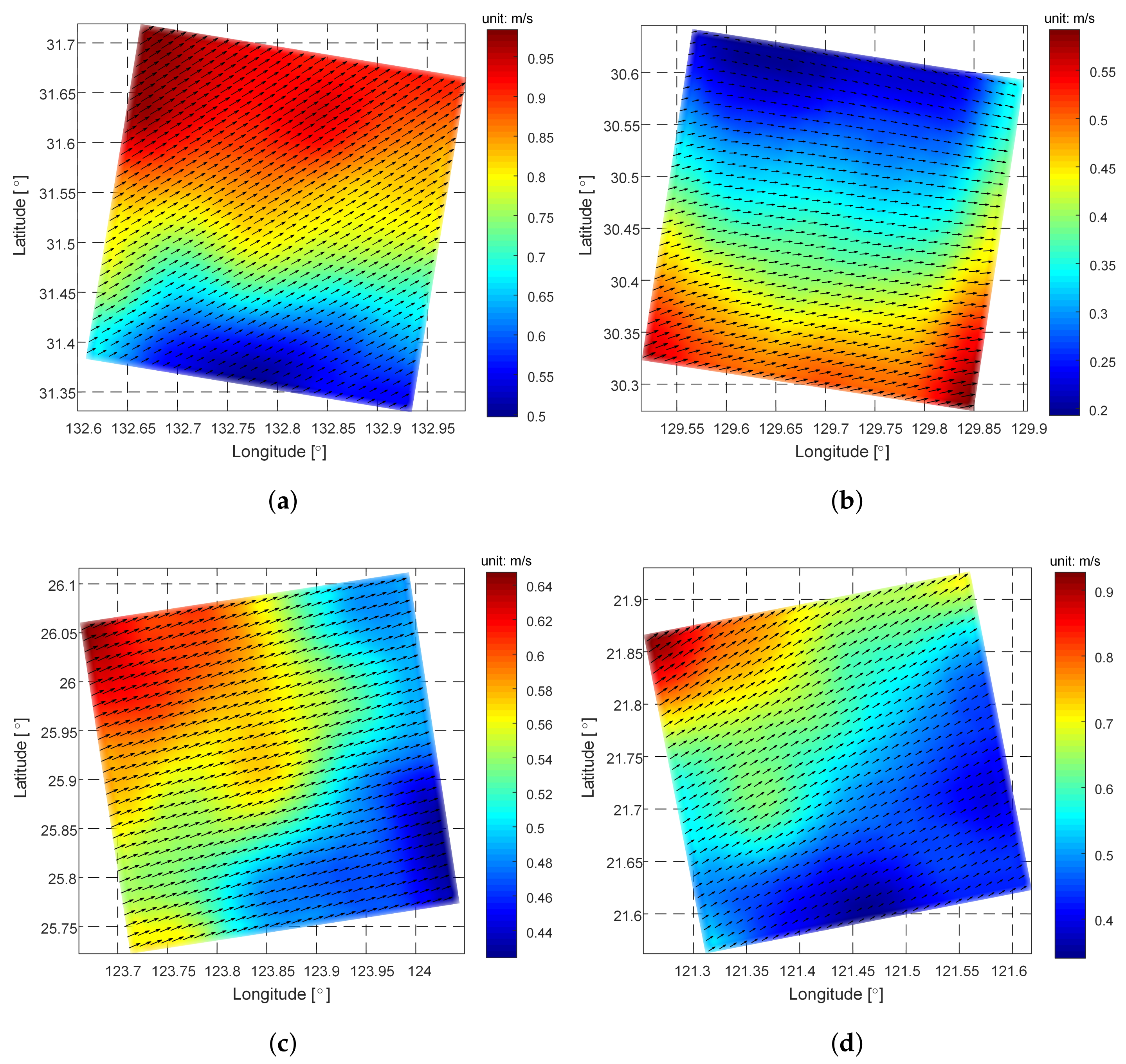
3.2. Retrieved Ocean Surface Current

In the first step of the proposed method, we extracted six sub-apertures for computation. Taking the processing result of label 1 SAR data as an example, after the first step of sub-aperture processing, one of the sub-aperture intensity images is shown in Figure 7. Obviously, the speckle noise of sub-aperture image is more serious and the resolution is reduced. In addition, the maximum azimuth angle of the sub-apertures is 0.3 degrees. In the second part, we divided each sub-aperture dataset into 30 × 30 blocks, which resulted in a grid spatial resolution of 1 km × 1 km for each block. Then, after the Doppler centroid estimation, the corresponding Doppler image is shown in Figure 7b.

In the third step, the Doppler image results of each sub-aperture data are calculated according to the flow chart, and finally the two-dimensional current field results are obtained. Corresponding to the four Gaofen-3 SAR datasets in Figure 6, the retrieved ocean surface current field after the proposed method processing is shown in Figure 8, where the color ruler and the arrow point represent the velocity and direction of the ocean current, respectively.

As can be seen from Figure 8, the ocean currents at panel (a), (c) and (d), that is, the positions at labels 1, 3 and 4 in Figure 5, are moving in a direction close to the northeast, which is consistent with the trend of the Kuroshio Current movement. Figure 8a is close to the Japanese islands, with the highest latitude, and the current velocity is the largest. In Figure 8b, the current velocity is the lowest and the direction changes, which is mainly due to the hindrance from the south of Japan island. The current field in Figure 8c is usually affected by the surrounding islands, making the velocity slower and the current direction closer to the east. Figure 8d has the lowest latitude, and the current field is closest to the equator, which is the source of the Kuroshio, so the current velocity is relatively high, and it moves northeast along the Taiwan island.

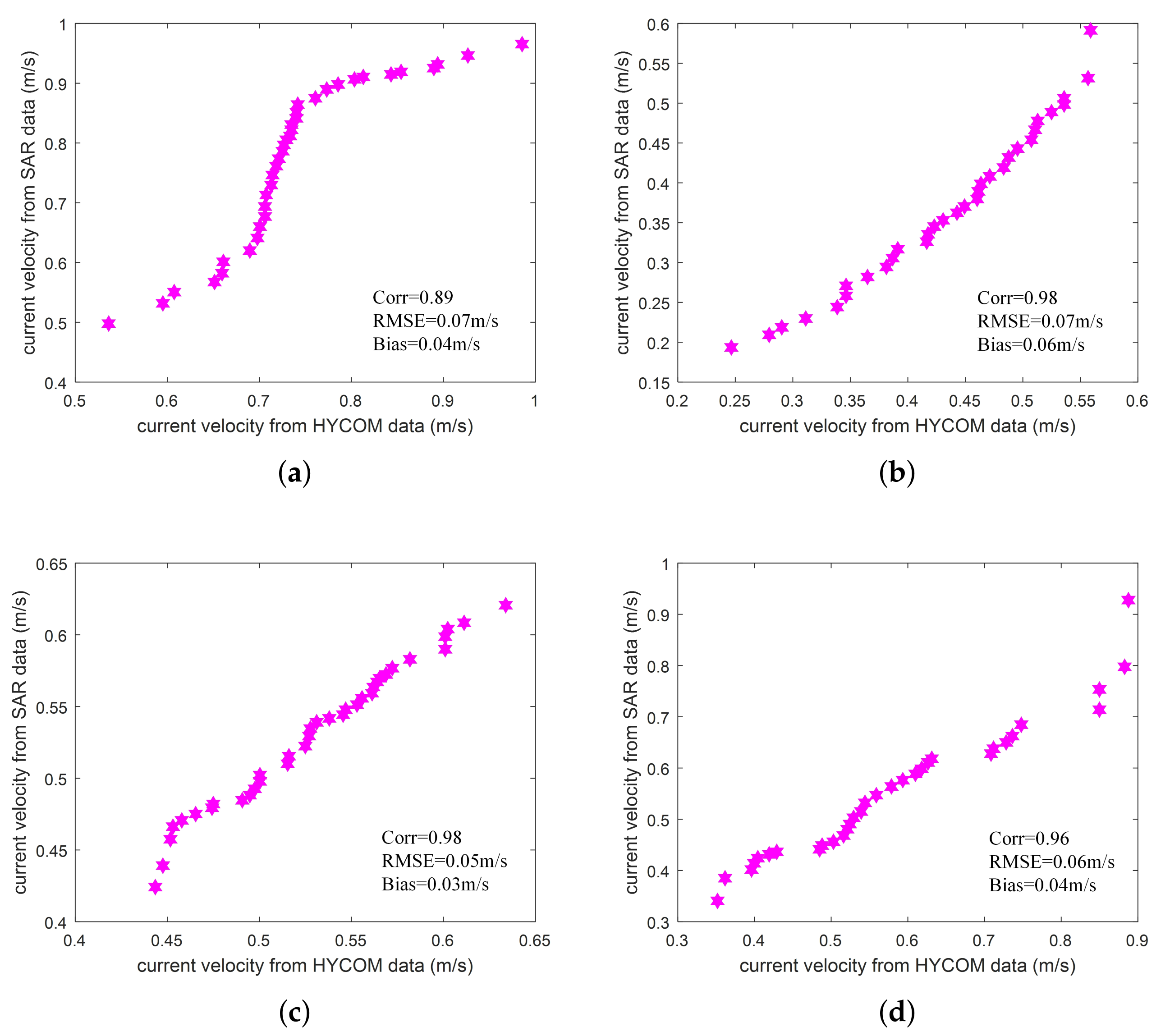
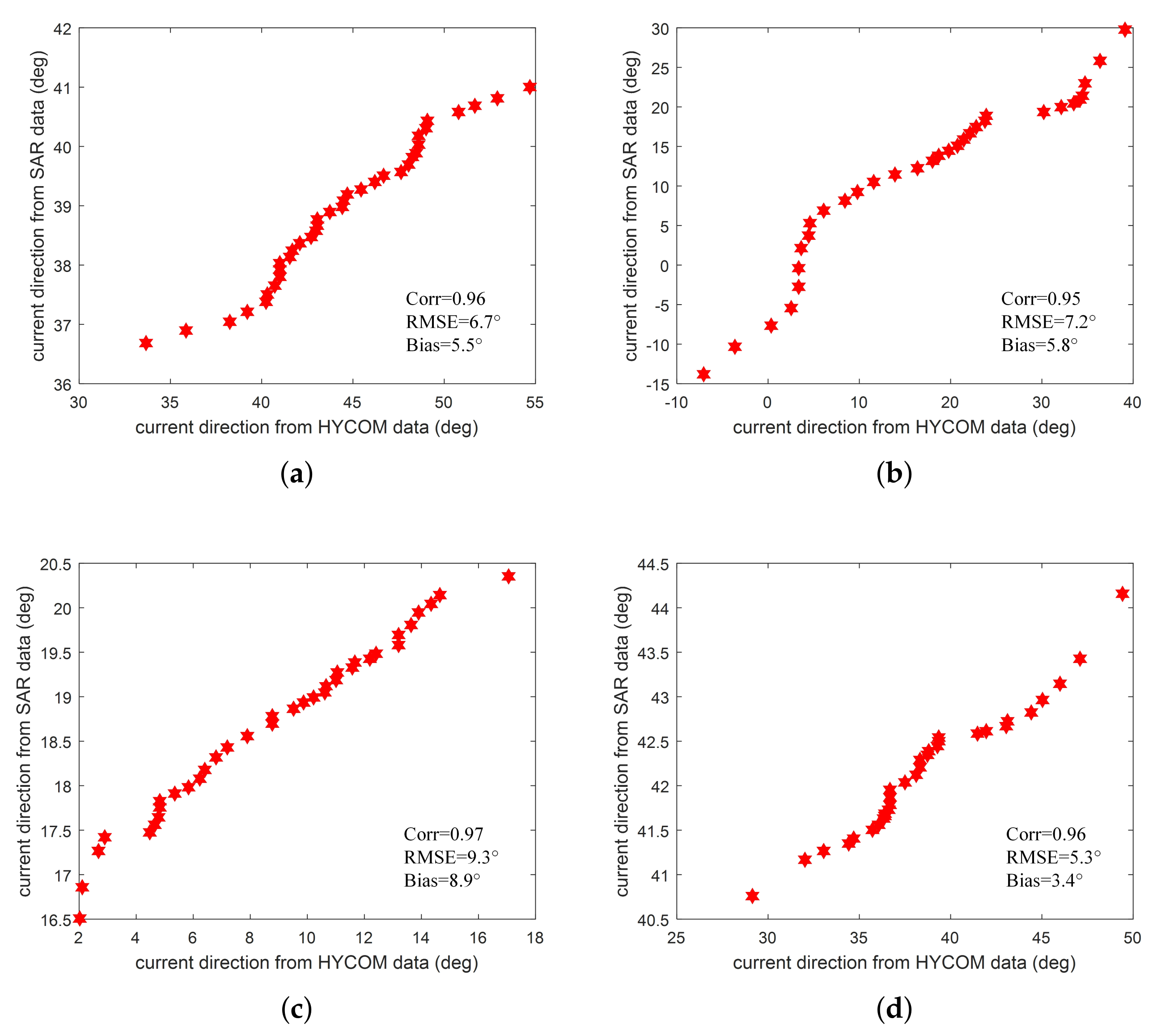
3.3. Results Validation

Generally, the in-situ data derived by Argos drifter buoys, current meters, and so forth, is optimally used for the verification of ocean current results. In addition, satellite altimeter data can also be used to verify geostrophic current. Unfortunately, there is no spatio-temporal synchronization in-situ data and altimeter data available for this experiment. In fact, since the ocean current retrieved by the altimeter is usually at a resolution of tens of kilometers, it is not suitable for comparison with the data with a smaller width and higher resolution in this article.

Ocean circulation model data can also be used for ocean current verification. The hybrid coordinate ocean model (HYCOM) has been widely used in a variety of ocean current research projects [34,35,36]. Therefore, the HYCOM model data are used to verify the results in this article. In this section, HYCOM’s global reanalysis dataset with a spatial resolution of 1/12${}^{\circ }$ and a temporal resolution of 1 day is acquired for comparison. Figure 9 shows the HYCOM ocean current model data consistent with the SAR acquisition time and location. The black box represents the boundary of the experimental area. The length and color of the arrow represent the current velocity, and the direction of the arrow indicates the current direction. It is obvious that the ocean current state in the black box compares qualitatively well with the experimental results in Figure 8.

In order to quantitatively analyze the relationship between experimental results and the model data, the results in Figure 8 were down-sampled and matched with the data in Figure 9, and the current velocity and direction scatter plots are shown in Figure 10 and Figure 11, respectively. Figure 10 illustrates the statistical comparison of current velocity, where the minimum correlation coefficient is close to 0.9 and the maximum correlation coefficient is 0.98. Both root mean square error (RMSE) and bias are less than 0.1 m/s, which meets the requirements for accuracy of current velocity measurement in marine environment applications.

Figure 11 shows the statistical comparison for the current direction results, where a direction of zero means the ocean current is going eastward. The current direction statistics of the four plots show that the correlation coefficients between the experimental results and the model data are all greater than 0.95. Both RMSE and bias are less than 10${}^{\circ }$. Although the HYCOM data represent the average state of the current field in the day, the Kuroshio current does not change much in one day. The results in Figure 10 and Figure 11 suggest that, after using the proposed method to process Gaofen-3 data, the ocean surface current fields in the Kuroshio region are measured accurately.

The current characteristics in this paper and HYCOM need to be further compared. The proposed method has the advantages of flexible data acquisition time and high spatial sampling rate. The Gaofen-3 system can image the sea area of interest and obtain the current information at specific times, with high spatial resolution of only a couple of kilometers. However, the disadvantage is that the acquisition of current field in the case of complex sea conditions and uneven sea surface scattering is not applicable, so it needs to be further studied in combination with other information. The advantage of the current field obtained from HYCOM data is that the model integrates a variety of sensor data and is applicable to a wide range of sea environment, but the disadvantage is that it only represents the average motion state of one day, and the spatial resolution is only tens of kilometers, and there is a lack of data in the nearshore sea area. Therefore, in terms of the factors that lead to the difference between the two models in retrieving the current field, the input data type and accuracy, the calculation and processing process, and the temporal and spatial characteristics of the current field products will make them different.

4. Discussion

Considering that the marine environment is complex and full of many unknowns and uncertainties, many works about ocean surface current field measurement are mainly based on data-driven studies, especially in the application of using Doppler centroids to estimate ocean currents. As mentioned in the introduction, ENVISAT ASAR data has been used to study the sea surface current field in different regions including Gulf Stream and Agulhas Stream [5,6,8]. The SAR data acquired by different systems, such as ERS [37], TerraSAR-X [38] and Sentinel-1 [39], are also used in sea surface current measurement research, respectively, demonstrating the ability of currents retrieval. The work in this paper focuses on using the Gaofen-3 SAR data to carry out application research on the ocean surface current measurement in the Kuroshio region. In terms of this, the promising experimental results have proved the current measurement capability of the Gaofen-3 system. However, it should be noted that the results will also be affected by the system, environment, and processing methods. Since there is little knowledge about the actual sea surface state, it is hard to accurately and quantitatively analyze the dynamic process of the sea surface. Nevertheless, the main influencing factors and processes of the system and environment on the experimental results will be discussed below in this section, and the applicable scope of the proposed method will be given.

The incidence angle will affect the SAR ocean surface imaging mechanism. At a medium incidence angle range from 20${}^{\circ }$ to 60${}^{\circ }$, which is consistent with the Gaofen-3 system design, the sea surface is dominated by Bragg scattering, and Bragg waves are the main scatterers on the sea surface, which is in line with the principles of the proposed method. At steep incidence angles, the specular scattering will increase imaging nonlinearity, which is not conductive to current measurement. Moreover, if the incidence angle is too large, the sea surface will be affected by wave breaking. In the experiment, the azimuth beam width determines the number of sub-apertures, which in turn also affects the current measurement results. When the azimuth beam width of the system is large, the number of sub-apertures will be more, and the number of azimuth angles will increase, which will lead to more equations used for least squares estimation to suppress the influence of random noise. However, in the case of the designed azimuth beam width, an increase in the number of sub-apertures will result in a decrease in sub-aperture time illuminating the ocean surface, which results in a decrease in the signal-to-noise ratio and current accuracy. Therefore, the number of sub-apertures is a compromise selection based on the data processing process. In this paper, six sub-apertures are used in the Gaofen-3 data experiment. Generally, in order to improve the accuracy of Doppler estimation, the size of the resolution cell for ocean current products exceeds 1 km. When the system resolution increases, the amount of data that can be used to estimate the Doppler center increases, which will also increase the accuracy of Doppler estimation. The resolution of the Gaofen-3 UFS mode data used in this paper is about 2 m, and the spatial resolution of the current field is 1 km.

Usually, the wind field will cause the variation of sea surface wave motion, resulting in the deviation of current measurement results. Therefore, in traditional current measurement methods, such as DCA and ATI, it is necessary to first estimate the deviation value using the known wind field information, and then subtract it from the current measurement results. This process makes the current measurement process more complex, and the accuracy of wind field information and the difference of deviation estimation methods will affect the current measurement accuracy. The method used in this paper does not need prior wind field information to estimate wave motion, but reasonably introduces variables representing Bragg wave phase velocity and residual orbital velocity into the equations, and finally directly solves the current information. The experimental results show that this procedure is feasible. Note that the actual sea surface environment is complex and changeable, and it is difficult to consider all the characteristics of the marine environment in one method. In this article, the experiment is located in the Kuroshio region, which has the characteristics of high current velocity and uniform ocean surface backscattering, and is less affected by strong sea surface motion phenomena such as hurricanes and vortices. These are the basic environmental features for the success of the experiment.

In summary, the method proposed in this paper is suitable for SAR systems with a medium incidence angle and high resolution, and the appropriate number of sub-apertures is selected according to the azimuth beam width and processing process. The sea surface current field with high velocity and uniform backscattering, such as Kuroshio, Agulhas current and Gulf Stream, and so forth, is an ideal measurement object. The marine environment is required to be stable without being affected by complex ocean motion phenomena.

5. Conclusions

The ocean surface current field affects global climate change and human activities, and its speed and direction information is one of the most valuable parameters in ocean research. At present, using the Doppler centroid anomaly to process a single SAR image is a commonly used method of remote sensing current measurement, and the SAR data of different systems have retrieved relatively satisfactory ocean surface radial velocities in the Gulf Stream, Agulhas Stream and other sea areas. The Kuroshio Current is also one of the largest western boundary currents in the world, but there are no more relevant experimental reports on the application of SAR data current measurement. Gaofen-3 SAR data have played an important role in retrieving ocean waves, ocean winds and other ocean parameters, but its ability to measure ocean currents needs to be verified. Therefore, this paper uses four available Gaofen-3 SAR datasets to carry out the ocean surface current measurement experiment in the Kuroshio region.

In order to derive the ocean surface current vectors, a Doppler-based current measurement method combining sub-aperture processing and the least squares technology is suggested. Instead of prior wind information, the method considers the influence of wave motion in the equations, and then estimates the current field directly. The ocean current results derived from Gaofen-3 SAR data are compared with those from ocean model data. It is found that the current velocity and direction both show good agreement. The velocity accuracy is within 0.1 m/s and the direction accuracy is within 10°, which can meet the application requirements and demonstrate the current measurement capability of Gaofen-3.

Finally, the influencing factors of the experimental process and the applicable conditions of the method are discussed. System parameters, such as incidence angle and resolution, sea conditions, and changes in the processing process, will all have an impact on the current measurement results. The proposed method is suitable for SAR data with medium incidence angle, high resolution and uniform sea surface scattering. The data processing procedures under more complex sea conditions need further research and analysis in future work.

References

1. Fischer, J.; Flemming, N.C. Operational Oceanography: Data Requirements Survey; Southampton Oceanography Centre: Southampton, UK, 1999. [Google Scholar]
2. Elyouncha, A.; Eriksson, L.E.B.; Romeiser, R.; Ulander, L.M.H. Measurements of Sea Surface Currents in the Baltic Sea Region Using Spaceborne Along-Track InSAR. IEEE Trans. Geosci. Remote Sens. 2019, 57, 8584–8599. [Google Scholar] [CrossRef]
3. Romeiser, R. The future of SAR-based oceanography: High-resolution current measurements by along-track interferometry. Oceanography 2013, 26, 92–99. [Google Scholar] [CrossRef] [Green Version]
4. Elyouncha, A.; Eriksson, L.E.B.; Romeiser, R.; Ulander, L.M.H. Empirical Relationship between the Doppler Centroid Derived from X-Band Spaceborne InSAR Data and Wind Vectors. IEEE Trans. Geosci. Remote Sens. 2021, in press. [Google Scholar] [CrossRef]
5. Chapron, B.; Collard, F.; Ardhuin, F. Direct measurements of ocean surface velocity from space: Interpretation and validation. J. Geophys. Res. Oceans 2005, 110, C07008. [Google Scholar] [CrossRef]
6. Johannessen, J.A.; Chapron, B.; Collard, F.; Kudryavtsev, V.; Mouche, A.; Akimov, D.; Dagestad, K.F. Direct ocean surface velocity measurements from space: Improved quantitative interpretation of Envisat ASAR observations. Geophys. Res. Lett. 2008, 35, L22608. [Google Scholar] [CrossRef] [Green Version]
7. Rouault, M.J.; Mouche, A.; Collard, F.; Johannessen, J.; Chapron, B. Mapping the Agulhas Current from space: An assessment of ASAR surface current velocities. J. Geophys. Res. Oceans 2010, 115, C10026. [Google Scholar] [CrossRef] [Green Version]
8. Hansen, M.W.; Collard, F.; Dagestad, K.F.; Johannessen, J.A.; Fabry, P.; Chapron, B. Retrieval of sea surface range velocities from Envisat ASAR Doppler centroid measurements. IEEE Trans. Geosci. Remote Sens. 2011, 49, 3582–3592. [Google Scholar] [CrossRef]
9. Frasier, S.J.; Carswell, J.R.; Capdevila, J. A pod-based dual-beam interferometric radar for ocean surface current vector mapping. In Proceedings of the IEEE International Geoscience and Remote Sensing Symposium (IGARSS), Sydney, NSW, Australia, 9–13 July 2004; pp. 561–563. [Google Scholar]
10. Toporkov, J.V.; Perkovic, D.; Farquharson, G.; Sletten, M.A.; Frasier, S.J. Sea surface velocity vector retrieval using dual-beam interferometry: First demonstration. IEEE Trans. Geosci. Remote Sens. 2005, 43, 2494–2502. [Google Scholar] [CrossRef]
11. Martin, A.C.H.; Gommenginger, C. Towards wide-swath high-resolution mapping of total ocean surface current vectors from space: Airborne proof-of-concept and validation. Remote Sens. Environ. 2017, 197, 58–71. [Google Scholar] [CrossRef]
12. Hwang, C.; Kao, R. TOPEX/POSEIDON-derived space–time variations of the Kuroshio Current: Applications of a gravimetric geoid and wavelet analysis. Geophys. J. Int. 2002, 151, 835–847. [Google Scholar] [CrossRef] [Green Version]
13. Chao, M.; Wu, D.; Lin, X. Variability of surface velocity in the Kuroshio Current and adjacent waters derived from Argos drifter buoys and satellite altimeter data. Chin. J. Oceanol. Limnol. 2009, 27, 208–217. [Google Scholar]
14. Yang, J.; Yuan, X.; Han, B.; Zhao, L.; Sun, J.; Shang, M.; Wang, X.; Ding, C. Phase Imbalance Analysis of GF-3 Along-Track InSAR Data and Ocean Current Measurements. Remote Sens. 2021, 13, 269. [Google Scholar] [CrossRef]
15. Yang, J.S.; Ren, L.; Wang, J. The First Quantitative Remote Sensing of Ocean Surface Waves by Chinese GF-3 SAR Satellite. Oceanol. Limnol. Sin. 2017, 48, 207–209. [Google Scholar]
16. Ren, L.; Yang, J.; Mouche, A.A.; Wang, H.; Zheng, G.; Wang, J.; Zhang, H.; Lou, X.; Chen, P. Assessments of Ocean Wind Retrieval Schemes Used for Chinese Gaofen-3 Synthetic Aperture Radar Co-Polarized Data. IEEE Trans. Geosci. Remote Sens. 2019, 57, 7075–7085. [Google Scholar] [CrossRef]
17. Yang, J.; Wang, J.; Lin, R. The first quantitative remote sensing of ocean internal waves by Chinese GF-3 SAR satellite. Acta Oceanol. Sin. 2017, 36, 118. [Google Scholar] [CrossRef]
18. Moiseev, A.; Johnsen, H.; Hansen, M.W.; Johannessen, J.A. Evaluation of Radial Ocean Surface Currents Derived From Sentinel-1 IW Doppler Shift Using Coastal Radar and Lagrangian Surface Drifter Observations. J. Geophys. Res. Oceans 2020, 125, 1–18. [Google Scholar] [CrossRef]
19. Plant, W.J. Bragg scattering of electromagnetic waves from the air/sea interface. In Surface Waves and Fluxes; Springer: Amsterdam, The Netheriands, 1990; pp. 41–108. [Google Scholar]
20. Plant, W.J.; Keller, W.C.; Hayes, K. Measurement of river surface currents with coherent microwave systems. IEEE Trans. Geosci. Remote Sens. 2005, 43, 1242–1257. [Google Scholar] [CrossRef]
21. Yurovsky, Y.Y.; Kudryavtsev, V.N.; Grodsky, S.A.; Chapron, B. Sea Surface Ka-Band Doppler Measurements: Analysis and Model Development. Remote Sens. 2019, 11, 839. [Google Scholar] [CrossRef]
22. Mouche, A.A.; Collard, F.; Chapron, B.; Dagestad, K.-F.; Guitton, G.; Johannessen, J.A.; Kerbaol, V.; Hansen, M.W. On the Use of Doppler Shift for Sea Surface Wind Retrieval From SAR. IEEE Trans. Geosci. Remote Sens. 2012, 50, 2901–2909. [Google Scholar] [CrossRef]
23. Yu, X.Z.; Chong, J.S.; Hong, W. An Iterative Method for Ocean Surface Current Retrieval by Along-track Interferometric SAR. J. Electron. Inf. Technol. 2012, 34, 2660–2665. [Google Scholar] [CrossRef]
24. Pu, W. Deep SAR Imaging and Motion Compensation. IEEE Trans. Image Process. 2021, 30, 2232–2247. [Google Scholar] [CrossRef]
25. Romeiser, R.; Schwäbisch, M.; Schulz-Stellenfleth, J. Study on Concepts for Radar Interferometry from Satellites for Ocean (and Land) Applications (KoRIOLiS); University of Hamburg: Hamburg, Germany, 2002. [Google Scholar]
26. Zhang, Q. Design and Key Technologies of the GF-3 Satellite. Acta Geod. Cartogr. Sin. 2017, 46, 269–277. [Google Scholar]
27. Pan, X.; Liao, G.; Yang, Z.; Dang, H. Sea surface current estimation using airborne circular scanning SAR with a medium grazing angle. Remote Sens. 2018, 10, 178. [Google Scholar] [CrossRef] [Green Version]
28. Ferro-Famil, L.; Reigber, A.; Pottier, E.; Boerner, W.M. Scene characterization using sub-aperture polarimetric SAR data. IEEE Trans. Geosci. Remote Sens. 2003, 41, 2264–2276. [Google Scholar] [CrossRef]
29. Bamler, R. Doppler frequency estimation and the Cramer-Rao bound. IEEE Trans. Geosci. Remote Sens. 1991, 29, 385–390. [Google Scholar] [CrossRef] [Green Version]
30. Cumming, I.; Wong, F. Digital Signal Processing of Synthetic Aperture Radar Data: Algorithms and Implementation; Artech House Incorporated: London, UK, 2005. [Google Scholar]
31. Li, W.; Huang, Y.; Yang, J.; Wu, J.; Kong, L. An Improved Radon-Transform-Based Scheme of Doppler Centroid Estimation for Bistatic Forward-Looking SAR. IEEE Geosci. Remote Sens. Lett. 2011, 8, 379–383. [Google Scholar] [CrossRef]
32. Kong, Y.; Cho, B.; Kim, Y. Ambiguity-free Doppler centroid estimation technique for airborne SAR using the Radon transform. IEEE Trans. Geosci. Remote Sens. 2005, 43, 715–721. [Google Scholar] [CrossRef]
33. Han, B.; Ding, C.; Zhong, L.; Liu, J.; Qiu, X.; Hu, Y.; Lei, B. The GF-3 SAR Data Processor. Sensors 2018, 18, 835. [Google Scholar] [CrossRef] [PubMed] [Green Version]
34. Backeberg, B.C.; Bertino, L.; Johannessen, J.A. Evaluating two numerical advection schemes in HYCOM for eddy-resolving modelling of the Agulhas Current. Ocean Sci. 2009, 5, 173–190. [Google Scholar] [CrossRef] [Green Version]
35. Seo, S.; Park, Y.-G.; Park, J.-H.; Lee, H.J.; Hirose, N.J.O.; Research, P. The Tsushima Warm Current from a high resolution ocean prediction model, HYCOM. Ocean Polar Res. 2013, 35, 135–146. [Google Scholar] [CrossRef] [Green Version]
36. Wang, M.; Liu, Z.; Zhu, X.; Yan, X.; Zhang, Z.; Zhao, R. Origin and formation of the Ryukyu Current revealed by HYCOM reanalysis. Acta Oceanol. Sin. 2019, 38, 1–10. [Google Scholar] [CrossRef]
37. Kim, J.-E.; Kim, D.-J.; Moon, W.M. Enhancement of Doppler centroid for ocean surface current retrieval from ERS-1/2 raw SAR. In Proceedings of the IEEE International Geoscience and Remote Sensing Symposium (IGARSS), Anchorage, AK, USA, 20–24 September 2004; pp. 3118–3120. [Google Scholar]
38. Rossi, C.; Runge, H.; Breit, H.; Fritz, T. Surface current retrieval from TerraSAR-X data using Doppler measurements. In Proceedings of the IEEE International Geoscience and Remote Sensing Symposium (IGARSS), Honolulu, HI, USA, 25–30 July 2010; pp. 3055–3058. [Google Scholar]
39. Johnsen, H.; Nilsen, V.; Engen, G.; Mouche, A.A.; Collard, F. Ocean doppler anomaly and ocean surface current from Sentinel 1 tops mode. In Proceedings of the IEEE International Geoscience and Remote Sensing Symposium (IGARSS), Beijing, China, 10–15 July 2016; pp. 3993–3996. [Google Scholar]
Figure 1. Schematic diagram of the geometric relationship between current and radar.
Applsci 11 07656 g001
Figure 2. Flow chart of ocean current field measurement using single antenna SAR data.
Applsci 11 07656 g002
Figure 3. Schematic diagram of sub-aperture processing.
Applsci 11 07656 g003
Figure 4. (a) Doppler power spectrum with sub-apertures bandwidth. (b) Weighting function used for Doppler centroid estimation.
Applsci 11 07656 g004
Figure 5. Geographic location of Gaofen-3 SAR data (marked in red).
Applsci 11 07656 g005
Figure 6. SAR intensity images corresponding to the four positions in Figure 5. (ad) correspond to the labels 1, 2, 3, and 4, respectively.
Applsci 11 07656 g006
Figure 7. The result of sub-aperture processing: (a) one of the sub-apertures intensity image, and the result of Doppler centroid estimation: (b) the corresponding Doppler image.
Applsci 11 07656 g007
Figure 8. The retrieved ocean surface current field corresponding to the acquisitions in Figure 6. (ad) correspond to the labels 1, 2, 3, and 4, respectively.
Applsci 11 07656 g008
Figure 9. The HYCOM model data corresponding to the ocean current results in Figure 8. (ad) correspond to the labels 1, 2, 3, and 4, respectively.
Applsci 11 07656 g009
Figure 10. The scatter plot of the current velocity after comparing the experimental results in Figure 8 with the model data in Figure 9. (ad) correspond to the labels 1, 2, 3, and 4, respectively.
Applsci 11 07656 g010
Figure 11. The scatter plot of the current direction after comparing the experimental results in Figure 8 with the model data in Figure 9. (ad) correspond to the labels 1, 2, 3, and 4, respectively.
Applsci 11 07656 g011